Frequency Response Quality Index for Assessing the Mechanical Condition of Transformer Windings

Abstract

Frequency response analysis (FRA) is a popular method for assessing a transformer’s mechanical condition. The paper proposes a new method for interpreting the frequency response measurement results. The currently used numerical indices only give one value, which may be misleading in the analysis, while the proposed frequency response quality index (FRQI) tool analyses three separate features in the whole frequency range. The applied numerical calculations technique allows for estimations of not only the values of the average quality indices, but also locally for given frequency ranges of the analysed spectrum. It allows for determination of the problems that can be found in the active part of a transformer. The presented results come from three transformers, representing cases of typical faults. Two of them are from industry, while one was used for deformational tests in laboratory conditions. The proposed FRQI method showed its usefulness in FRA test results analysis and may be introduced into the automated assessment of such data. Each of the component parameters is sensitive to other types of differences observed between the compared frequency response curves, and may be used as a good quality detection tool.

1. Introduction

Diagnostics plays a major role in power systems management. Knowledge about the actual technical condition of the devices operated by a company is the base for planning their operation, maintenance, or repairs. A very important part of the power system are the transformers, which are expensive and hard to substitute in the case of failure. Therefore, thorough diagnostics of transformers is a fast-developing branch of science and the power industry [1,2]. One of the problems that may occur in the active part of a transformer is a mechanical deformation, usually related to high-force concomitant short circuits. A loosened winding state can still be operated, but during the next event in the system, or even after there has been operations have been standard for some time, there might be a catastrophic failure. Currently, the main method used for assessing the mechanical condition of windings is frequency response analysis (FRA), which is based on the relation between the winding geometry and its frequency response (FR) over a wide frequency range [3,4]. The unresolved problem in FRA method application is still the assessment of test results. There are various methods used that are more or less automated, but usually they do not give clear results. In addition to the visual comparison of two FR curves (FRA is a comparative method) done by a human expert, various numerical indices are used, which may help in the assessment [5,6,7]. However, they usually do not have clear criteria for detecting failure and return just a single value for the analysed frequency range. This means that some dangerous changes in geometry, which give small differences between compared curves, may not be detected, while big differences in FRs, for example related to natural differences between curves (such as core magnetisation or comparison between phases), may result in an alarm value of a single numerical index. The authors propose to use a frequency response quality index (FRQI) for this purpose, because the subjective assessment of FR characteristics may lead to misleading conclusions. Also, a decision about transformer operations based on a single property of a FR curve calculated with a numerical index may be wrong. The FRQI method analyses three characteristic features of the FR. A similar approach may be found in other branches of science and technology, for example quality assessment of digital images. In this field, various quality criteria are used that define changes in the image, such as the digital signal processing algorithm (DSP). This plays an important role not only as a global parameter of quality, but also of its components, for example colour mapping, brightness level, and contrast. The research in this field is developing dynamically [8,9,10]. Such an approach inspired the authors to define the objective criteria assessing the similarities (differences) in the frequency characteristics of amplitude damping in the FRA method.

This paper introduces the FRA method, provides assumptions of the proposed method, and gives some examples of measurements assessed with the new method. The examples were chosen to cover typical failures in the active part of a transformer and the most characteristic changes in the shape of the FRA curve.

2. Frequency Response Analysis

The frequency response analysis method is based on a comparison of a sine signal applied to one end of the tested object to its response recorded at the other end. The measuring technology is already standardised [11,12], so it is possible to perform repeatable measurements. There are several test configurations, however, the standard [11] recommends using an end-to-end test connection, where the input signal is given at the beginning of the tested winding (given phase and voltage side of a transformer), the reference channel measures the signal at the same place (to remove the influence of test cables), while the second channel measures the response at the end of the winding. For Y-connected windings, the connection is A-N, B-N, C-N, while for delta connected windings it will be A-B, B-C, C-A. The remaining bushings are left open. A graphical presentation of the test circuit is given in Figure 1a. All the results provided in this paper were recorded in this test configuration. There are some important details about the measuring technology, such as a proper connection to the bushings, tap changer positions, and the correct grounding of cable screens, which should be taken into consideration, but are not the topic of this paper, so will not be discussed in detail [13,14,15].

The results of the FR measurements are presented as Bode plots, however, typically only the amplitude damping, presented in (dB), is used for the analysis. The interpretation of the obtained results is based on the comparison of two curves in the frequency range, usually from 20 Hz to 2 MHz (range recommended by a standard [11]). In a perfect case, this means that the results are compared to an earlier measurement taken in the same test configuration. In some cases, especially when the first measurement is performed on a given unit, the comparison is done between phases or on twin units, however, such results may be influenced by some additional effects [16].

The FR range can be divided into sub-bands. Typically, these are low frequency (LF), medium frequency (MF), and high frequency (HF) ranges. There is no universal division into these, as their borders depend on the geometrical size of the transformer (mainly capacitances) and some other details of construction, but some features can be used to set borders [17]. The LF range is influenced mainly by the magnetic circuit of the transformer and its bulk capacitances, forming the main parallel resonance seen for end-to-end measurement [18,19]. The MF range is sensitive to local geometry changes in the windings, therefore, it is the best area to detect deformations. This range will be used for analysis in this paper, with its borders given for each analysed case. It starts from the inflection point of the capacitive slope after the first main resonance and ends in the area where the wave phenomena starts, usually visible as a series of steep resonances related to the phase angle shifts of the next period [17]. From that point, the HF range starts, strongly influenced by local connections, test circuit parameters, and as already mentioned, wave phenomena [20,21]. An exemplary FR curve is presented in Figure 1b.

The simplest way to compare two FRA curves is visual analysis by experienced staff, but it is a subjective approach. Therefore, various methods of automated assessment are being developed, from simple mathematical formulas to artificial intelligence (AI) methods [22]. There are over a dozen numerical indices applied to such an assessment, which can be found in the literature [5,6]. However, it was found that they can be grouped into four categories, which have similar sensitivity to various failures [7]. Another problem is the lack of interpretation criteria, because numerical indices return just a single value for the analysed frequency range, which usually is the whole measured or analysed spectrum. This leads to inaccurate interpretations, as big differences between curves may be the result of differences visible in the LF range, for example, which appear quite often, despite the active part being in good condition. Other differences, visible even in the MF range, may also be misleading for analysis with a single value returned from the numerical index. This happens when the index is sensitive to a given type of difference between compared curves, for example a minimal shift of two steep parallel lines in the frequency domain (horizontal shift), which results in large difference in the vertical axis (damping). Such a shift may be forced by factors such as capacitance change related to the bushing condition or the test equipment parameters [23].

From an industrial point of view, the best approach seems to be using a good quality index that will provide information on the differences between the curves and will select cases for more complex analysis, possibly also with help of an FRA professional. Such possibilities can deliver the FRQI index, applied in this paper, which returns three values describing different sets of behaviours of FR curves.

3. Frequency Response Quality Index

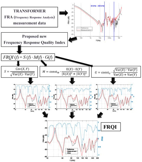
The proposed method of assessing the comparison of two datasets is based on their probabilistic properties. FRA_X (f) = {X: x_i | i = 1, 2, …, N} and FRA_y (f) = {Y: y_i | i = 1, 2, …, N} are sets of points representing two curves of FR amplitude depending on the frequency dependency from frequency f. In order to detect the differences between these two graphs, a quality index is proposed: the frequency response quality index (FRQI), which can be defined as:

FRQI (f) = S (f) ∙ M(f) ∙ G(f),

(1)

where factor S represents shapes similarity of both curves, M represents the similarity of mean values, and represents G similarity of gradients. All factors from Equation (1) are determined for a finished set of frequencies f = {f_i | i = 1, 2, …, N} contained in the range f_min ≤ f_i ≤ f_max, where f_min = f₁ and f_max = f_N. Assuming that values FRA_x and FRA_y are random variables, S, M, and G are defined:

$$S=\frac{\mathrm{Cov}\left(X,Y\right)}{\sqrt{\mathrm{Var}\left(X\right)·\mathrm{Var}\left(Y\right)}}$$

(2)

$$M={\mathrm{const}}_M·\frac{\mathrm{E}\left(X\right)·\mathrm{E}\left(Y\right)}{{\left[\mathrm{E}\left(X\right)\right]}^2+{\left[\mathrm{E}\left(Y\right)\right]}^2}$$

(3)

$$G={\mathrm{const}}_G·\frac{\sqrt{\mathrm{Var}\left(X\right)·\mathrm{Var}\left(Y\right)}}{\mathrm{Var}\left(X\right)+\mathrm{Var}\left(Y\right)}$$

(4)

where Cov(. , .) is the covariance of random variables, Var(.) is variance, E(.) is expected value, and const_M and const_G are constant values.

The algorithm for calculating the FRQI values uses estimators for the covariance, variance, and expected values. Covariances and variances are calculated with an unbiased estimation, while expected values are estimated with average values [24]. The values of the constants in Equations (3) and (4) were chosen to obtain M = 1 and G = 1 in the case of X = Y (thus FRA_X (f) = FRA_y (f)). To fulfil this condition, const_M= const_G = 2, and as a result, the values of M and G vary in the range from 0 (the worst case) to 1 (the best case). It is assumed that all values of the random variables X and Y have the same sign, namely they are only positive or only negative. This condition is usually fulfilled in FRA diagnostics if the amplitude values of separate harmonic frequencies are given in a logarithmic scale and their unit is in decibels (dB).

As already mentioned, indices M and G are the similarity measures of the mean values and gradients, respectively. The value S is—as presented in (3)—Pearson’s linear correlation coefficient [25], so its values are in the range from −1 to 1. This factor has value 1 (the best case) for linear dependency between variables X and Y, thus when y_i = ax_i + b for all i = 1, 2, …, N, where a and b are constant and a > 0. In such a case (similarity of curves’ shape FRA_X (f) and FRA_y (f)), relative similarity (differences) will be determined by M and G. Finally, the FRQI value will be from −1 to 1. For the case when a < 0 (the dependency between X and Y is still linear), the value of the coefficient S = −1. This means that the analysed curves are mirror images of one another (upside down by 180^°).

The process of the FRQI calculation, altogether with its components, is similar to the finite impulse response filter operation [26]. The data stream is subjected to successive calculations with the application of a window, which considers N = 2∙K + 1 of subsequent elements of data vector (FRA values). The window is shifted along the input vector by one element, and as a result of calculations, the vector of the output values is created. This contains 2∙K elements less than the input vector. The process of every value calculation from the values present in Equations (2)–(4) (estimate of covariance, variance, and expected value) is shown in Figure 2. The approach based on application of a sliding window of the FRA data stream was described in [27], where one of the standard numerical indices was assessed: cross-correlation factor (CCF) and its modified version.

As a result of abovementioned calculations, vectors for the values S, M, G, and FRQI are obtained. With S (f), M (f), G (f), and FRQI (f), their mean values can be easily estimated. The threshold values of FRQI and its three components, for classification of technical condition of a transformer, will depend on technical parameters of the diagnosed unit, such as power rating, construction, and vector group.

The properties of FRQI and its components can be presented in this simple example:

Two given sine functions are defined as: y₁(x) = sin(x) + 10 and y₂(x) = [A∙sin(x + β) + 10] + B, where −π ≤ x ≤ π. These two datasets (graphs) will be shifted from each other horizontally and vertically with the same amplitudes and without shifts their amplitude will also be varied. The obtained results are presented in the following graphs (Figure 3). These two sine functions, used in the following examples, are used only to present possibilities of applied indices S, M, G, and FRQI, and do not reflect the FRA datasets. The axis y represents values, while axis x is the domain of simple functions being compared.

• Case 1: A = 1, β = π/3, B = 0.

In case 1, for two curves y₁ and y₂, which differ only by a horizontal shift, significant changes can be observed in indices S (x) and G (x), while the index M (x) is almost constant. Eventually, if Equation (1) is considered, the FRQI (x) index changes its values, as shown in Figure 3e. The mean values calculated for all indices and for −π ≤ x ≤ π are: S = 0.324, M = 0.998, G = 0.666, FRQI = 0.259.

In the FRA method, such a case is the most popular. The horizontal shift of a curve (along the frequency axis) is caused by all the geometrical changes in an active part, which influence the capacitances (parallel and series). The example is an axial shift of the whole disc in the winding, resulting in the increase or decrease of the distance to neighbouring discs, and thus in capacitance changes. In some cases, inductance may also change, for example for measurements taken for various tap changer positions (a mistake during on-site measurements). Such capacitance or inductance changes influence the position of many resonances, usually visible as a horizontal shift. However, this is often accompanied by additional changes in damping or even changes in the shape of the curve (some new resonances may appear or existing ones may disappear). From Figure 3, it can be seen that such horizontal change can be detected by indices S and G. The first provides information only on local changes in the shape without taking vertical shifts into consideration, while the second returns a value for the difference between the local increments of two analysed graphs.

• Case 2: A = 1, β = 0, B = 5.

Case 2, presented in Figure 4, is a vertical shift of identical curves. As a result of calculations, no change in the values of the S and G indices was observed (S (x) = 1 and G (x) = 1). The final values for FRQI are influenced only by the M index, which can be clearly seen if curves M (x) from Figure 4b and FRQI (x) from Figure 4c are compared. For the analysed case 2, the mean values of each index for −π ≤ x ≤ π are: S = 1.000, M = 0.922, G = 1.000, FRQI = 0.922.

This case, seen in FRA curves as an amplitude change, results from resistance changes. The easiest way to achieve it is to create poor contact between the measuring clamp and the bushing, resulting in additional resistance connected in series. Any changes in resistance in the active part will also be seen as vertical changes. Damping changes usually also follow a local deformation in the windings, as already mentioned in case 1. Only the M index returns changes in the value, being a good tool for detecting amplitude changes, without any change in the shape of a FR curve.

• Case 3: A = 3, β = 0, B = 0.

In this case there are curves, which differ only by the amplitude (Figure 5). The final value of FRQI is strongly influenced by the G index, which can be clearly seen in Figure 5b,c. In case 3, the mean values of indices for −π ≤ t ≤ π are: S = 1.000, M = 0.989, G = 0.600, FRQI = 0.593.

This example is also frequently seen in FRA practice. There are many cases of damping changes in resonance points without big differences in capacitive and the inductive slopes between them. Such changes are also caused by local deformations in the windings and interference from many changes in local capacitances or mutual inductances, as many parameters from the complex structure of a transformer influence the exact position of a given resonance. In this case, the only index sensitive to such change is G, which will be a good indicator of resonance damping changes.

The presentation of the properties of the proposed method can be closed with an additional example: y₁(x) = y₂(x). In such a trivial case, the values of the indices are: S (x) = M (x) = G (x) = FRQI (x) = 1.

4. Experimental Results and Application of FRQI Index

The authors performed tests of the FRQI index on over a dozen units, finding it a useful tool for assessment. This chapter provides examples of the application of the FRQI index on measurement data obtained from three transformers, which were chosen to show various groups of differences between analysed curves. Two are units measured in industrial conditions, having visible differences between the two curves, which suggest some internal failures, while the third unit was used for deformational tests in a test substation. During such an experiment its windings were deformed and subsequent FRA measurements taken, so it has a direct correlation between the type, location, and scale of deformation and the changes in the FR curve. All measurements were taken with commercial devices available on the market in the end-to-end open test configuration, and with all requirements of the IEC 60076-18 standard fulfilled. The frequency ranges used for the analysis were set to obtain datasets connected with local geometrical changes in the transformer, so they were limited to MF only. For each case, the exact values of the analysed range are given.

4.1. Transformer No. 1

The first unit is a 160 MVA, 230/120/10.5 kV transformer, for which there was a measurement taken approximately 10 months after the reference measurement following a network event, resulting in the unit being switched off. The FRA curves can be seen in Figure 6a. The simple comparison shows a big difference in the LF range. This is an end-to-end open measurement and a clear impedance change can be seen in the low frequency region (inductive part). Such a frequency shift might suggest an incorrect tap changer position during the measurement, however the on-load tap changer (OLTC) settings were confirmed by the analysis of other tests (for different tap positions, which also show such a frequency shift). Another explanation for such a difference between the curves is a change in the core magnetisation, especially if the DC measurements were taken before the FRA tests. Such a shift is observed quite often in the industrial measurement results of FRA in the LF range and is hard to unequivocally explain. Thus, the analysis is mainly based on the MF range, which shows some differences, both in amplitude damping and in frequency shifts. This range can be seen in all following graphs from Figure 6b–e, as a background to analysis of the FRQI results. The last range, HF, shows very big differences, so there is a question about the quality of the measurement. The known history of the transformer after these measurements is as follows: the unit was allowed to be energised, then after approximately six months the FRA measurement was repeated (with other tests) and sent for internal inspection. Unfortunately, the authors do not have access to the third measurement, nor to the results of the internal inspection.

The analysis of the FRQI components follows assumptions presented in the previous point. The S index changes for values of the two datasets, where the biggest differences are present for ranges where a change of resonance direction is observed (reaching very low values at approximately 160 kHz). This index in the analysis confirms its sensitivity to such shape disturbances, which are related to serious changes in the winding geometry and are, thus, a threat to the safe operation of a transformer. The mean value for the similarity index M shows smaller differences, which follow all areas with visible changes between the datasets. It can be stated that this index is similar to the behaviour of a human expert, mostly alerted to ranges with visible differences, seen as damping changes. The gradients similarity G clearly indicates the areas where values of the two curves change in different directions (increase vs. decrease). This helps to identify ranges for very suspicious behaviour in a transformer’s FR. The last graph presents the average value of the FRQI index, with all values emphasising one another, with negative values from the S index still visible. Also, comparison of the average values of all indices for the analysed range, presented on the graphs, follows these conclusions. The lowest is index S = 0.711, while M = 0.972 and G = 0.938 are not influenced to such an extent. The total value of FRQI = 0.648, which is an indication of the existing deformation. The analysis of the FRQI shape indicates all areas where the behaviour of the two datasets is related to changes in the geometry of the test winding.

4.2. Transformer No. 2

The second transformer is a 0.4 MVA, 21/0.4 kV unit with a special purpose, used for supplying smelters. Its measurements compared between phases showed a big difference in damping, which suggested a problem with resistance in the circuit. After internal inspection, it was found that there was a problem with the internal bushing’s connection to the windings, which confirmed the diagnosis. Its LF range indicates no problems, and the differences in amplitude start with the MF range and last to the end of measured range (the end of the HF range). The full FR is presented in Figure 7a, with analysis of the FRQI components in Figure 7b–e.

The S index returns big differences (again negative values) for frequencies at which a change in the curve shape is observed. This can be a shift of resonance along the frequency axis, for example at 40 kHz, or a complete change of shape, seen in the lower part at 2 kHz. The latter case especially is related to dangerous changes in the transformer, resulting in different signal damping at this frequency (resulting from bad contact in the bushing, as was confirmed later). This is fully confirmed by the M index, which detects differences in almost the entire frequency range, from 2 kHz to 700 kHz. In this range, the value of the M index varies from approximately 0.5 to 0.8. In other words, just by observing this single index one can tell that there is a problem with additional resistance in the test circuit. The gradient similarity index G returns values similar to S, with different amplitudes for given “suspicious” ranges. The total FRQI curve strongly indicates the areas of biggest differences (the influence of S and G) and also shows the constant difference from the perfect state “1” in the whole range (due to M index). This confirms the values of all the indices, which are (from the lowest): M = 0.716, S = 0.850, and G = 0.928. The total value of FRQI = 0.565. The analysed case is quite obvious when assessed, however, it clearly presents possibilities for the proposed indices.

4.3. Transformer No. 3

The third transformer is a 0.8 MVA, 15/0.4 kV, Dyn5 distribution transformer that was used for experimental deformational tests. Its active part was lifted from the tank, some axial shifts of discs were introduced (after removing the clamping system in one phase), and it was reinserted in the tank. Thus, all measurements were taken in the original oil in the tank and the only difference was the local change in geometry. An example of a such deformation is given in Figure 8. This approach allowed for direct binding of the deformation with the change in the shape of the FR curve.

The full frequency spectrum is presented in Figure 9a. The LF range of its FR is not influenced by deformations in a significant way. In the MF range, differences start from approximately 100 kHz and result mainly in damping changes of the resonance points only. Such an effect is related to the FRQI factor changes of resonances followed by local changes of capacitances and mutual inductances, which are caused by disc shifts in the winding. The HF range is also slightly influenced in a similar way. Figure 9b–e present the analysis with the FRQI components.

In this case (deformation from Figure 8a), the S index changes its values to a much lower extent, which is expected, as the differences between two analysed curves are also much smaller than for previous transformers. The M index detects differences in the range where they appear—from approximately 200 kHz, which also is a good tendency. The third parameter G also indicates mainly the range of the biggest changes between the FR curves. The total FRQI graph is directly connected with the suspicious frequency range and allows for detection of the introduced changes. The average values of the three component indices do not change significantly (S = 0.994, M = 0.990, G = 0.996), which also influences small changes to FRQI = 0.980. Therefore, the analysis should be performed not only for the single values of all parameters, but also as their values change along the frequency (changes below 0.9 for S).

The next example is the case of a deepened axial shift by an additional disc (deformation from Figure 8b). The FR curve changes are similar to the previous example, however the differences in the resonance points are much bigger. The FR was already presented in Figure 9a, while the values of the FRQI components are given in Figure 10a–d.

The analysis of results for the second deformation leads to similar conclusions, as in the first case. Both the S and G indices are influenced strongly in this range, where the bigger differences appear between the compared FR curves, but this time they reach much lower values—down to 0.75–0.80. The M index is also more strongly influenced. The total FRQI values unequivocally indicate that there are significant differences in the FR graphs. The case of this transformer allowed for the extent of the influence of the deformation on the FRQI values to be checked. This proves that it is a sensitive tool, capable of detecting even relatively small deformations (deformation 1), dependent on the scale of the deformation (deformation 1 vs. deformation 2). The average FRQI values of three indices do not change that much (S = 0.972, M = 0.983, G = 0.987), so again—as in the case of deformation 1—there is a conclusion that it is better to analyse local changes of these indices, rather than the average value for the whole range.

5. Discussion of FRQI Results

The results presented for the three abovementioned transformers follow the assumptions of the proposed FRQI method. Each of the component indices detects different classes of differences between the two datasets. The first transformer mainly had differences between the curves seen in the damping axis, with some new resonances also appearing. All of the FRQI components were influenced, with the S index being influenced the most. This index, based on shape similarity, showed its usefulness for detecting the big differences mentioned in the curves’ shapes. The second transformer had its FR shifted in the wide frequency range, also in the vertical axis. Such a change mostly influenced the M index (similarity of the mean values), which can be a tool for detecting such wide frequency shifts. The last unit, with its two degrees of deformations introduced into the windings, influenced all component indices, as the differences between the curves were based on many features (shifts along damping) and also on the frequency scale. The last case also showed the influence of the deformation scale on the obtained results. The proposed method was proven to work properly with various types of problems in the active part, represented by specific changes in the FR characteristics.

The average value FRQI can be the first marker of suspicious changes in FRA results. It reflects the influence of all component functions S, M, and G. In the next step, if necessary, these parameters may be analysed separately.

Another important conclusion is that observation of the whole spectrum of changes will give more information on the actual condition of the transformer’s active part than only taking into account the mean values of S, M, G, and FRQI. This was confirmed by the two subsequent deformations in transformer 3. Therefore, it is suggested to use the minimum value of each index or the values change tendency rather than the mean value.

The proposed tool interprets two FRA datasets, with three separate approaches forming the final value of the FRQI. The application in numerical calculations of the moving window technique allowed for local estimation of the values of quality indices, which is very important in the case of FRA. The currently used algorithms and numerical indices, described in the literature, usually use a single value for the whole analysed frequency range (one of the exceptions is [27]). The authors, having many years of experience in the interpretation of FRA test results, find the new method very useful and its results to be more reliable than other methods. The tests were performed on almost twenty units and FRQI was shown to be employable for them all.

The average FRQI and its components S, M, and G may be easily implemented in systems of automated assessment, for example on the basis of local minimal values or the change tendency of each index. Such a tool would provide a classification of measurement results, allowing for a selection of transformers to be analysed by an experienced human expert, utilising other diagnostic tests results and the operation history.

The proposed definition of the quality index, based on the statistical properties of compared datasets, may be successfully adapted for other methods of analysis of similarities or differences between curves, such as vibroacoustic diagnostics of transformers (VM) [28], or even into other fields in science and industry.

References

- Tenbohlen, S.; Coenen, S.; Djamali, M.; Müller, A.; Samimi, M.H.; Siegel, M. Diagnostic measurements for power transformers. Energies 2016, 9, 347. [Google Scholar] [CrossRef]
- Piotrowski, T.; Rozga, P.; Kozak, R. Comparative analysis of the results of diagnostic measurements with an internal inspection of oil-filled power transformers. Energies 2019, 12, 2155. [Google Scholar] [CrossRef] [Green Version]
- Alsuhaibani, S.; Khan, Y.; Beroual, A.; Malik, N.H. A review of frequency response analysis methods for power transformer diagnostics. Energies 2016, 9, 879. [Google Scholar] [CrossRef] [Green Version]
- IEEE. IEEE Guide for the Application and Interpretation of Frequency Response Analysis for Oil-Immersed Transformers; IEEE Std C57.149-2012; IEEE: Piscataway, NJ, USA, 2013; Vol. 501, pp. 1–72. [Google Scholar]
- Samimi, M.H.; Tenbohlen, S. FRA interpretation using numerical indices: State-of-the-art. IJEPES 2017, 89, 115–125. [Google Scholar] [CrossRef]
- Samimi, M.H.; Tenbohlen, S.; Akmal, A.A.S.; Mohseni, H. Evaluation of numerical indices for the assessment of transformer frequency response. IET Gener. Transmiss. Distrib. 2016, 11, 218–227. [Google Scholar] [CrossRef]
- Banaszak, S.; Szoka, W. Transformer frequency response analysis with the grouped indices method in end-to-end and capacitive inter-winding measurement configurations. IEEE Trans. Power Deliv. 2019. (Early Access). [Google Scholar] [CrossRef]
- Wang, Z.; Bovik, A.C. A universal image quality index. IEEE Signal Process. Lett. 2002, 9, 81–84. [Google Scholar] [CrossRef]
- Seshadrinathan, K.; Soundararajan, R.; Bovik, A.; Cormack, L. Study of subjective and objective quality assessment of video. IEEE Trans. Image Proc. 2010, 19, 1427–1441. [Google Scholar] [CrossRef] [PubMed]
- Shnayderman, A.; Gusev, A.; Eskicioglu, A. An SVD-based gray-scale image quality measure for local and global assessment. IEEE Trans. Image. 2006, 15, 422–429. [Google Scholar] [CrossRef] [PubMed]
- IEC. IEC 60076-18: Power Transformers—Part 18: Measurement of Frequency Response; IEC Standard: Geneve, Switzerland, 2012. [Google Scholar]
- Miyazaki, S.; Mizutani, Y.; Tahir, M.; Tenbohlen, S. Comparison of FRA data measured by different instruments with different frequency resolution. In Proceedings of the 2018 IEEE International Conference on High Voltage Engineering and Application, Athens, Greece, 10–13 September 2018. [Google Scholar]
- Wang, M.; Vandermaar, A.J.; Srivastava, K.D. Transformer winding movement monitoring in service—Key factors affecting FRA measurements. IEEE Electr. Insul. Magaz. 2004, 20, 5–12. [Google Scholar] [CrossRef]
- Jayasinghe, J.A.S.B.; Wang, Z.D.; Jarman, P.N.; Darwin, A.W. Winding movement in power transformers: A comparison of FRA measurement connection methods. IEEE Trans. Diel. Electr. Insul. 2006, 13, 1342–1349. [Google Scholar] [CrossRef]
- Banaszak, S.; Szoka, W. Influence of a tap changer position on the transformer’s frequency response. In Proceedings of the IEEE 2018 Innovative Materials and Technologies in Electrical Engineering (i-MITEL), Sulecin, Poland, 18–20 April 2018. [Google Scholar]
- Picher, P.; Rajotte, C.; Tardif, C. Experience with frequency response analysis (FRA) for the mechanical condition assessment of transformer windings. In Proceedings of the 2013 IEEE Electrical Insulation Conference (EIC), Ottawa, Canada, 2–5 June 2013. [Google Scholar]
- Velásquez Contreras, J.L. Intelligent monitoring and diagnosis of power transformers in the context of an asset management model. Ph.D. Thesis, Polytechnic University of Catalonia (UPC), Barcelona, Spain, 2012. [Google Scholar]
- Banaszak, S. Factors influencing the position of the first resonance in the frequency response of transformer winding. Int. J. App. Electromagn. Mech. 2017, 53, 423–434. [Google Scholar]
- Gawrylczyk, K.M.; Trela, K. Frequency response modeling of transformer windings utilizing the equivalent parameters of a laminated core. Energies 2019, 12, 2371. [Google Scholar] [CrossRef] [Green Version]
- Banaszak, S.; Gawrylczyk, K.M. Wave phenomena in high-voltage windings of transformers. Acta Phys. Pol. A 2014, 125, 1335–1338. [Google Scholar] [CrossRef]
- De Gersem, H.; Henze, O.; Weiland, T.; Binder, A. Simulation of wave propagation effects in machine windings. Compel 2010, 29, 23–38. [Google Scholar] [CrossRef]
- Žarković, M.; Stojković, Z. Analysis of artificial intelligence expert systems for power transformer condition monitoring and diagnostics. Electr. Power Syst. Res. 2017, 149, 125–136. [Google Scholar] [CrossRef]
- Banaszak, S.; Gawrylczyk, K.M.; Trela, K.; Bohatyrewicz, P. The Influence of Capacitance and Inductance Changes on Frequency Response of Transformer Windings. Appl. Sci. 2019, 9, 1024. [Google Scholar] [CrossRef] [Green Version]
- Bendat, J.S.; Piersol, A.G. Random Data: Analysis and Measurement Procedures; John Wiley & Sons: Hoboken, NJ, USA, 2011. [Google Scholar]
- Bendat, J.S.; Piersol, A.G. Engineering Applications of Correlation and Spectral Analysis; John Wiley & Sons: Hoboken, NJ, USA, 1993. [Google Scholar]
- Antoniou, A. Digital Signal Processing; Mcgraw-Hill: New York, NY, USA, 2016. [Google Scholar]
- Miyazaki, S.; Mizutani, Y.; Taguchi, A.; Murakami, J.; Tsuji, N.; Takashima, M.; Kato, O. Proposal of objective criterion in diagnosis of abnormalities of power-transformer winding by Frequency Response Analysis. In Proceedings of the 2016 International Conference on Condition Monitoring and Diagnostics (CMD), Xi’an, China, 25–28 September 2016. [Google Scholar]
- Banaszak, S.; Kornatowski, E. Evaluation of FRA and VM Measurements Complementarity in the Field Conditions. IEEE Trans. Power Deliv. 2016, 31, 2123–2130. [Google Scholar] [CrossRef]
Figure 1.
(a) Test configuration of an “end-to-end open” for a Y-connected winding. (b) Example of a frequency response (FR) curve with three frequency sub-bands.
Figure 2.
The subsequent positions of a window in the process of separate estimation values in Equations (2)–(4); “+” marks the central (current) element of the window having N = 9 (K = 4) elements.
Figure 3.
The assessment results of indices S (x), M (x), G (x), and frequency response quality index (FRQI) (x) for case 1: (a) analysed curves; (b) S (x); (c) M (x); (d) G (x); (e) FRQI (x).
Figure 4.
The assessment results of indices S (x), M (x), G (x), and FRQI (x) for case 2: (a) analysed curves; (b) S (x), M (x), G (x); (c) FRQI (x).
Figure 5.
The assessment results of indices S (x), M (x), G (x), and FRQI (x) for case 3: (a) analysed curves; (b) S (x), M (x), G (x); (c) FRQI (x).
Figure 6.
The results for transformer No 1, where the analysed frequency range was from 30 kHz to 300 kHz. (a) FRA curve; (b) S index; (c) M index; (d) G index; (e) FRQI index.
Figure 7.
The results for transformer No. 2, where the analysed frequency range was from 700 Hz to 500 kHz. (a) FRA curve; (b) S index; (c) M index; (d) G index; (e) FRQI index.
Figure 8.
Deformations introduced into the winding of transformer No. 3: (a) one disc lowered for deformation 1; (b) two discs lowered for deformation 2. The rectangles on pictures point to places with removed spacers.
Figure 9.
The results of transformer No. 3 for deformation 1, where the analysed frequency ranged from 14 kHz to 700 kHz. (a) FRA curve; (b) S index; (c) M index; (d) G index; (e) FRQI index.
Figure 10.
The results of transformer No. 3 for deformation 2, where the analysed frequency ranged from 14 kHz to 700 kHz. (a) S index; (b) M index; (c) G index; (d) FRQI index.
© 2019 by the authors. Licensee MDPI, Basel, Switzerland. This article is an open access article distributed under the terms and conditions of the Creative Commons Attribution (CC BY) license (http://creativecommons.org/licenses/by/4.0/).
Share and Cite
MDPI and ACS Style
Kornatowski, E.; Banaszak, S. Frequency Response Quality Index for Assessing the Mechanical Condition of Transformer Windings. Energies 2020, 13, 29. https://0-doi-org.brum.beds.ac.uk/10.3390/en13010029
AMA Style
Kornatowski E, Banaszak S. Frequency Response Quality Index for Assessing the Mechanical Condition of Transformer Windings. Energies. 2020; 13(1):29. https://0-doi-org.brum.beds.ac.uk/10.3390/en13010029
Chicago/Turabian StyleKornatowski, Eugeniusz, and Szymon Banaszak. 2020. "Frequency Response Quality Index for Assessing the Mechanical Condition of Transformer Windings" Energies 13, no. 1: 29. https://0-doi-org.brum.beds.ac.uk/10.3390/en13010029
Note that from the first issue of 2016, this journal uses article numbers instead of page numbers. See further details here.