Comparative Study of Piezoelectric Vortex-Induced Vibration-Based Energy Harvesters with Multi-Stability Characteristics

Abstract

This work reports a comparative study on piezoelectric energy harvesting from vortex-induced vibration (VIV) with multi-stability characteristics by introducing the nonlinear magnetic forces. A lumped-parameter model for the piezoelectric cantilever-cylinder structure is considered for the sake of qualitative investigation. Firstly, the buckling displacement of harvester in monostable and bistable configurations is evaluated by virtue of a static analysis. Then, the coupled frequency and damping of the harvester varying with the electrical load resistance are determined for different values of the spacing distance between magnets. Subsequently, the dynamic behaviors and generated voltage of the harvester in two configurations are elaborately investigated, showing that varying the spacing distance is followed by a shift of lock-in region which is significant for performance optimization according to ambient wind conditions. In addition, the results show the harvester in monostable configuration displays a hardening behavior while a softening behavior takes place in bistable configuration, both of the harvester in two configurations can widen the synchronization region.

1. Introduction

The consistent development of micro-and nano-technologies associated with revolutionary advancement in wireless connectivity has resulted in innovative applications of miniature sized electronic devices including implanted [1] or wearable electronic devices [2], wireless sensing networks (WSNs) [3], mobile electronic platforms [4,5], microelectromechanical systems (MEMS) [6] and standalone wireless sensors on railway bridges which can be powered using traffic induced vibrations [7]. Although these small sensors or miniature devices need quite a low power to function, their effective large-scale application is still being hindered or restricted due to power supply issues [1,8]. The available conventional batteries have limited lifespan and require periodic replacement and cause environmental pollution, making these batteries unsuitable for future generations of standalone self-powered sensing devices [1]. Moreover, the frequent battery replacement may cause additional complications if the device is installed at an inaccessible place like a river/sea bed, bridge structures in remote areas [9], standalone high flag poles, inside the human body like in a pacemaker [10], and attached to or implanted in a wild animal in the jungle for wildlife study applications [8]. In view of this, there is an increasing demand for alternate power solutions by using energy harvesters to avoid difficulties, risks, pollutions, and cost attached with replacement of batteries [11,12]. In general, there are mainly three transduction mechanisms for energy harvesters to convert mechanical energy into electrical energy, namely, electromagnetic, piezoelectric, and electrostatic transduction. However, the piezoelectric mechanism prevails over others due to its simplicity, flexibility, and ease of application [2,6,7,10,13].

It is noted that piezoelectric energy harvesting from aeroelastic vibrations has received great attention during the past decades as it has more versatile applications in standalone sensing devices [7,9,14,15]. Particularly, a special case of flow-induced vibrations, vortex-induced vibration (VIV) was increasingly received attention owing to its unique characteristic of lock-in phenomenon where resonant oscillations of high amplitudes take place [6,12,16,17]. Mehmood et al. [6] performed computational fluid dynamics (CFD) simulations for different Reynolds numbers to explore the effects of the electrical load resistance on the oscillating amplitudes, lift coefficient, output voltage, and harvested power. Zhang et al. [18] numerically investigated VIV energy harvesting of bluff bodies with various cross-sections. Similarly, Hu et al. [19] recently carried out modeling and experimental studies of a piezoelectric energy harvester working under vortex-induced vibrations. In another important study of VIV-based energy harvesting system, Dai et al. [20] compared four different orientations of a circular cylinder working under wind flows and investigated the impacts of the orientation and flow direction on the performance of energy harvesters so that optimum orientation can be selected according to various wind conditions. Zhu et al. [21] carried out a CFD analysis of an energy harvester working under VIV and investigated the influences of a freely rotate pentagram impeller on the performance of the energy harvesting system. Alhadidi and Daqaq [15] generated a von Kármán vortex street by placing a rectangular rod in the windward direction and evaluated the voltage response as a function of the wind speed.

One of the main impediments of the designed VIV-based energy harvesters is the narrow bandwidth of the synchronization or lock-in region. This narrow bandwidth region is similar to the case of resonance phenomenon for linear energy harvesters under base excitations. To solve this issue, several research studies have been carried out in the last decade in order to design broadband energy harvesters. One of the solutions was based on including a magnetic force in the system in order to activate the multi-stability characteristics of the energy harvester. Pellegrini et al. [3] reviewed the bistable energy harvesters and concluded that the complex nonlinear dynamic response resulting in large-amplitude limit cycle is desirable for development of an efficient energy harvester. In a similar review of bistable energy harvesters, Harne et al. [22] highlighted the need for detailed investigation of effects of nonlinearities leading to bistable or multi-stable systems on power output as well as achievement of broadband synchronization region. After a critical review of using nonlinearities in the system, Daqaq et al. [1] pointed out that the performance metric normally used for linear systems cannot be extended to nonlinear systems and detailed study of nonlinear systems is required to analyze performance of nonlinear systems. The modeling and experiments of a dual cantilever piezoelectric energy harvester were carried out by Su et al. [23] who reported that a broadband synchronization region can be achieved by introducing the nonlinear magnetic force. In another study, Zhou et al. [24] utilized nonlinear magnetic force to build a doubly magnet-coupled energy harvester which can be designed in co-bistable and monostable configurations. Kim et al. [25] highlighted that bistable electromechanical oscillators have come up as a promising solution for efficient energy harvesting systems in a broadband synchronization region. Lan et al. [26] also utilized additional magnets to initiate quick switching between the wells to achieve higher output in low excitation conditions. Wang et al. [27] studied quin-stable energy harvester and proposed the use of combined nonlinearities in the system. Moreover, Jiang et al. [28] utilized multiple magnets in a snap-through orientation to develop a bistable energy harvester using buckling of the beam. Dhote et al. [29] proposed a nonlinear multimode piezoelectric vibration energy harvester with the use of geometric nonlinearity to enhance performance through magnetic interactions. Zou et al. [30] proposed to use magnetic force intervention to achieve a broadband synchronization region with higher output levels working under low excitation conditions and forced the energy harvester to vibrate within the desired area. Wang et al. [31] proposed the use of an elastic magnifier to amplify base excitations to enhance the performance of a bistable energy harvester. Masana and Daqaq [32] studied the performance of monostable and bistable energy harvesters and reported that higher accelerations are required to effectively initiate the bistable configuration in order to achieve ultra-wide synchronization regions. As for vortex-induced vibrations-based energy harvesters, an earlier study was performed by Naseer et al. [12] in which monostable characteristics of the energy harvester were deeply, studied by including the magnetic force. It was shown that hardening behavior takes place for all spacing distances with monostable characteristics. Zhang et al. [33] investigated experimentally the influences of the spacing distance between the magnets on the performance of VIV-based energy harvesters in the bistable regime. It was concluded that broadband regions with softening behaviors take place with a decrease in the harvested power compared to the conventional VIV-based energy harvester (without the magnets).

In this work, a comparative study is carried out to investigate effects of the magnetic force on the synchronization region and levels of harvested power of the energy harvester in both mono-and bi-stable regimes. To this end, a piezoelectric cantilever-cylinder structure is considered to produce energy from cross flows, owing to the occurrence of vortex-induced vibrations. Importantly, the nonlinear attractive magnetic force is utilized so that the harvester can buckle to create mono-and bi-stable configurations of harvester. With this in mind, comparisons for the output performance of harvester between monostable and bistable configurations are addressed in detail, which is not reported before. The proposed energy harvester can be switched between monostable and bistable configurations depending on the nonlinear magnetic force that can be adjusted according to the spacing distance between the magnets. Firstly, the governing equations of motion for the piezoelectric energy harvesting from vortex-induced vibrations are constructed. Then, the critical spacing distance at which buckling of the harvester occurs is determined through a static analysis. The dependence of the coupled frequency as well as damping of the energy harvester on the magnetic force is investigated. Subsequently, three pairs of spacing distances representing the energy harvester operating in monostable and bistable configurations at the same coupled frequency are selected to investigate the dynamic behaviors and output voltage of the harvester. Finally, some remarkable conclusions are drawn out.

2. Theoretical Modeling of the VIV-Based Energy Harvesting System with Multi-Stability Characteristics

The energy harvesting system under consideration consists of a cantilevered beam with a cylinder perpendicularly attached at its free end, as shown in Figure 1a. The two in-plane electrodes of unimorph piezoelectric layer adhered on each side of the beam are connected to an external electrical load resistance R. L_p represents the length of the beam covered with the piezoelectric layer while L_t denotes the total length of the beam. The thickness of piezoelectric sheet is negligible, and the electrodes are assumed to be perfectly conductive. The objective is to produce a compressive force on the beam to cause buckling behavior. Therefore, a pair of attractive magnets is introduced to result in buckling of the piezoelectric beam at a certain spacing distance (d_m) between magnets. It is noted that the induced magnetic force can be used to switch the energy harvester between monostable and bistable characteristics depending on the spacing distance [12]. Consequently, the focus of this study is to comparatively investigate the dynamics and performance of VIV-based energy harvester in monostable and bistable configurations.

For qualitative analysis, the simplified schematic for the developed lumped-parameter representation of the proposed system is depicted in Figure 1b. Then, the coupled governing equations of motion for the proposed energy harvesting system and the corresponding forces can be expressed as [12]:

$$m\ddot{x}(t)+2m\xi {\omega }_n\dot{x}(t)+m{\omega }_n{}^{2}x-\theta V+F_{mag}=F_{viv}$$

(1)

$$C_p\dot{V}+\frac{V}{R}+\theta \dot{x}=0$$

(2)

$$F_{mag}=-\frac{3x\mu a_1{a}_2}{2\pi {(x^2+d_m{}^2)}^{\frac{5}{2}}}, F_{viv}=\frac{\rho U^{2}DL}{2}.\frac{C_{L0}}{2}q-\frac{\rho UDL}{2}{C}_d\dot{x}$$

(3)

where m represents the effective mass of the energy harvesting system, x denotes the displacement of the circular cylinder, ξ is the damping ratio taken as 0.003 in the present study, C_p is the capacitance and θ represents the piezoelectric coupling coefficient.

In addition, the natural frequency is denoted by ω_n equaling to 10 Hz while the output voltage generated across the electrical load resistance is denoted by V. Note that the nonlinear magnetic force F_mag is represented in Equation (3) by using the potential energy function from dipole-dipole interaction in which µ represents the permeability constant with the value of 4$\mathsf{\pi }$10⁻⁷NA⁻², a₁ and a₂ are the effective moments of magnets, and d_m denotes the spacing distance between two magnets as depicted in Figure 1a.

Similarly, vortex-induced force F_viv is represented using the empirical representation developed by Facchinetti et al. [34], which has been validated and the results were compared with direct numerical simulations (DNS) and experiments by Violette et al. [35]. In this approach, Facchinetti et al. [35] used a modified van der Pol oscillator model to represent the fluctuating lift force in terms of circular cylinder’s acceleration by the following relationship:

$$\ddot{q}(t)+\beta {\omega }_s(q^2-1)\dot{q}+{\omega }_s{}^{2}q=\frac{A}{D}\ddot{x}$$

(4)

where ${\omega }_s$ represents the vortices’ shedding frequency with a relationship of ω_s = 2πSUD⁻¹, S is the Strouhal number taken as 0.116 in this study and U is the freestream velocity. Also, it should be noted that A and β are empirical constants with values 12 and 0.24, respectively [34]. Here, the coefficient of fluctuating lift, C_L = 0.5q(t)C_L0 can be calculated using the modified van der Pol model. In Equations (3) and (4), L is the length of the cylinder, ρ represents the density of the fluid (air in this case with value 1.225 Kg/m³), D is the diameter of proposed cylinder while C_L0 and C_d denote the steady lift and mean drag coefficients and their values in the well-developed wake region are considered to be 0.3 and 1.2, respectively.

After the incorporation of F_mag and F_viv, Equations (1), (2), and (4) represent the governing equations of the system in its reduced-order model form. In this study, the considered values for mass and diameter of the cylinder are 0.5 Kg and 0.05 m, respectively, while the length of beam is taken as 0.2 m. Furthermore, the values for electromechanical coupling θ and capacitance C_p are 1.55 × 10⁻³ and 120 × 10⁻⁹, respectively.

3. Static Analysis: Identification of Monostable and Bistable Configurations

If the spacing distance d_m is decreased, at a certain critical value denoted as d_{m_cr}, the buckling occurs, resulting in a switch of dynamic characteristics of the system from monostable configuration with one equilibrium position to bistable configuration with two stable equilibrium positions. Dropping time-dependent variables, F_viv, polarization, considering $K_m=\frac{3\mu a_1{a}_2}{2\pi }$, the static position governs the following equation of motion [12]:

$$m{\omega }_n{}^2{x}_s-\frac{3x_s{K}_m}{{(x_s{}^2+d_m{}^2)}^{\frac{5}{2}}}=0$$

(5)

The dependence of the static displacement on the spacing distance is presented in Figure 2. It can be clearly seen that there is a critical distance (d_{m_cr}) between the magnets where the equilibrium of the system is changed. When d_m > d_{m_cr}, there is a zero stable equilibrium solution ($x_s$) showing that the energy harvesting system is working in the monostable region. As d_m < d_{m_cr}, the central zero line becomes unstable resulting in a bistable configuration. The graph in Figure 2 also shows that a further decrease in the spacing distance d_m in the post-buckling scenario causes an increase in the static equilibrium displacements in a symmetric way.

4. Frequency Analysis: Multi-Stability Characteristics

Next, it is significant to evaluate the coupled frequency of the energy harvester in monostable and bistable configurations. To this end, introducing y = x − x_s as offset and substituting x into the governing equations of motion. By dropping the forcing and damping terms, the coupled frequency can be represented as [12]:

$${\omega }_c={\left({\omega }_n{}^2+\frac{1}{m}\{\frac{15K_m{x}_s{}^2}{{(x_s{}^2+d_m{}^2)}^{3.5}}-\frac{3K_m}{{(x_s{}^2+d_m{}^2)}^{2.5}}\}\right)}^{\frac{1}{2}}$$

(6)

It is noted that the modified coupled frequency depends upon the static position x_s of the system. In addition, inspecting Equation (6), we note that for the monostable scenario, when the static displacement x_s is zero, the modified frequency is directly proportional to the spacing distance d_m between magnets as shown in Figure 3.

If we keep decreasing the distance between the magnets, at critical point d_{m_cr}, the natural frequency sharply approaches to zero which indicates buckling of the system. Further decreasing the spacing distance below the critical value in the post-buckling scenario is followed by a sharp increase in the coupled frequency as clearly shown in Figure 3. Indeed, the pre-buckling scenario refers to the monostable configuration and post-buckling corresponds to the bistable configuration. In this way, the spacing distance can be adjusted as a control mechanism to switch the characteristics of the energy harvester between monostable and bistable configurations.

It should be mentioned that the considered dipole-dipole representation in our model is not valid for very small spacing distances between the magnets [36]. Therefore, in Figure 2; Figure 3, distances below 0.6 cm are not considered.

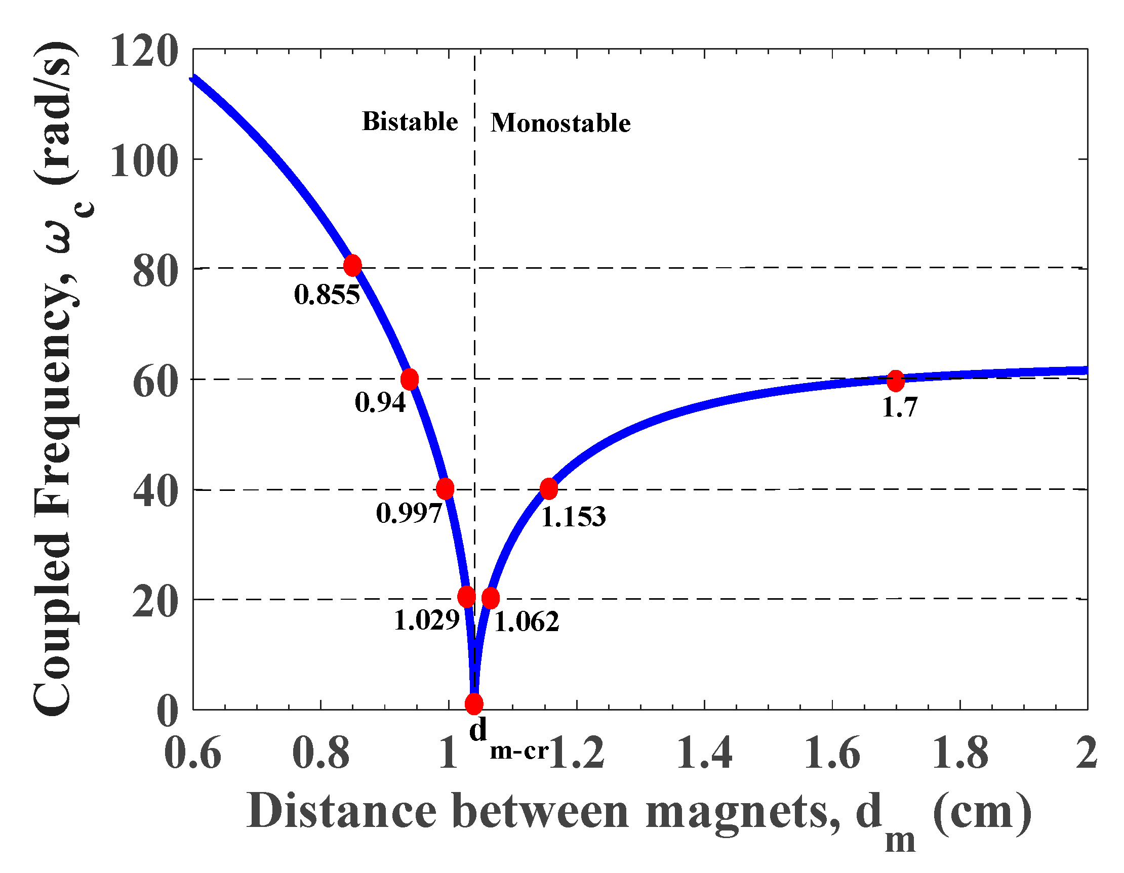
5. Selecting Key Values of d_m for Further Comparative Analysis

It should be mentioned that for further comparative analysis, four sets of spacing distances are defined as cases 1–4 as graphically shown in Figure 3 and listed in

Table 1. List of cases considered for comparative analysis.

	Coupled Frequency (rad/s)	Spacing Distance dm (cm)
		Monostable	Bistable
Case 1	20	1.062	1.029
Case 2	40	1.153	0.997
Case 3	60	1.7	0.94
Case 4	80	-	0.855

.

In order to make a better comparative analysis between monostable and bistable configurations of VIV-based energy harvesters, parameter values are selected in the way that both scenarios of the energy harvester have the same coupled frequency. For example, when the coupled frequency equals to 20 rad/s, the energy harvester can work in the monostable configuration with spacing distance of 1.062 cm while in the bistable configuration with the spacing distance of 1.029 cm. Hence, it becomes very useful to keep all other parameters constant and observe the shift from monostable configuration to bistable one as a function of the spacing distance which in turn changes the nonlinear axial force. This shift can be visible in the potential energy and phase portrait diagrams, which will be discussed later. It is noted that the monostable configuration has a maximum frequency which equals to the natural frequency of the harvester without magnetic force effect. As to the bistable configuration, the coupled frequency can increase to be much higher than the pre-buckling natural frequency of the harvester, so another point (d_m = 0.855 cm) is selected at coupled frequency of 80 rad/s to analyze the performance of the energy harvester working at a high coupled frequency. In this case, there is no corresponding monostable configuration of the energy harvester. The above-mentioned points will be consistently referred to and used in rest of the study for comparisons.

6. Linear Analysis: Effects of Load Resistance R on Coupled Frequency and Coupled Damping

In this section, we perform a linear analysis to determine the coupled frequency and damping coefficient of the energy harvester as a function of the electrical load resistance for different values of the spacing distance. In this way, the coupled equations of motion are numerically solved using the state variables. After linearization, the coupled equations of motion can be written in matrix form as:

$$\left[\begin{array}{l}{\dot{y}}_1\\ {\dot{y}}_2\\ \dot{V}\\ {\dot{q}}_1\\ {\dot{q}}_2\end{array}\right]=\left[\begin{array}{ccccc}0& 1& 0& 0& 0\\ -{\omega }_c{}^2& -2\xi {\omega }_n-\frac{F_2}{m}& \theta /m& \frac{F_1}{m}& 0\\ 0& -\theta /C_p& -1/R{C}_p& 0& 0\\ 0& 0& 0& 0& 1\\ -\alpha {\omega }_c{}^2& -2\alpha \xi {\omega }_n-\alpha F_2/m& \alpha \theta /m& -{\omega }_s{}^2+\alpha F_1/m& \beta {\omega }_s\end{array}\right]\left[\begin{array}{l}{y}_1\\ y_2\\ V\\ q_1\\ q_2\end{array}\right]$$

(7)

where:

$$\alpha =\frac{A}{D}, F_1=\frac{\rho U^{2}DL}{2}.\frac{C_L}{2}, F_2=\frac{\rho UDL}{2}{C}_d$$

The variations of the coupled frequency of the energy harvester with the electrical load resistance for different values of the spacing distance (d_m) are plotted in Figure 4a. It is noted that the selected spacing distances for the energy harvester are in either monostable or bistable configurations as depicted in Figure 3. It is found that there is a slight increase in the coupled frequency when the load resistance is between 10⁵ Ω and 10⁶ Ω for all cases of the spacing distance. Away from this region, the coupled frequency remains constant for each of spacing distance. Furthermore, one observes that the values of the coupled frequency are the same for the energy harvester in monostable and bistable scenarios for each case despite having different spacing distances which is beneficial for better performance comparison of the energy harvester between monostable and bistable configuration. Furthermore, the coupled damping of the energy harvester is plotted against the load resistance for various values of the spacing distance (d_m), as shown in Figure 4b. It is noted that there is a peak value of the coupled damping for each spacing distance and that peak lies in the range of the load resistances between 10⁵ Ω and 10⁶ Ω. Also, it should be mentioned that the peak shifts slightly to the right corresponding to the decrease of the coupled frequency.

7. Comparative Analysis: Monostable and Bistable Configurations

The dynamic behaviors and output performance of the energy harvester in monostable and bistable regimes with the same coupled frequency are investigated. Firstly, the mono-and bi-stability of each spacing distance reflected by the potential energy are recognized in Figure 5 using the following expression:

$$U=\frac{\mu a_1{a}_2}{2\pi }{(x^2+d_m{}^2)}^{-\frac{3}{2}}+\frac{1}{2}m{\omega }_n{x}^2$$

(8)

It follows from the plotted curves in Figure 5 that for spacing distances of 1.7, 1.153 and 1.062 cm, there is only one stable point locating at x = 0 cm where the potential energy is minimum. As the spacing distance is reduced to 1.029, 0.997, 0.94 and 0.855 cm, the energy harvester starts to have two stable points (centers) where the minimum potential energy occurs and one unstable point (saddle). This indicates that the energy harvesting system switches its characteristics from monostable to bistable when changing d_m.

It is reminded that the coupled frequency and damping ratio obtained above are dependent on not only the spacing distance but also the electrical load resistance, which has a significant impact on the output performance and synchronization region of the energy harvester. Consequently, in the following, the performance of the energy harvester in all four cases will be analyzed when the load resistance is 10⁵ Ω (the electromechanical damping is high), and then the load resistances of 10⁴ Ω (the electromechanical damping is low) will be considered for further comparison and analysis of the output performance.

7.1. Comparative Performance Analysis with Load Resistance of 10⁵ Ω

7.1.1. Case 1: When the Energy Harvester is Tuned to a Coupled Frequency of 20 rad/s

To compare the performance of the energy harvester for mono- and bi-stable characteristics. First, the coupled frequency is set to 20 rad/s. For the monostable configuration, the spacing distance has to be satisfied as 1.062 cm while for the bistable configuration it is 1.029 cm, as given in Table 1. Potential energies are plotted in Figure 5 which shows both monostable and bistable configurations. In Figure 5 two equilibria and a saddle in the center at x = 0 cm is visible for d_m = 1.029 cm which depicts the bistable characteristics. While for d_m = 1.062 cm, the curve shows only one equilibrium point at x = 0 cm depicting the monostable characteristics.

To make a better comparison, bifurcation diagrams for the displacement amplitudes of the energy harvester are presented when d_m = 1.062 cm for the monostable configuration given in Figure 6a while d_m = 1.029 cm for the bistable configuration offered in Figure 6b. The bifurcation diagrams clearly depict a synchronization region for each configuration. The decreasing process is used, that is to say, the wind speed is gradually decreased from the maximum value (U = 5 m/s in this case) to 1 m/s. It is important to mention that during the decreasing process, a high initial condition of x = 2 cm for the first cycle is used. After obtaining the amplitude, we use the updated displacement amplitude as the initial condition for the rest cycles. Similarly, in the increasing process, the wind speed is slowly increased from 1 m/s to 5 m/s. The initial condition for the first cycle is x = 10⁻⁶ m. Then, the updated amplitude is utilized from the previous cycle as the initial condition for the next cycle. It is found that the dynamic responses of the energy harvester in the forward and backward sweep are identical however the output levels are almost double in case of monostable configuration as compared to that in the bistable one. Also, it is noted that a softening behavior takes place in the bistable configuration while a hardening behavior takes place in the monostable configuration with negligible sharpness. This can be attributed to higher coupled electromechanical damping when selecting the load resistance of 10⁵ Ω which is able to reduce the effects of nonlinearities in both configurations with a reduction in the oscillating amplitudes and hence the levels of the harvested power.

Inspecting the bifurcation diagrams in Figure 6, the dynamical system is oscillating around the central axis in the monostable configuration. While in the bistable configuration, the system is oscillating around y = 0.15 cm. This can be expected that in the bistable configuration, the energy harvester may oscillate around one of the two stable positions at y = 0.15 cm or y = −0.15 cm or in some cases, it may oscillate around both stable axes with exhibiting the interwell oscillations which may result in higher vibration amplitudes. In order to clearly identify the dynamic response of the energy harvester in the synchronization regions, time histories and phase portraits with U = 1.6 m/s are shown in Figure 7; Figure 8, respectively. Similarly, comparison of time histories and phase portraits for wind speed U = 1.2 m/s is given in Figure 9; Figure 10, respectively. In order to compare the levels of the output power, peak values in each corresponded synchronization region are shown in Figure 11, which depicts the variations of the root mean square (RMS) output voltage as a function of the wind speed in monostable and bistable configurations.

7.1.2. Case 2: When the Harvester is Tuned to a Coupled Frequency of 40 rad/s

Next, the spacing distances between the magnets are chosen in such a way the coupled frequency is set to be 40 rad/s in both mono-and bi-stable configurations. The potential energies for both monostable and bistable configurations are plotted in Figure 5 which confirms a shift between these two configurations. The bistable configuration clearly has two lowest potential energy points corresponding to equilibrium positions and a high potential energy maximum in the middle indicating a saddle, while the monostable configuration has only one lowest energy point indicating the existence of one equilibrium position.

With consideration of the monostable and bistable configurations of harvester, in the following, bifurcation diagrams of the displacement amplitude are shown in Figure 12a,b, respectively. In the same way, the forward and backward sweep in the wind speed is utilized for a better description. Concerning the monostable configuration, it is evident from Figure 12a that decreasing and increasing processes give the same curve of dynamic responses, which may be due to the high electromechanical damping for the load resistance of R = 10⁵ Ω resulting in suppression of fluid and magnetic nonlinearities effects. As to the bistable one, however, a softening behavior for the energy harvester is visible as depicted in Figure 12b. This presents a beneficial point for broadband energy harvesting. It is also clear from Figure 12b that the energy harvesting system vibrates around different equilibrium positions with similar trends during increasing or decreasing processes. In Figure 13, time histories for both the monostable and bistable configurations are displayed and compared at U = 3.1 m/s, respectively. The plotted curves in Figure 14 are the corresponding phase portraits. These comparisons are mainly to determine which configuration is better for getting an optimum output in a certain wind speed region. Finally, Figure 15a,b show the variations of RMS generated voltage as a function of the wind speed for the monostable and bistable configurations when d_m = 1.153 cm and d_m = 0.997 cm, respectively. Clearly, a broadband synchronization region for the bistable energy harvester becomes visible. However, the output level of the voltage is lower than that for monostable configuration, especially in the peak synchronization region at the same coupled frequency, as shown in Figure 15a,b.

7.1.3. Case 3: When the Harvester is Tuned to a Coupled Frequency of 60 rad/s

In this subsection, the coupled frequency of the energy harvester is tuned to almost 60 rad/s and hence the spacing distance is adjusted to 1.7 cm for the monostable configuration and 0.94 cm for the bistable configuration. We plot in Figure 16a,b the increasing/decreasing bifurcation diagrams of the displacement amplitudes for the monostable and bistable cases, respectively. Comparing with previous cases (20 rad/s and 40 rad/s), although the dynamic responses are the same for increasing and decreasing scenarios in the monostable configuration, there is a quite clear phenomenon of softening behavior exhibiting in the bistable configuration. Obviously, the synchronization region can be clearly widened using the bistable strategy. It is clear that the energy harvesting system is vibrating around the same equilibrium position in both the increasing and decreasing scenarios and a hysteresis region occurs, which ensures a wider synchronization region in the decreasing scenario that is considered to be beneficial. To further investigate the dynamics in the synchronization region, time histories for both configurations are plotted in each of the lock-in regions, that is to say, U = 4.5 m/s for the monostable configuration and U = 3.6 m/s for the bistable configuration, as presented in Figure 17a,b. The phase curves of these time histories are also plotted in Figure 18a,b. It is noted that although the bistable configuration provides a broader synchronization region, the output level drops significantly compared to that in the monostable configuration despite the same coupled frequency of both configurations in the synchronization regions. Thus, the comparison is worth noting for further evaluation of the trends. Finally, variations of RMS generated voltage with wind speed for the monostable and bistable configurations are shown in Figure 19a,b.

A broadband synchronization region with softening behavior is evident in the bistable configuration, as depicted in Figure 19b. However, we note that the output voltage has dropped to almost half compared to that in the monostable configuration in the peak synchronization region at same coupled frequency.

7.1.4. Case 4: When the Harvester is Tuned to a Coupled Frequency of 80 rad/s

When the coupled frequency of the VIV-based energy harvesting system is adjusted to 80 rad/s, it should be mentioned that there is no corresponding monostable configuration that can be compared because this coupled frequency is beyond the maximum attainable frequency in the monostable configuration. This case of frequency is selected for further understanding the dynamics of the energy harvester operating at a very high coupled frequency and hence high wind speed environment compared to the previous cases. From the plotted curves in Figure 5, it is clear that the potential energy confirms its status as a bistable system with two stable equilibrium positions near x = 0.6 cm and x = −0.6 cm, and with x = 0 cm as an unstable equilibrium point indicating a saddle in the middle point.

The increasing/decreasing bifurcation diagrams for the displacement amplitudes are presented in Figure 20a when d_m = 0.855 cm in which the blue curve shows that decreasing the wind speed from higher initial conditions gives a significant broader synchronization region compared to that in the case of increasing scenario from low initial conditions as depicted by the red curve. A significant softening behavior takes place and it can also be noted that the energy harvester vibrates around different equilibrium positions in the case of increasing and decreasing scenarios. The plotted curves in Figure 20b show the variations of the RMS generated voltage as a function of the wind speed. The softening behavior with a hysteresis region is more prominent than the previous cases. This case is beneficial for optimizing the energy harvester in high wind speed conditions. Figure 21a,b shows, respectively, the time history and phase portrait in the hysteresis region at U = 4.4 m/s. The difference in vibration amplitude for increasing and decreasing scenarios is quite prominent.

In summary, it is demonstrated that for high coupled damping scenario as the one showed in this section, the hardening behavior for the monostable configurations is not pronounced. On the other hand, a softening behavior takes place for the bistable configurations. This softening phenomenon appears due to the presence of the quadratic nonlinearity for these bistable configurations due to the non-zero static position. Furthermore, it is shown that a decrease in the spacing distance in the bistable regime results in an increase in the nonlinear effects of the magnetic force and hence broadband synchronization regions take place when decreasing the spacing distance between the attractive magnets. It should also be mentioned that these broadband synchronization regions are not followed by an increase in the levels of the harvested power. Indeed, the monostable configurations are always better in terms of maximum levels of the harvested power.

7.2. Comparative Performance Analysis with Load Resistance of 10⁴ Ω

7.2.1. Case 1: When the Harvester is Tuned to a Coupled Frequency of 20 rad/s

Note that when the electrical load resistance is 10⁵ Ω, the energy harvester has a high coupled damping ratio which plays a key role when interacting with the nonlinearity characteristics of the system in terms of amplitudes and strength of the softening/hardening behaviors. In this part, we select R = 10⁴ Ω which gives a low coupled damping ratio to explore whether there are other nonlinear phenomena to be worth evaluating. With the same pattern in mind, Figure 22a,b shows the increasing/decreasing bifurcation diagrams of the displacement amplitude for monostable and bistable configurations, respectively. In this case, we have d_m = 1.062 cm for the monostable configuration and d_m = 1.029 cm for the bistable configuration. It is interesting that a hardening behavior can be seen in Figure 22a in monostable configuration. This hardening characteristic can be attributed to the cubic nonlinearities in the system due to the magnetic and fluid forces. Concerning the bistable configuration shown in Figure 22b, however, two broadband synchronization regions are exhibited, especially in the case of increasing the wind speed. The time histories and phase portraits for both monostable and bistable configurations are respectively plotted in Figure 23; Figure 24 at wind speed of U = 5.3 m/s. Time histories at this point show a comparable value of amplitude for both monostable and bistable configurations with periodic responses. Inspecting the bifurcation diagrams of the bistable configuration, it is clear that strange aperiodic responses take place at low wind speed values, as shown in Figure 22b. To understand this strange behavior, another set of time history and phase portrait is presented in Figure 25a,b when U = 1.2 m/s. It shows that when increasing the wind speed, the energy harvester is vibrating around two equilibrium positions as well as the two positions exhibiting intrawell oscillations. Clearly, chaotic responses take place with the presence of two attractors.

7.2.2. Case 2: When the Harvester is Tuned to a Coupled Frequency of 40 rad/s

When the coupled frequency of the VIV-based energy harvester is increased to 40 rad/s, the bifurcation diagrams for the monostable and bistable configurations are plotted in Figure 26a,b, respectively. For the case of monostable one, it shows the same trend of broadband synchronization region due to the hardening behavior. In the case of bistable scenario in Figure 26b, it is noted that two synchronization regions are visible. These results need further investigation as they may be due to the nonlinear harmonics. It should be mentioned that the limits of applicability of the Facchinetti model [35] can be violated at this level of study. However, the general trend can exist in these types of systems as shown by Masana and Daqaq [32]. Time histories for monostable and bistable configurations at wind speed of U = 5.6 m/s are plotted in Figure 27a,b, respectively. To avoid repetitive trends of graphs, the phase portraits as well as other time histories are not shown. At last, the variations of the RMS output voltage as a function of the wind speed for monostable and bistable configurations are shown in Figure 28, indicating a clear hardening behavior for monostable configuration and a softening behavior for bistable configuration. It may be noted that the nonlinearities result in secondary resonance regions in bistable scenario which may be useful in achieving broadband synchronization regions at higher wind speeds due to the presence of the quadratic nonlinearity and hence the activation of the subharmonic resonances of order 2. Moreover, it should be mentioned that the levels of the generated voltage are drastically decreased for the bistable configuration compared to the monostable one.

7.2.3. Case 3: When the Harvester is Tuned to a Coupled Frequency of 60 rad/s

When the coupled frequency is further increased to 60 rad/s, the increasing/decreasing bifurcation diagrams for the monostable and bistable configurations are plotted in Figure 29. It follows from these plots that the hardening behavior with a broadband synchronization region is clearer between wind speed of 3 m/s and 6 m/s in the case of monostable configuration. While for the bistable configuration shown Figure 29b, a softening behavior with a shift of synchronization region is obtained. The plotted curves of the RMS generated voltage for both monostable and bistable configurations are shown in Figure 30.

Clearly, the VIV-based energy harvester in monostable configuration behaves with a hardening characteristic while in bistable configuration it displays a softening characteristic and has two lock-in regions due to the quadratic nonlinearity and its importance to create the subharmonic resonance of order 2.

7.2.4. Case 4: When the Harvester Is Tuned to a Coupled Frequency of 80 rad/s

As the coupled frequency is as large as 80 rad/s, the energy harvester is only in the bistable configuration. In this case, the bifurcation diagrams for displacement amplitude are shown in Figure 31a and the RMS output voltage as a function of the wind speed is plotted in Figure 31b. Obviously, the results show a significant softening behavior and a wider hysteresis region. Inspecting the plotted curves in Figure 31a, we note that when the wind speed is around 4 m/s, the results are very interesting with quick switches of the displacement between the two equilibrium positions. To further investigate this behavior around 4 m/s, the time histories and phase portraits are plotted in Figure 32a,b, respectively. Clearly, when increasing the wind speed, intrawell oscillations take place with low amplitudes. On the other hand, when decreasing the wind speed, interwell oscillations are present and hence higher values of the displacement and generated voltage are produced.

In summary, when the electromechanical damping of the VIV-based energy harvester is low, the interaction between the magnetic and fluid nonlinearities with the linear characteristics becomes very important which significantly results in hardening and softening nonlinear behaviors for the monostable and bistable configurations, respectively. Moreover, it is proved that the presence of the quadratic nonlinearity for bistable configurations causes the appearance of important subharmonic resonances of order 2 and hence making the effectiveness of the energy harvester for an ultra-wide bandwidth of wind speeds. However, it is proved that the levels of the generated voltage and hence the harvested power are sharply decreased when considering the bistable configuration compared to its monostable counterpart. At the end, it should be stated that the considered lumped-parameter model and the modified van der Pol oscillator can be inefficient and inapplicable when low electromechanical damping ratios are considered.

8. Conclusions

In this study, a comparative analysis on the dynamic behaviors and output performance of VIV-based energy harvester has been conducted between monostable and bistable configurations which is due to the presence of nonlinear magnetic forces. The increasing and decreasing wind speed processes are performed with numerical calculations for different values of spacing distance between magnets. Two typical values of the electrical load resistance respectively associated with high and low coupled damping are considered to investigate the effect of damping on the interaction between the fluid and magnetic nonlinearities of the system. It is demonstrated that there are multiple nonlinearity factors in the system which are sensitive to various parameters like spacing distance, wind speed, load resistance, coupled frequency, and coupled damping. Consequently, the effort has been made to compare the performance of VIV-based energy harvesters in monostable and bistable regimes through a convenient parametric study. The results show that the energy harvester in the monostable configuration displays a hardening behavior with higher amplitudes and hence a larger output voltage. In the bistable configuration, the energy harvester has a wider synchronization region with period or non-period responses in the presence of subharmonic resonances of order 2, but it produces a lower output power. The output performance significantly depending on the spacing distance may provide a basis for designing an intelligent auto-tuning energy harvester. This is because we can adjust the harvester’s spacing distance to remain working within the synchronization region for maximizing the output power under various operating wind conditions.

References

1. Daqaq, M.F.; Masana, R.; Erturk, A.; Quinn, D.D. On the role of nonlinearities in vibratory energy harvesting: A critical review and discussion. Appl. Mech. Rev. 2014, 66, 040801. [Google Scholar] [CrossRef]
2. Anton, S.R.; Sodano, H.A. A review of power harvesting using piezoelectric materials (2003–2006). Smart Mater. Struct. 2007, 16, R1. [Google Scholar] [CrossRef]
3. Pellegrini, S.P.; Tolou, N.; Schenk, M.; Herder, J.L. Bistable vibration energy harvesters: A review. J. Intell. Mater. Syst. Struct. 2013, 24, 1303–1312. [Google Scholar] [CrossRef]
4. Wang, X.; Chen, C.; Wang, N.; San, H.; Yu, Y.; Halvorsen, E.; Chen, X. A frequency and bandwidth tunable piezoelectric vibration energy harvester using multiple nonlinear techniques. Appl. Energy 2017, 190, 368–375. [Google Scholar] [CrossRef]
5. Siddique, A.R.M.; Mahmud, S.; Van Heyst, B. A comprehensive review on vibration based micro power generators using electromagnetic and piezoelectric transducer mechanisms. Energy Convers. Manag. 2015, 106, 728–747. [Google Scholar] [CrossRef]
6. Mehmood, A.; Abdelkefi, A.; Hajj, M.R.; Nayfeh, A.H.; Akhtar, I.; Nuhait, A.O. Piezoelectric energy harvesting from vortex-induced vibrations of circular cylinder. J. Sound Vib. 2013, 332, 4656–4667. [Google Scholar] [CrossRef]
7. Song, Y. Finite-Element Implementation of Piezoelectric Energy Harvesting System from Vibrations of Railway Bridge. J. Energy Eng. 2018, 145, 04018076. [Google Scholar] [CrossRef]
8. Chou, S.K.; Yang, W.M.; Chua, K.J.; Li, J.; Zhang, K.L. Development of micro power generators—A review. Appl. Energy 2011, 88, 1–16. [Google Scholar] [CrossRef]
9. Yildirim, T.; Ghayesh, M.H.; Li, W.; Alici, G. A review on performance enhancement techniques for ambient vibration energy harvesters. Renew. Sustain. Energy Rev. 2017, 71, 435–449. [Google Scholar] [CrossRef] [Green Version]
10. Abdelmoula, H.; Sharpes, N.; Abdelkefi, A.; Lee, H.; Priya, S. Low-frequency Zigzag energy harvesters operating in torsion-dominant mode. Appl. Energy 2017, 204, 413–419. [Google Scholar] [CrossRef]
11. Siang, J.; Lim, M.H.; Salman Leong, M. Review of vibration-based energy harvesting technology: Mechanism and architectural approach. Int. J. Energy Res. 2018, 42, 1866–1893. [Google Scholar] [CrossRef]
12. Naseer, R.; Dai, H.; Abdelkefi, A.; Wang, L. Piezomagnetoelastic energy harvesting from vortex-induced vibrations using monostable characteristics. Appl. Energy 2017, 203, 142–153. [Google Scholar] [CrossRef]
13. Saadon, S.; Sidek, O. A review of vibration-based MEMS piezoelectric energy harvesters. Energy Convers. Manag. 2011, 52, 500–504. [Google Scholar] [CrossRef]
14. Xu, Z.; Shan, X.; Chen, D.; Xie, T. A novel tunable multi-frequency hybrid vibration energy harvester using piezoelectric and electromagnetic conversion mechanisms. Appl. Sci. 2016, 6, 10. [Google Scholar] [CrossRef] [Green Version]
15. Alhadidi, A.H.; Daqaq, M.F. A broadband bi-stable flow energy harvester based on the wake-galloping phenomenon. Appl. Phys. Lett. 2016, 109, 033904. [Google Scholar] [CrossRef] [Green Version]
16. Bernitsas, M.M.; Raghavan, K.; Simon, Y.B.; Garcia, E.M. VIVACE (Vortex Induced Vibration Aquatic Clean Energy): A new concept in generation of clean and renewable energy from fluid flow. J. Offshore Mech. Arct. Eng. 2008, 130, 041101. [Google Scholar] [CrossRef]
17. Song, R.; Shan, X.; Lv, F.; Xie, T. A study of vortex-induced energy harvesting from water using PZT piezoelectric cantilever with cylindrical extension. Ceram 2015, 41, S768–S773. [Google Scholar] [CrossRef]
18. Zhang, B.; Song, B.; Mao, Z.; Tian, W.; Li, B. Numerical investigation on VIV energy harvesting of bluff bodies with different cross sections in tandem arrangement. Energy 2017, 133, 723–736. [Google Scholar] [CrossRef]
19. Hu, Y.; Yang, B.; Chen, X.; Wang, X.; Liu, J. Modeling and experimental study of a piezoelectric energy harvester from vortex shedding-induced vibration. Energy Convers. Manag. 2018, 162, 145–158. [Google Scholar] [CrossRef]
20. Dai, H.L.; Abdelkefi, A.; Yang, Y.; Wang, L. Orientation of bluff body for designing efficient energy harvesters from vortex-induced vibrations. Appl. Phys. Lett. 2016, 108, 053902. [Google Scholar] [CrossRef]
21. Zhu, H.; Zhao, Y.; Zhou, T. CFD analysis of energy harvesting from flow induced vibration of a circular cylinder with an attached free-to-rotate pentagram impeller. Appl. Energy 2018, 212, 304–321. [Google Scholar] [CrossRef]
22. Harne, R.L.; Wang, K.W. A review of the recent research on vibration energy harvesting via bistable systems. Smart Mater. Struct. 2013, 22, 023001. [Google Scholar] [CrossRef]
23. Su, W.J.; Zu, J.; Zhu, Y. Design and development of a broadband magnet-induced dual-cantilever piezoelectric energy harvester. J. Intell. Mater. Syst. Struct. 2014, 25, 430–442. [Google Scholar] [CrossRef]
24. Zhou, S.; Cao, J.; Wang, W.; Liu, S.; Lin, J. Modeling and experimental verification of doubly nonlinear magnet-coupled piezoelectric energy harvesting from ambient vibration. Smart Mater. Struct. 2015, 24, 055008. [Google Scholar] [CrossRef]
25. Kim, P.; Nguyen, M.S.; Kwon, O.; Kim, Y.J.; Yoon, Y.J. Phase-dependent dynamic potential of magnetically coupled two-degree-of-freedom bistable energy harvester. Sci. Rep. 2016, 6, 34411. [Google Scholar] [CrossRef]
26. Lan, C.; Qin, W. Enhancing ability of harvesting energy from random vibration by decreasing the potential barrier of bistable harvester. Mech. Syst. Signal Process. 2017, 85, 71–81. [Google Scholar] [CrossRef]
27. Wang, C.; Zhang, Q.; Wang, W. Wideband quin-stable energy harvesting via combined nonlinearity. Aip Adv. 2017, 7, 045314. [Google Scholar] [CrossRef]
28. Jiang, X.Y.; Zou, H.X.; Zhang, W.M. Design and analysis of a multi-step piezoelectric energy harvester using buckled beam driven by magnetic excitation. Energy Convers. Manag. 2017, 145, 129–137. [Google Scholar] [CrossRef]
29. Dhote, S.; Yang, Z.; Behdinan, K.; Zu, J. Enhanced broadband multi-mode compliant orthoplanar spring piezoelectric vibration energy harvester using magnetic force. Int. J. Mech. Sci. 2018, 135, 63–71. [Google Scholar] [CrossRef]
30. Zou, H.X.; Zhang, W.M.; Li, W.B.; Hu, K.M.; Wei, K.X.; Peng, Z.K.; Meng, G. A broadband compressive-mode vibration energy harvester enhanced by magnetic force intervention approach. Appl. Phys. Lett. 2017, 110, 163904. [Google Scholar] [CrossRef]
31. Wang, G.; Liao, W.H.; Yang, B.; Wang, X.; Xu, W.; Li, X. Dynamic and energetic characteristics of a bistable piezoelectric vibration energy harvester with an elastic magnifier. Mech. Syst. Signal Process. 2018, 105, 427–446. [Google Scholar] [CrossRef]
32. Masana, R.; Daqaq, M.F. Relative performance of a vibratory energy harvester in mono-and bi-stable potentials. J. Sound Vib. 2011, 330, 6036–6052. [Google Scholar] [CrossRef]
33. Zhang, L.B.; Abdelkefi, A.; Dai, H.L.; Naseer, R.; Wang, L. Design and experimental analysis of broadband energy harvesting from vortex-induced vibrations. J. Sound Vib. 2017, 408, 210–219. [Google Scholar] [CrossRef]
34. Facchinetti, M.L.; de Langre, E.; Biolley, F. Coupling of structure and wake oscillators in vortex-induced vibrations. J. Fluids Struct. 2004, 19, 123–140. [Google Scholar] [CrossRef]
35. Violette, R.; Langre, E.; de Szydlowski, J. Computation of vortex-induced vibrations of long structures using a wake oscillator model: Comparison with DNS and experiments. Comput. Struct. 2007, 85, 1134–1141. [Google Scholar] [CrossRef]
36. Upadrashta, D.; Yang, Y.; Tang, L. Material strength consideration in the design optimization of nonlinear energy harvester. J. Intell. Mater. Syst. Struct. 2015, 26, 1980–1994. [Google Scholar] [CrossRef]
Figure 1. Schematics of (a) the proposed VIV-based energy harvester with top view showing direction of vibration and front view showing dimensions and (b) the equivalent spring-mass-damper representation.
Energies 13 00071 g001
Figure 2. Static position as functions of the spacing distance ‘dm’.
Energies 13 00071 g002
Figure 3. Variation of modified natural frequency as a function of the spacing distance dm between the magnets.
Energies 13 00071 g003
Figure 4. Variations of the (a) coupled frequency and (b) coupled damping ratio with load resistance R for different values of spacing distance offered in Table 1.
Energies 13 00071 g004
Figure 5. Potential energy of the harvester system for various values of dm.
Energies 13 00071 g005
Figure 6. Bifurcation diagrams of the oscillating amplitude for (a) monostable configuration at dm = 1.062 cm and (b) bistable configuration at dm = 1.029 cm.
Energies 13 00071 g006
Figure 7. Time histories at U = 1.6 m/s for (a) monostable configuration at dm = 1.062 cm and (b) bistable configuration at dm = 1.029 cm.
Energies 13 00071 g007
Figure 8. Phase portraits at U = 1.6 m/s for (a) monostable configuration at dm = 1.062 cm and (b) bistable configuration at dm = 1.029 cm.
Energies 13 00071 g008
Figure 9. Time histories at U = 1.2 m/s for (a) monostable configuration at dm = 1.062 cm and (b) bistable configuration at dm = 1.029 cm.
Energies 13 00071 g009
Figure 10. Phase portraits at U = 1.2 m/s for (a) monostable configuration at dm = 1.062 cm and (b) bistable configuration at dm = 1.029 cm.
Energies 13 00071 g010
Figure 11. Variation of output voltage as a function of wind speed for (a) monostable configuration at dm = 1.062 cm and (b) bistable configuration at dm = 1.029 cm.
Energies 13 00071 g011
Figure 12. Bifurcation diagrams of displacement amplitude for (a) monostable configuration at dm = 1.153 cm while (b) bistable configuration at dm = 0.997 cm.
Energies 13 00071 g012
Figure 13. Time histories at U = 3.1 m/s for (a) monostable configuration at dm = 1.153 cm while (b) bistable configuration at dm = 0.997 cm.
Energies 13 00071 g013
Figure 14. Phase portraits at U = 3.1 m/s for (a) monostable configuration at dm = 1.153 cm while (b) bistable configuration at dm = 0.997 cm.
Energies 13 00071 g014
Figure 15. Variation of the RMS output voltage with wind speed plotted for (a) monostable configuration at dm = 1.153 cm and (b) bistable configuration at dm = 0.997 cm.
Energies 13 00071 g015
Figure 16. Bifurcation diagrams of the displacement amplitude for (a) monostable configuration at dm = 1.7 cm and (b) bistable configuration at dm = 0.94 cm.
Energies 13 00071 g016
Figure 17. Time histories for (a) monostable configuration with dm = 1.7 cm at U = 4.5 m/s and (b) bistable configuration at dm = 0.94 cm at U = 3.6 m/s.
Energies 13 00071 g017
Figure 18. Phase portraits for (a) monostable configuration with dm = 1.7 cm at U = 4.5 m/s and (b) bistable configuration at dm = 0.94 cm at U = 3.6 m/s.
Energies 13 00071 g018
Figure 19. Variation of RMS generated voltage for (a) monostable configuration with dm = 1.7 cm and (b) bistable configuration at dm = 0.94 cm.
Energies 13 00071 g019
Figure 20. For bistable configuration at dm = 0.855 cm (a) bifurcation diagrams of displacement amplitude and (b) variation of output RMS voltage with wind speed.
Energies 13 00071 g020
Figure 21. For bistable configuration at dm = 0.855 cm, U = 4.4 m/s (a) time histories and (b) phase portrait in both increasing and decreasing scenarios.
Energies 13 00071 g021
Figure 22. For load resistance R = 104 Ohm, bifurcation diagrams of amplitude for (a) monostable configuration at dm = 1.062 cm and (b) bistable configuration at dm = 1.029 cm.
Energies 13 00071 g022
Figure 23. Time histories for at U = 5.3 m/s (a) monostable configuration with dm = 1.062 cm and (b) bistable configuration at dm = 1.029 cm.
Energies 13 00071 g023
Figure 24. Phase Portraits at U = 5.3 m/s (a) monostable configuration with dm = 1.062 cm and (b) bistable configuration at dm = 1.029 cm.
Energies 13 00071 g024
Figure 25. For bistable configuration at dm = 1.029 cm, U = 1.2 m/s (a) time histories and (b) phase portrait in both increasing and decreasing scenarios.
Energies 13 00071 g025
Figure 26. For load resistance R = 104 Ω, bifurcation diagrams of displacement amplitude for (a) monostable configuration at dm = 1.153 cm and (b) bistable configuration at dm = 0.997 cm.
Energies 13 00071 g026
Figure 27. Time histories (a) at U = 5.6 m/s for monostable configuration at dm = 1.153 cm and (b) at U = 2.5 m/s for bistable configuration at dm = 0.997 cm.
Energies 13 00071 g027
Figure 28. Variation of RMS output voltage with wind speed plotted for (a) monostable configuration at dm = 1.153 cm and (b) bistable configuration at dm = 0.997 cm.
Energies 13 00071 g028
Figure 29. For load resistance R = 104 Ohm, bifurcation diagrams of displacement amplitude for (a) monostable configuration at dm = 1.7 cm and (b) bistable configuration at dm = 0.94 cm.
Energies 13 00071 g029
Figure 30. Variation of output voltage (RMS value) with wind speed plotted for (a) monostable configuration at dm = 1.7 cm and (b) bistable configuration at dm = 0.94 cm.
Energies 13 00071 g030
Figure 31. For bistable configuration at dm = 0.855 cm (a) bifurcation diagrams of displacement amplitude and (b) variation of output voltage (RMS value) with wind speed.
Energies 13 00071 g031
Figure 32. For bistable configuration at dm = 0.855 cm, U = 4.2 m/s (a) time histories and (b) phase portrait in both increasing and decreasing scenarios.
Energies 13 00071 g032