Aquifer Thermal Energy Storage (ATES) for District Heating and Cooling: A Novel Modeling Approach Applied in a Case Study of a Finnish Urban District

Abstract

Aquifer thermal energy storage (ATES) combined with ground-source heat pumps (GSHP) offer an attractive technology to match supply and demand by efficiently recycling heating and cooling loads. This study analyses the integration of the ATES–GSHP system in both district heating and cooling networks of an urban district in southwestern Finland, in terms of technoeconomic feasibility, efficiency, and impact on the aquifer area. A novel mathematical modeling for GSHP operation and energy system management is proposed and demonstrated, using hourly data for heating and cooling demand. Hydrogeological and geographic data from different Finnish data sources is retrieved in order to calibrate and validate a groundwater model. Two different scenarios for ATES operation are investigated, limited by the maximum pumping flow rate of the groundwater area. The additional precooling exchanger in the second scenario resulted in an important advantage, since it increased the heating and cooling demand covered by ATES by 13% and 15%, respectively, and decreased the energy production cost by 5.2%. It is concluded that dispatching heating and cooling loads in a single operation, with annually balanced ATES management in terms of energy and pumping flows resulted in a low long-term environmental impact and is economically feasible (energy production cost below 30 €/MWh).

1. Introduction

According to Eurostat, in 2018, the share of renewable energy sources (RES) used for heating and cooling in EU was 21% and several countries, like Sweden (65%), Latvia (56%), Finland (55%) and Estonia (54%), covered more than half of their heating and cooling consumption with renewable sources [1]. The variability of renewable generation between heating and cooling seasons, as well as the low coincidence between supply and demand are important challenges for RES penetration, therefore short- and long-term energy storage is needed for maximizing the usage of RES. Aquifer thermal energy storage (ATES) is an attractive technological option suitable for large buildings and utilities as well as capable to enable important storage capacities [2,3]. Moreover, the utilization of GSHP operating within the urban subsurface space, is an efficient and resilient alternative for sustainable generation of heating and cooling energy in a district level [4].

The potential of ATES integration as a part of sustainable heating and cooling in combination with a ground-source heat pump (GSHP) for energy recovery from the subsurface has been acknowledged worldwide. Fleuchaus et al. [3] presented a complete overview of global ATES development and application: nowadays some 3000 ATES systems are operated worldwide. The Netherlands with 85% of all ATES realizations, followed by Sweden, Denmark and Belgium, are the undisputed frontrunners. Schmidt et al. [5] revealed that there are some 100 large-scale utility ATES systems utilized in district heating (DH) and cooling (DC) networks.

Normally, the long-term impact of ATES utilization is a combination of thermal, hydrological, microbiological and chemical impact on the affected aquifer and should be thoroughly investigated [6]. The regulation of shallow geothermal plants (depth below 400 m) varies significantly among countries [7]. Countries like Denmark, the Netherlands and Austria limit the lower and higher storage temperatures, whereas France and Switzerland establish a maximum fluctuation of groundwater temperature. Finland has no explicit legislative references to groundwater utilization for thermal storage, thus the findings of the present work can contribute for developing a specific normative framework in the future.

In the same line, the ground-source heat pump (GSHP) is a key technology for decarbonization of existing heating and cooling, which are nowadays mostly based on the use of fossil fuels [8,9,10]. The work of Paiho et al. [8] revealed the importance of large-scale heat pumps for increasing the flexibility of Finnish energy systems. Within the same research, different examples are presented for heat pump integration in Finnish DH–DC networks—including the Kakola plant in Turku utilizing heat from sewage wastewater, and the Katri Vala plant in Helsinki generating heating and cooling in a single operation.

Fleuchaus et al. [11] evaluated the performance of ATES based on different criteria and concluded that ATES integration into heating and cooling systems was rarely addressed. In order to fill this gap, the integration of GSHP in tandem with ATES within the existing DH–DC networks of a Finnish urban district is presented and developed in the current case study. The main objective of this work is to propose a mathematical modeling of the whole ATES–GSHP–DH–DC energy chain in order to improve the system’s energy management, as well as to study its technical and economic feasibility and the long-term environmental impact. Finnish public data sources are available, like the Finnish Environmental Institute (SYKE) regarding the hydrological resources, the Geological Survey of Finland (GTK) on hydrogeological conditions, and the National Land Survey of Finland (NLSF) for geographical data. The present research also introduces a methodology for fetching data from the aforementioned sources in order to calibrate and validate a groundwater model of the studied area, which in turn is an indispensable tool for studying the ATES–GSHP impact in the long-term.

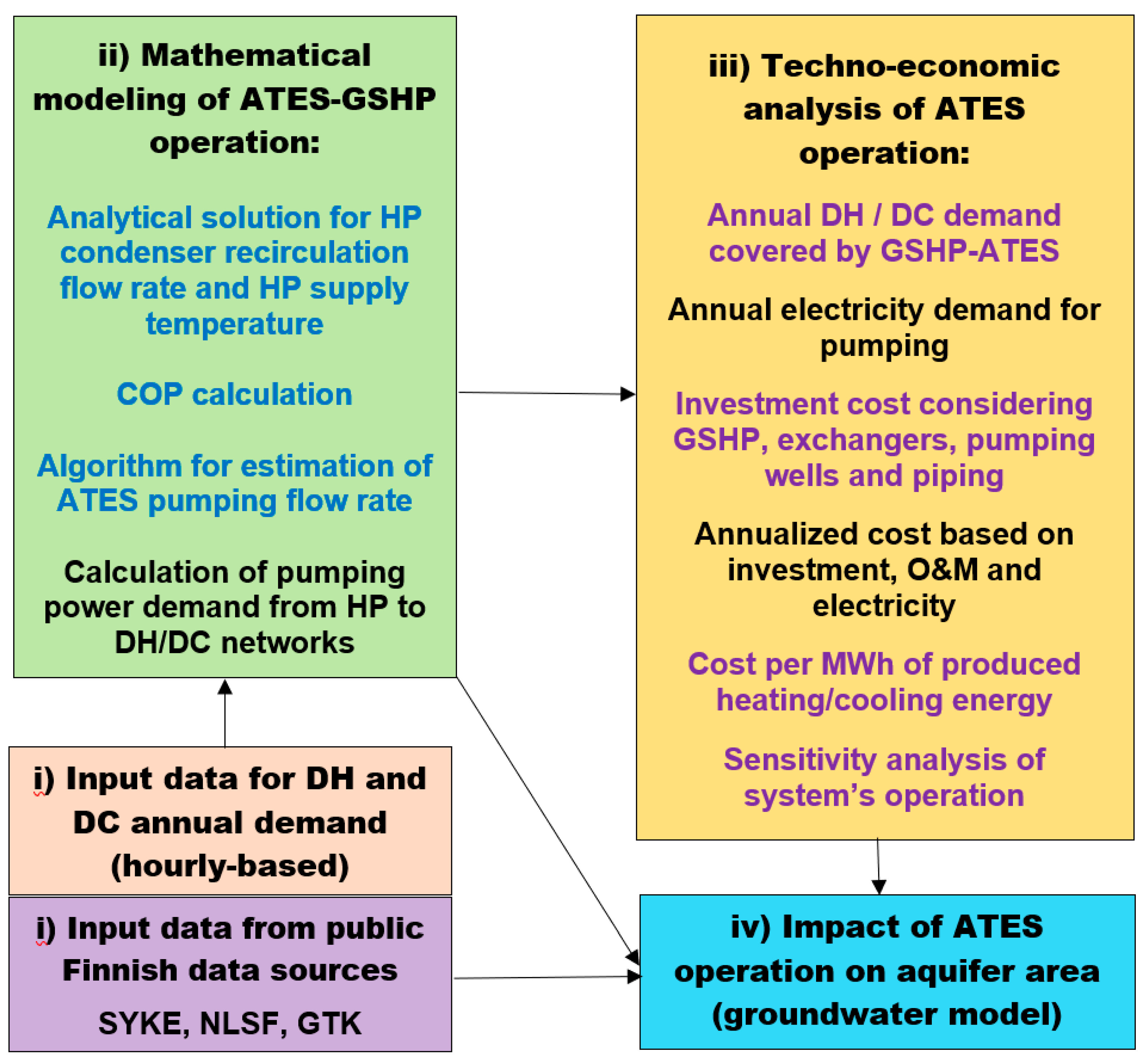
2. Materials and Methods

The modeling procedure of the combined ATES–GSHP–DH–DC system, depicted in Figure 1, is based on the following steps, namely, (i) input data of the target DH–DC networks and the nearby groundwater areas, (ii) perform mathematical modeling of combined ATES–GSHP operation, (iii) undertake technoeconomic and sensitivity analysis, and iv) study the impact of ATES operation on aquifer areas, by developing and calibrating a specific groundwater model. A groundwater model based on the finite difference method code MODFLOW (Harbaugh et al. [12]) has been adopted and developed in the present case study. The model is calibrated against long-term data (hydraulic heads of the observation wells). The particular case study is introduced in Section 2.1, while a detailed explanation and demonstration of the modeling procedure is presented in Section 2.2 and Section 2.4.

2.1. Input Data for GSHP–ATES Integration

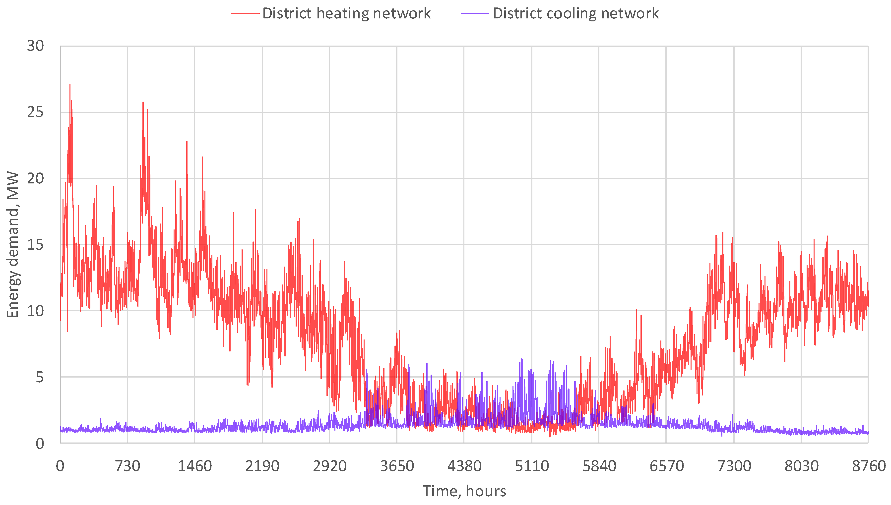
2.1.1. Input Data of the DH and DC Networks

The target district heating and cooling networks are located in the central district of Kupittaa in the town of Turku, located in the southwest part of Finland. The available data is hourly-based and the most relevant parameters of both DH and DC networks are summarized in

Table 1. Relevant DH–DC network parameters of Kupittaa district in Turku.

Relevant Network Parameters	DH Network	DC Network
Annual energy demand, MWh	67,971	12,382
Maximum/minimum load, MW	27.060/0.426	6.378/0.524
Average load (± standard deviation), MW	7.76 ± 4.8	1.41 ± 0.7
Maximum/minimum supply temperature, °C	110.4/56.0	10/5.3
Average supply temperature (± standard deviation), °C	84.3 ± 7.8	6.6 ± 0.3
Maximum/minimum return temperature, °C	51.4/22.7	14.8/10.0
Average return temperature (± standard deviation), °C	40.9 ± 2.8	13.5 ± 0.4

and Figure 2.

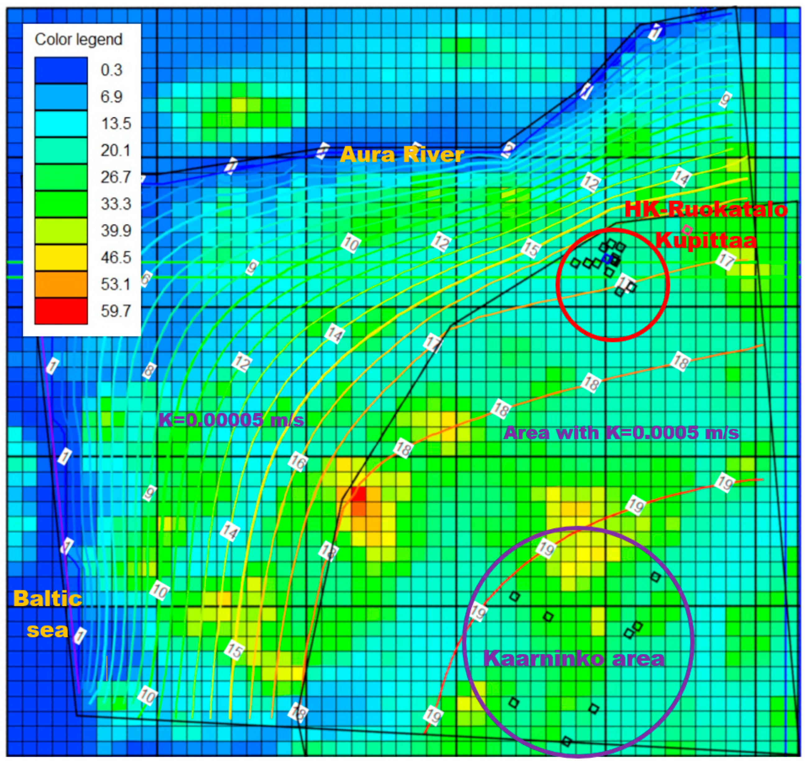
2.1.2. Input Data of the Groundwater Areas

Available open data from Finnish public sources was retrieved for characterizing the target groundwater areas. In this research, data from Finnish Environment Institute [13] was used relative to groundwater areas, monitoring stations, and observation wells. Available information was utilized for 15 observation wells located in HK-Ruokatalo area of Kupittaa district and eight wells in the Kaarninko area, and their long-term statistical data for average head were used for steady-state model calibration. In the HK-Ruokatalo area, the average measured head was 16.7 m above sea level with standard deviation 0.7 m, while for Kaarninko area these values were 19.3 m and 0.5 m respectively. The average aquifer thickness was estimated as 10 m (Joronen [14]) and the maximum allowed daily pumping rate was 2500 m³/day. The undisturbed aquifer temperature in HK-Ruokatalo area was around 10 °C, quite high due to the subsurface heat island effect observed in cities (Bayer et al. [15]).

2.1.3. Geographical Data

Open data from the National Land Survey of Finland [16] was used, particularly its “10 m elevation model”. The elevation model was retrieved as Geo-TIFF raster file and transformed to Surfer Grid file (GRD) using QGIS software [17]. The Aura River, a half-kilometer to the northwest, as well as the Baltic Sea, located several kilometers to southwest establish the hydrogeological boundaries of the groundwater model.

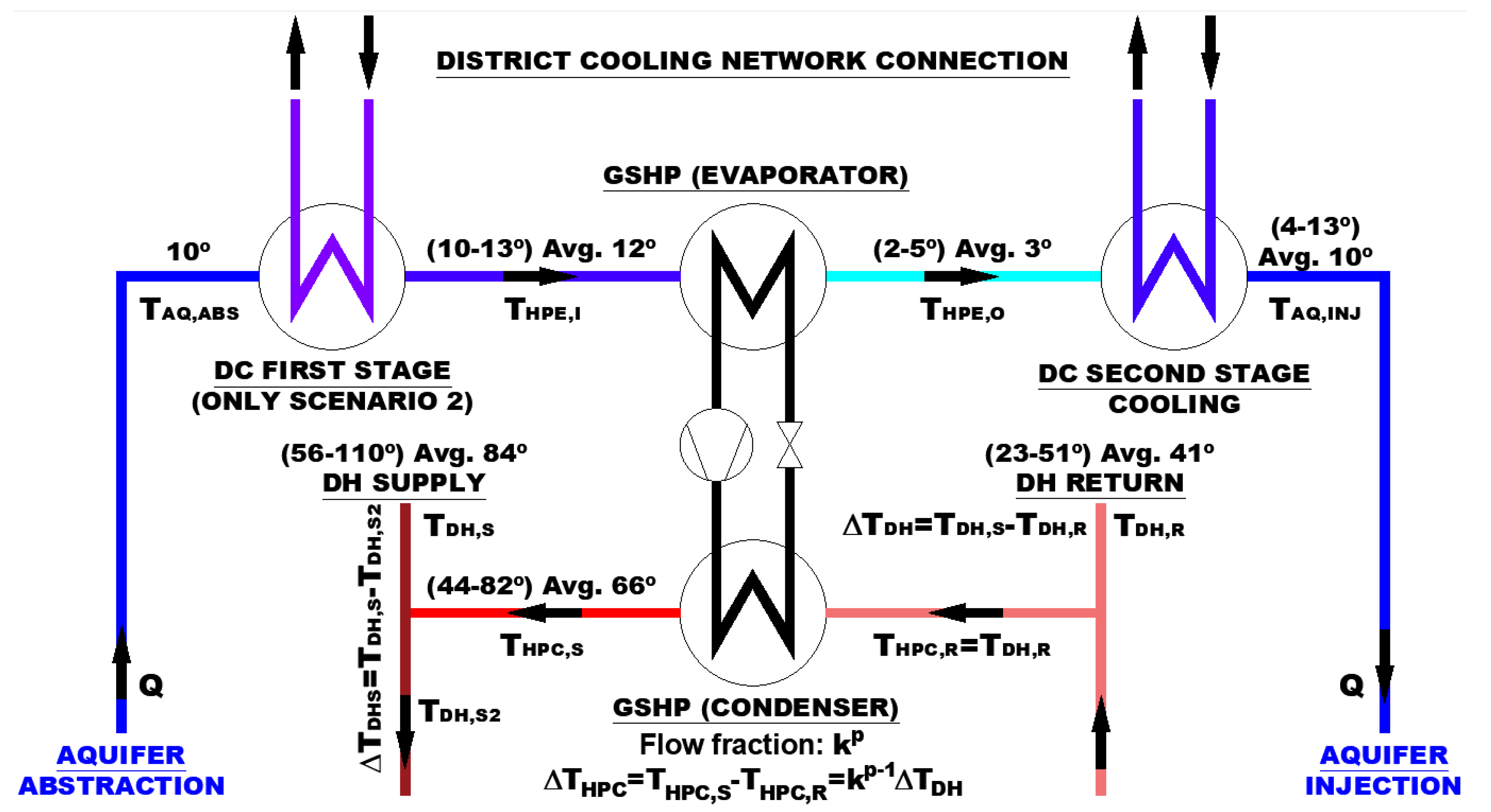
2.2. ATES–GSHP Integration for District Heating and Cooling

A ground-source heat pump (GSHP), operating with an abstraction and injection well (well doublet) was considered. The condenser side of the heat pump is connected to DH network while the evaporator side is connected to aquifer pumping stream.

In the base (first) scenario, the ATES pumping flow path encounters two serial exchangers—HP evaporator and cooling for DC network. In the second scenario before the HP evaporator, a precooling exchanger is added, providing a first stage cooling to the DC network. As will be shown in the result section, with this configuration the DC demand can be more efficiently covered and GSHP efficiency (COP) can be improved since heat pump inlet temperature increases several degrees after a precooling exchanger. ATES–GSHP integration within the existing DH–DC networks is depicted in the general scheme presented in Figure 3, where temperature values illustrate the second scenario setup.

2.3. Modeling Tools and Methods

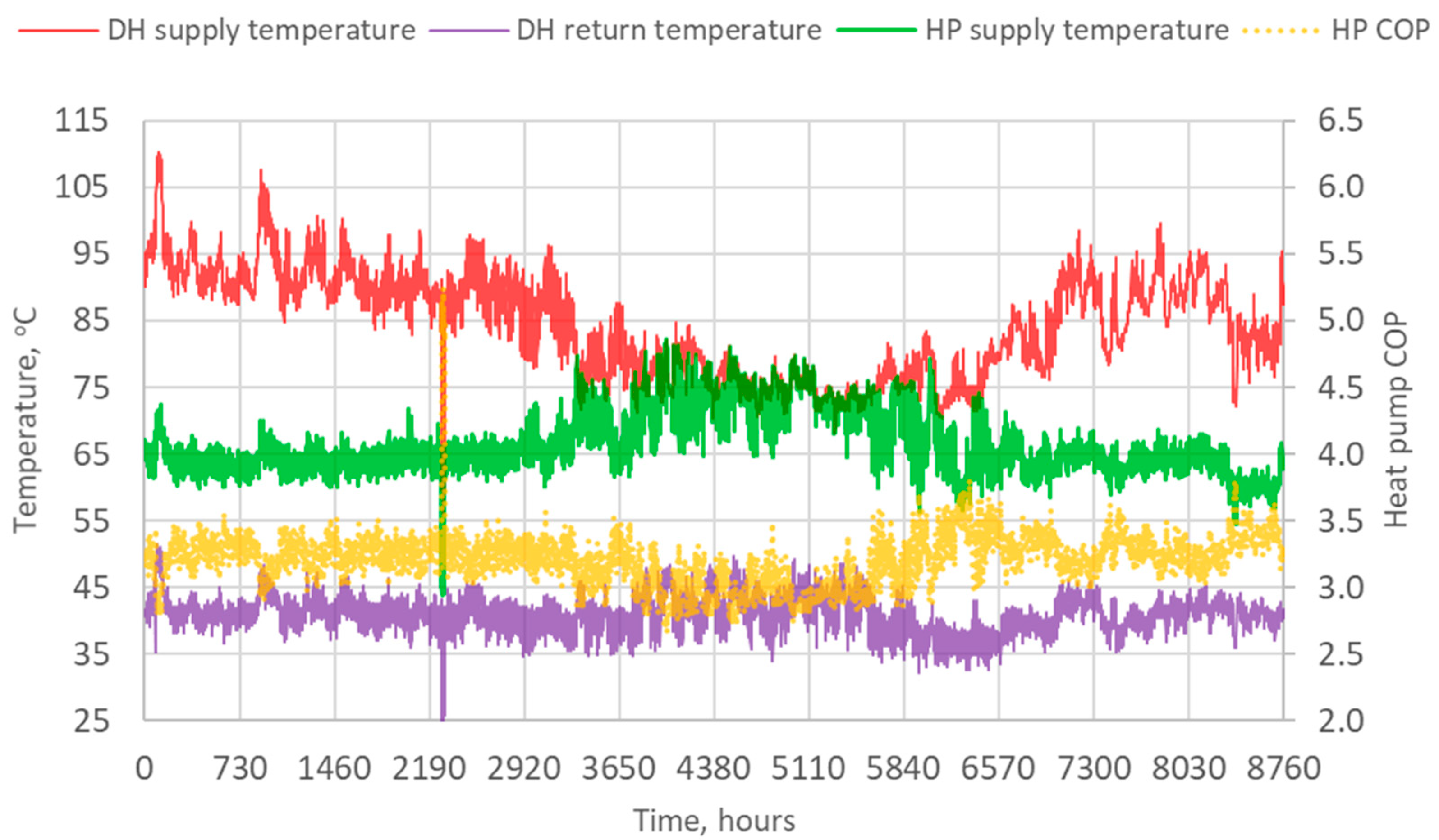
2.3.1. GSHP Utilization for District Heating

Generally speaking, GSHP is utilized to recover and upgrade all excess heat proceeding from the DC network and inject it in DH network. In this context ATES is utilized for balancing the energy system and mitigating the variability and no-coincidence of the simultaneously dispatched heating and cooling loads. For this purpose, heat pump supply temperature is calculated, based on the demanded power fraction k (the ratio between heat supplied by the heat pump and total heat demanded in the DH branch). The flow fraction recirculated through HP condenser can be calculated as: k^p, where 0 ≤ p ≤ 1 is additional exponent parameter, thus the ratio between heat pump condenser ∆T_HPC and total ∆T_DH of DH network is k^1-p. Therefore, for each hour n, given that T_DH,R,n and T_DH,S,n are DH return and supply temperatures respectively, the heat pump supply temperature T_HPC,S,n can be calculated as follows:

$$T_{HP,S,n}=T_{DH,R,n}+\left(T_{DH,S,n}-T_{DH,R,n}\right)k^{1-p}\Rightarrow \Delta T_{HPC,n}=\Delta T_{DH,n}{k}^{1-p}$$

(1)

The resulting supply temperature T_DH,S2,n after mixing can be calculated as:

$$T_{DH,S2,n}=T_{DH,R,n}+\left(T_{DH,S,n}-T_{DH,R,n}\right)\left(k^p-k\right)\Rightarrow \Delta T_{DH,S,n}=\Delta T_{DH,n}\left(k^p-k\right)$$

(2)

In the present case study, the exponential parameter p was chosen to equal 0.6. It can be observed that there is a significant advantage in partial load operation, since there is no need to increase HP supply temperature as high as DH supply, thus boosting the COP. For example, for power fraction k = 0.4 and ∆T_DH = 40 °C, the GSHP should elevate DH return temperature by roughly 28 °C instead of 40 °C. After mixing with the supply DH flow, the maximum temperature drop of the flow ∆T_DHS is ≈ 7 °C.

2.3.2. COP_H Estimation Model

For industrial and large-scale processes, multiple HP units in serial connection increase overall system efficiency, and therefore the Lorentz COP [9,18] would describe more accurately the behavior of the HP configuration, since it takes into account the logarithmic mean temperature of the sink and source, as well as both inlet and outlet temperatures of the condenser and evaporator. According to Reinholdt et al. [18], the maximum theoretical COP of a heat pump can be estimated by calculating Lorentz COP, defined as follows:

$$CO{P}_{Lor}=\frac{T_{lm,H}}{T_{lm,H}-T_{lm,L}}, \mathrm{where} T_{lm,H}=\frac{T_{HPC,S}-T_{HPC,R}}{ln\left(\frac{T_{HPC,S}}{T_{HPC,R}}\right)}; T_{lm,L}=\frac{T_{HPE,O}-T_{HPE,I}}{ln\left(\frac{T_{HPE,O}}{T_{HPE,I}}\right)}$$

(3)

In Equation (3), T_lm,H and T_lm,L are, respectively, the logarithmic mean temperature of the sink and source, where notations HPC and HPE stand for heat pump’s condenser and evaporator temperatures, while notations I/O stand for inlet/outlet temperatures of the evaporator and S/R stand for supply/return temperatures of the condenser (all values expressed in Kelvin). Based on the best industrial refrigeration systems, Reinholdt et al. [18] suggested values for Lorentz efficiency between 50% and 60% of the maximum Lorenz COP calculated with Equation (3). In our case study, a more conservative value of 45% was adopted.

2.3.3. GSHP Utilization for District Cooling

As mentioned previously, part of DC demand can be produced by free cooling in a first stage cooling exchanger located at the beginning of ATES pumping flow. After that, GSHP is utilized in the second place for simultaneously cooling the ATES flow in the evaporator as well as supplying heat to DH network in the condenser (see Figure 3). Finally, second stage cooling is applied, and groundwater is injected into the aquifer.

For each hour of operation, it is crucial to determine the exact aquifer pumping flow rate Q [m³/s] since there is constraint for daily pumping of 2500 m³/day. Due to this limitation, the maximum heat output of the GSHP condenser is limited to 1.4 and 1.6 MW in scenario 1 and 2 respectively, and pumping flow rate is calculated according to the iterative algorithm developed below.

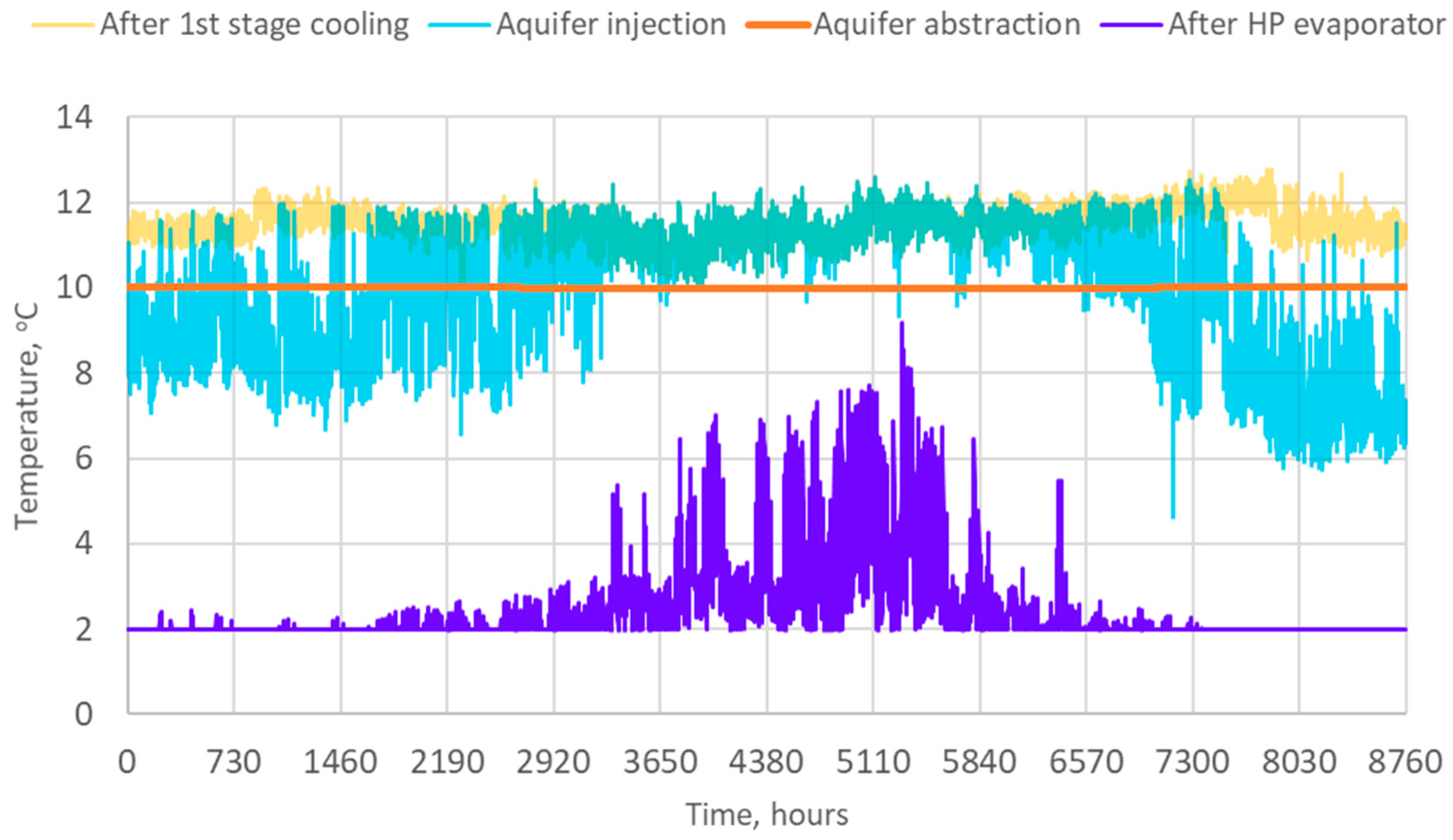
2.3.4. Computation of ATES Hourly Pumping Rate

Since there are several exchangers (two and three, respectively, for scenario 1 and 2) in the ATES flow path, the minimum needed pumping flow rate is proposed to be estimated iteratively. If Φ_heat,n and Φ_cool,n are, respectively, heating and cooling demand to be covered in hour n, as the first estimation of the pumping flow can be taken the maximum flow needed either for heating or cooling (notations according to Figure 3):

$$\begin{gathered} Step 1: Q_n=max\left\{\frac{\left(1-\frac{1}{CO{P}_n}\right){\varnothing }_{heat,n}}{S_{VC,wat}\left(T_{HPE,I,n}-T_{HPE,O,n}\right)};\frac{{\varnothing }_{cool,n}}{S_{VC,wat}\left(T_{HPE,I,n}-T_{AQ,ABS,n}+T_{AQ,INJ,n}-T_{HPE,O,n}\right)}\right\} \\ {T}_{HPE,I,n}=T_{AQ,ABS,n} \left(in sc. 1\right) ; T_{HPE,I,n}=max\left\{T_{AQ,ABS,n};T_{DC,R,n}-\Delta T_{min}\right\} \left(sc. 2\right) \\ {T}_{AQ,INJ,n,max}=T_{DC,R,n}-\Delta T_{min} ;T_{HPE,O,n,min}=2°C; S_{VC,wat}=4.19 MJ/m^{3}K \end{gathered}$$

where ΔT_min = 2 °C is the minimum pinch point difference in cooling exchangers and ΔT_HPE,O,n,min = 2 °C is the minimum temperature after the GSHP evaporator. COP_n is calculated with Equation (3), assuming average values for T_HPE,O = 10 °C (12 °C for scenario 2), T_HPE,O = 2 °C (3 °C for scenario 2). Once the first estimation for Q_n is known, it is possible to calculate separately all exchangers within the ATES flow path, in both scenarios 1 and 2, as follows.

Scenario 1: Recalculation of temperature after HP evaporator:

$$Step 2: T_{HPE,O,n}=T_{HPE,I,n}-\frac{\left(1-\frac{1}{CO{P}_n}\right){\varnothing }_{heat,n}·Q_n}{S_{VC,wat}}$$

Scenario 2: Recalculation of first and second stage cooling demands:

$$Step 2: {\varnothing }_{cool-1stage,n}=Q_n{S}_{VC,wat}\left(T_{HPE,I,n}-T_{AQ,ABS,n}\right)$$

$$T_{HPE,O,n}=T_{HPE,I,n}-\frac{\left(1-\frac{1}{CO{P}_n}\right){\varnothing }_{heat,n}·Q_n}{S_{VC,wat}}$$

$${\varnothing }_{cool-2stage,n}=min\left\{Q_n{S}_{VC,wat}\left(T_{HPE,I,n}-T_{AQ,INJ,n}\right);{\varnothing }_{cool,n}-{\varnothing }_{cool-1stage,n}\right\}$$

$${\varnothing }_{cool,n}={\varnothing }_{cool-1stage,n}+{\varnothing }_{cool-2stage,n}$$

The ATES flow is recalculated again in Step 1, and if the new value deviates more than a predefined threshold from the previous one (in this case a 5% threshold is adopted), then the whole loop (Step 1/Step 2) is repeated.

2.3.5. Calculation of ATES Pumping Power Demand

The required pumping power [kW] for ATES operation can be calculated on an hourly basis, assuming overall pressure drop in the line ∆p = 600 kPa and standard pumping efficiency η = 0.55 [19], as follows:

$$P_{ATES,n}=\frac{Q_n\Delta p}{\eta }$$

(4)

2.3.6. Calculation of Pumping Power Demand to DH–DC Network

Similarly, pumping power [kW] to provide DH–DC through the GSHP condenser/evaporator respectively can be calculated hourly, assuming overall pressure drop between supply and return lines ∆p_DH = ∆p_DC = 250 kPa [20] and standard pumping efficiency η = 0.55 [21], as follows:

$$P_{HPC-to-DH,n}=\frac{Q_{HPC,n}\Delta p_{DH}}{\eta } ; P_{HPE-to-DC,n}=\frac{Q_{HPE,n}\Delta p_{DC}}{\eta }$$

(5)

where

$$Q_{HPC,n}=\frac{{\varnothing }_{supplied-heat,n}}{S_{VC,wat}\left(T_{HPC,S,n}-T_{DH,R,n}\right)} ; Q_{HPE,n}=\frac{{\varnothing }_{cool-1stage,n}+{\varnothing }_{cool-2stage,n}}{S_{VC,wat}\left(T_{DC,R,n}-T_{DC,S,n}\right)}$$

(6)

The volumetric heat capacity of water S_VC,wat used was 4.19 and 4.1 MJ/m³K, respectively, for cooling and heating operation.

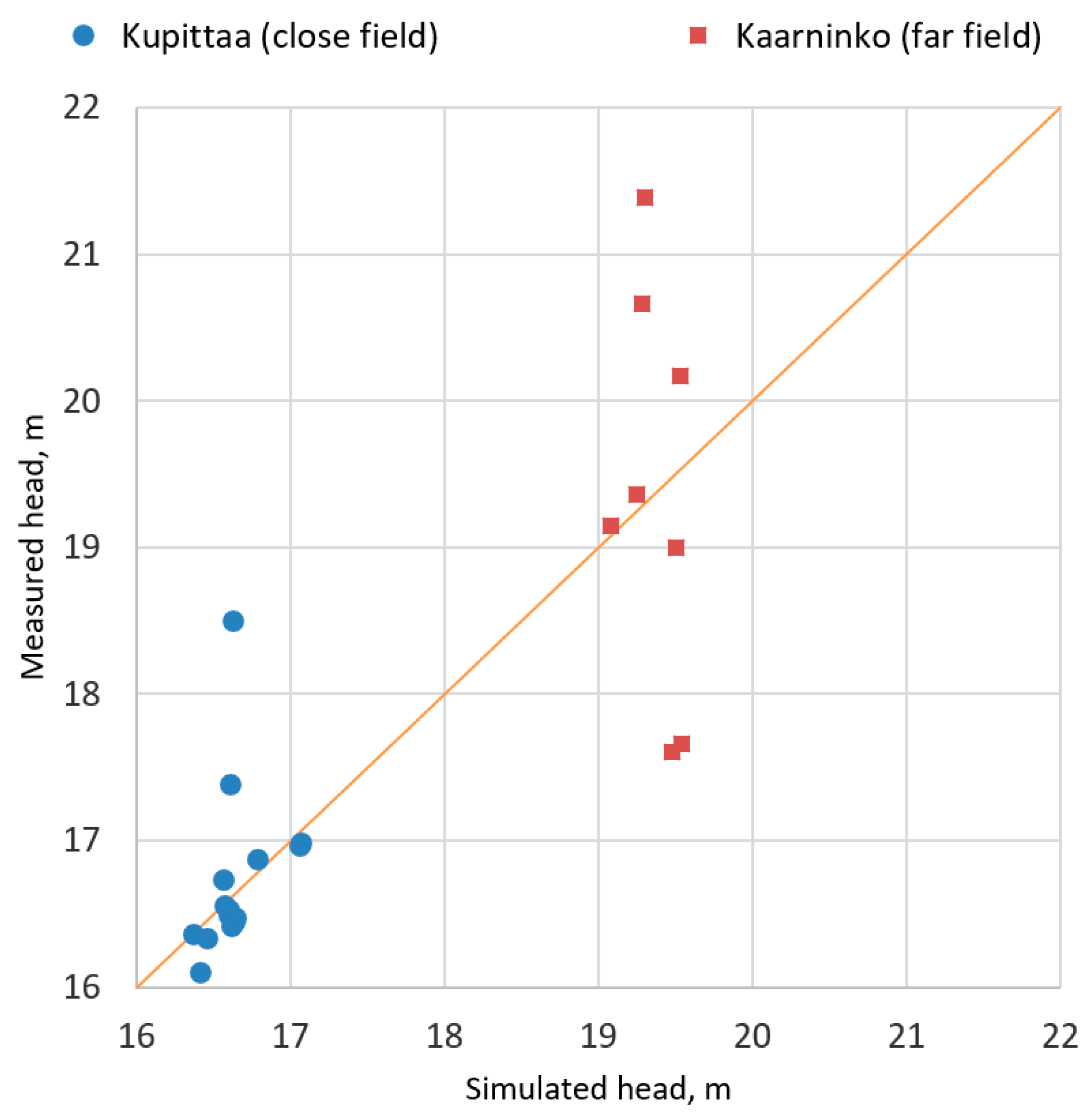
2.3.7. Numerical Model and Its Calibration for Steady State

The groundwater model is set up utilizing the finite difference code MODFLOW [12] with ModelMuse environment [22]. In ModelMuse, the aquifer is discretized with a 100 x 100 m square cell grid, covering a physical extension of about 20 km², delimited between the Aura River to the northwest and the Baltic Sea to the southwest. Southeast and northeast borders are assumed as no-flow boundaries (see Figure 4).

Groundwater model calibration for steady state was carried out taking into account the long-term statistical data for 15 observation wells in the Kupittaa area and eight observation wells in Kaarninko. Calibration was done according to the procedure developed by Todorov et al. [23], by using root mean squared error (RMSE) [24] and mean absolute error (MAE) [25] for the close field (Kupittaa) and far field (Kaarninko). As seen in Figure 5, the results of Kaarninko (far-field area) were more dispersed (calculated RMSE = 1.32 m/MAE = 1.07 m), since our model is intended to present better correlation between measured and simulated values (RMSE = 0.54 m/MAE = 0.29 m) within the close-field calibration. In most of Kupittaa’s observation wells, this difference was within the margins of the measured long-term standard deviation. A typical horizontal hydraulic conductivity for sand/gravel aquifer was selected: K = 5 × 10⁻⁵ m/s (Luoma [26]), and during model calibration was adjusted to 5 × 10⁻⁴ m/s for the area containing the observation wells (small black rhombs in Figure 4 delimited by circles). The value of vertical hydraulic conductivity was chosen as K_z = 0.1K. Typical values were also utilized for storativity (S = 1 × 10⁻⁵), porosity (n = 0.25) and recharge rate of R = 1.3 × 10⁻⁸ m/s [26].

In Figure 4, the calibrated groundwater model and its steady state solution are depicted, where iso-lines represent groundwater head in meters while the color grid represent elevation between blue (min. elevation, 0.3 m above sea level) and red (max. elevation 59.6 m). As seen in Figure 4, the natural groundwater flow moves from the Kaarninko area (highest hydraulic heads 19–20 m) towards the Kupittaa area (hydraulic heads 16–17 m), and finally reaches the lowest hydraulic boundaries represented by the Aura River and Baltic Sea.

2.4. Technoeconomic Evaluation of GSHP–ATES

Based on hourly calculations, different technical variables are computed, like the annual energy generation for heating/cooling, the electricity consumption and the average daily ATES pumping rate.

Table 2. Technical variables of ATES.

Variables	Units	Comments
GSHP supply temperature	°C	Depending on demanded power fraction, Equation (1)
GSHP COP	-	Depending on GSHP source and sink temperatures, Equation (3)
ATES flow rate Q	m3/s	Calculated according to the algorithm exposed in 2.3.2
GSHP electric power demand	MW	Based on HP heat load covered and COP
Electric power demand for ATES pumping	kW	Based on the computed flow rate Q, assumed pressure drop and efficiency (Equation (4))
Electric power demand for DH–DC pumping	kW	Based on the computed flow rate for each network, assumed pressure drop and efficiency (Equation (5))
Daily ATES flow rate	m3/day	Average daily ATES flow rate
Annual heating demand	MWh	Heating demand covered by GSHP
Annual cooling demand	MWh	Cooling demand covered by ATES system (first/second stage)
Annual GSHP demand	MWh	Electricity demand of GSHP
Annual pumping demand	MWh	Pumping demand of ATES, DH and DC operation

lists the relevant ATES technical variables.

A cost database regarding various energy generation technologies was used (after Nielsen et al. [27,28]), as well as prices for ATES well drilling, heat exchangers, and piping (Drenkelfort et al. [29]) for estimating the investment cost. Based on the annuity method, the energy generation cost is calculated, assigning annual investment payments (annuity) and assuming 5% interest rate as well as the investment lifetime of 20 years (Nielsen et al. [27]). The operation and maintenance (O&M) costs (1% of investment) are also included within the overall annual cost, as well as the electricity cost for GSHP and pumping (given electricity price of 100 €/MWh, including taxes, transfer and distribution fees [30]). The economic evaluation was developed according to Todorov et al. [23], including the calculation of the following variables listed in

Table 3. Variables for economic evaluation.

Variables	Units	Comments
Overall investment cost	€	Geological survey, cost of GSHP, exchangers, drilling and piping
Annuity factor	-	Computed for 20 years lifetime and 5% interest rate
Investment cost (annuity)	€	Calculated as overall investment cost times annuity factor
Fixed annual O&M costs	€	1% of overall investment cost
Electricity annual cost	€	Electricity cost of GSHP and pumping
Overall annual cost	€	Annuity + O&M costs + electricity cost
Specific energy cost	€/MWh	Overall annual cost per total thermal energy generation

.

3. Results and Discussion

3.1. Technoeconomic Analysis

The main technical parameters of ATES operation for both studied scenarios are shown in

Table 4. ATES system technical parameters.

Relevant Parameters of ATES Operation	Annually		Summer		Winter
Annual/seasonal results for scenarios 1/2	Sc. 1	Sc. 2	Sc. 1	Sc. 2	Sc. 1	Sc. 2
ATES period duration, weeks	52	52	26	26	26	26
Pre-cooling/heating/cooling power, MW	-/1.43/1	0.3/1.63/1.3	-	-	-	-
Average water flow, m3/day	2492	2496	2452	2559	2531	2434
Average abstraction temperature, °C	10.0	10.0	10.0	10.0	10.0	10.0
Average injection temperature, °C	10.0	10.0	10.4	11.0	9.5	8.9
Average temperature before GSHP, °C	10.0	11.5	10.0	11.5	10.0	11.6
Average temperature after GSHP, °C	2.1	2.5	2.2	3.0	2.0	2.0
Average GSHP supply temperature, °C	65.4	66.5	68.1	69.3	62.6	63.8
Average DH return temperature, °C	40.9	40.9	40.5	40.5	41.4	41.4
Average GSHP COP (heating mode)	3.14	3.21	3.08	3.14	3.20	3.27
Heating demand, MWh	67,971		16,761		51,210
Heat demand covered by GSHP, MWh	12,315	13,882	6034	6723	6281	7159
Heating demand covered by GSHP, %	18%	20%	36%	40%	12%	14%
Cooling demand, MWh	12,382		7944		4439
First stage cooling covered, MWh	-	1605	-	780	-	825
Second stage cooling covered, MWh	8331	8006	4279	4454	4052	3551
Total cooling demand covered, MWh	8331	9611	4279	5234	4052	4377
Total cooling demand covered, %	67%	78%	54%	66%	91%	99%
Electricity demand (GSHP), MWh	3934.2	4334.5	1964.4	2138.9	1969.8	2195.6
Electricity demand (ATES pump.), MWh	275.6	276.1	135.2	141.1	140.4	134.9
Electricity demand (HP-DH pump.), MWh	57.7	62.1	24.8	26.5	33.0	35.7
Electricity demand (HP-DC pump.), MWh	130.7	150.5	66.6	81.3	64.1	69.3
Total electricity demand, MWh	4398.2	4823.2	2191.0	2387.7	2207.2	2435.5

. It can be acknowledged that even with 5%–6% of peak heat power for scenario 1 and 2, the GSHP coverage ratio is 18%–20% of the annual heating demand. Moreover, an important advantage of scenario 2 is shown when comparing a cooling demand covered by ATES. The scheme with two cooling exchangers in scenario 2 allows 78% coverage of DC demand annually (compared to 67% in scenario 1), from which the first stage cooling represents roughly one sixth.

The estimation of economic feasibility parameters and the production cost of thermal energy are shown in

Table 5. Economic parameters of GSHP–ATES.

Investment Cost.	Price	Sc. 1 (Units)	Sc. 2 (Units)	Total Scenario 1	Total Scenario 2
Subsurface study, geological report and pumping tests, €/u	30,000	1	1	30,000	30,000
Ground-source heat pump, €/kW	300	1.43	1.63	429,000	489,000
Heat exchangers, €/kW	35	2.43	3.23	85,050	113,050
Pumping well (including equipment and pump), €/u	170,000	8	8	1,360,000	1,360,000
Connection pipes, €/m	250	1300	1300	325,000	325,000
Overall investment cost, €				2,229,050	2,317,050

and

Table 6. Energy production cost.

Annuity Method	Scenario 1	Scenario 2
Annuity factor (interest rate 5%, 20 years lifetime)	0.0802
Investment cost (annuity), €	178,865 €	185,786 €
Fixed annual O&M cost, €	22,291 €	23,153 €
Electricity annual cost, €	439,820 €	482,324 €
Overall annual cost, €	640,976 €	691,263 €
Specific energy cost, €/MWh	31.05 €/MWh	29.43 €/MWh

respectively. The resulting thermal energy production cost in scenario 2 is slightly below 30 €/MWh. Overall investment cost is around 2.3 million €: 26% corresponds to GSHP/exchangers and 73% is related to the underground components (connection pipes and wells), figures close to similar ATES realization in Germany (Schüppler et al. [31]). The specific investment cost per installed heat pump capacity is 1.6/1.4 €/W for scenario 1 and 2 respectively, values comparable to the 1.8 €/W reported for a similar ATES system in a Belgian hospital (Vanhoudt et al. [32]).

Additionally, scenario 2 is investigated with more details, as follows. GSHP COP is 3.2 on average, slightly improving to 3.3 during the winter due to lower GSHP supply temperature (64 °C on average), while, during the summer, GSHP covers a higher heat fraction and the average supply temperature increases to 69 °C (see Figure 6).

ATES operation is based on energy conversion using electricity to cogenerate heating and cooling in a single operation. GSHP is the principal electricity consumer accounting for 90% of the annual demand, followed by ATES pumping (6%) as well as pumping needed to inject HP supply energy to DH–DC networks—respectively 1% and 3%. This is important to acknowledge since total electricity demand (4.8 GWh/a) has a significant impact on the annual cost, and, consequently, on the specific cost of generated heating and cooling energy, as seen in Table 6. The ATES system is well balanced, as seen from the average injection and abstraction temperatures that are both equal to the aquifer’s undisturbed temperature of 10 °C. Moreover, the system is balanced in terms of energy, as shown in Table 4, since the annual heat demand covered is equal to cooling demand covered plus GSHP power demand (13.9 GWh). Figure 7 depicts the annual variation of all temperatures along the ATES flow path: abstraction, after first stage cooling, after GSHP evaporator, and finally injection.

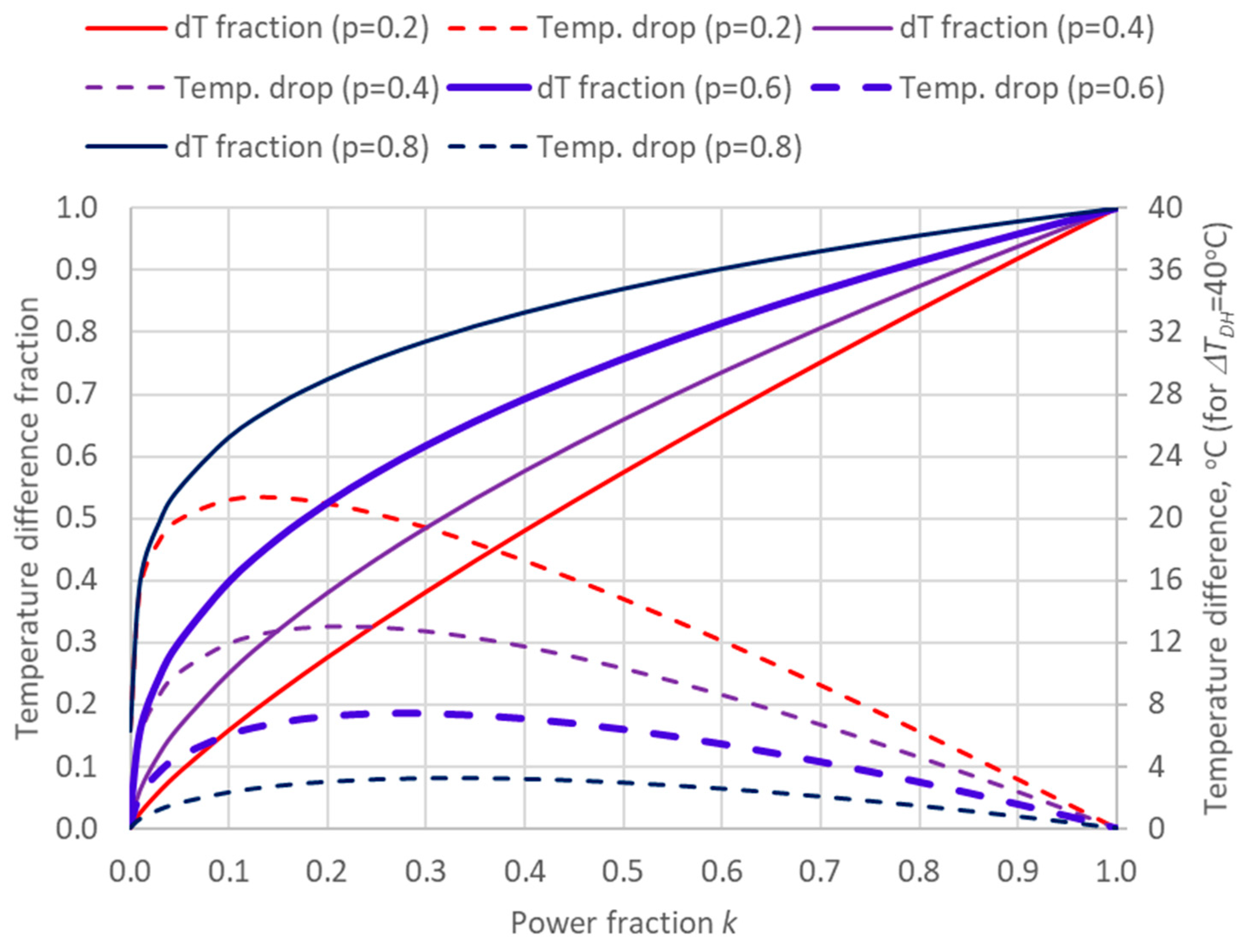
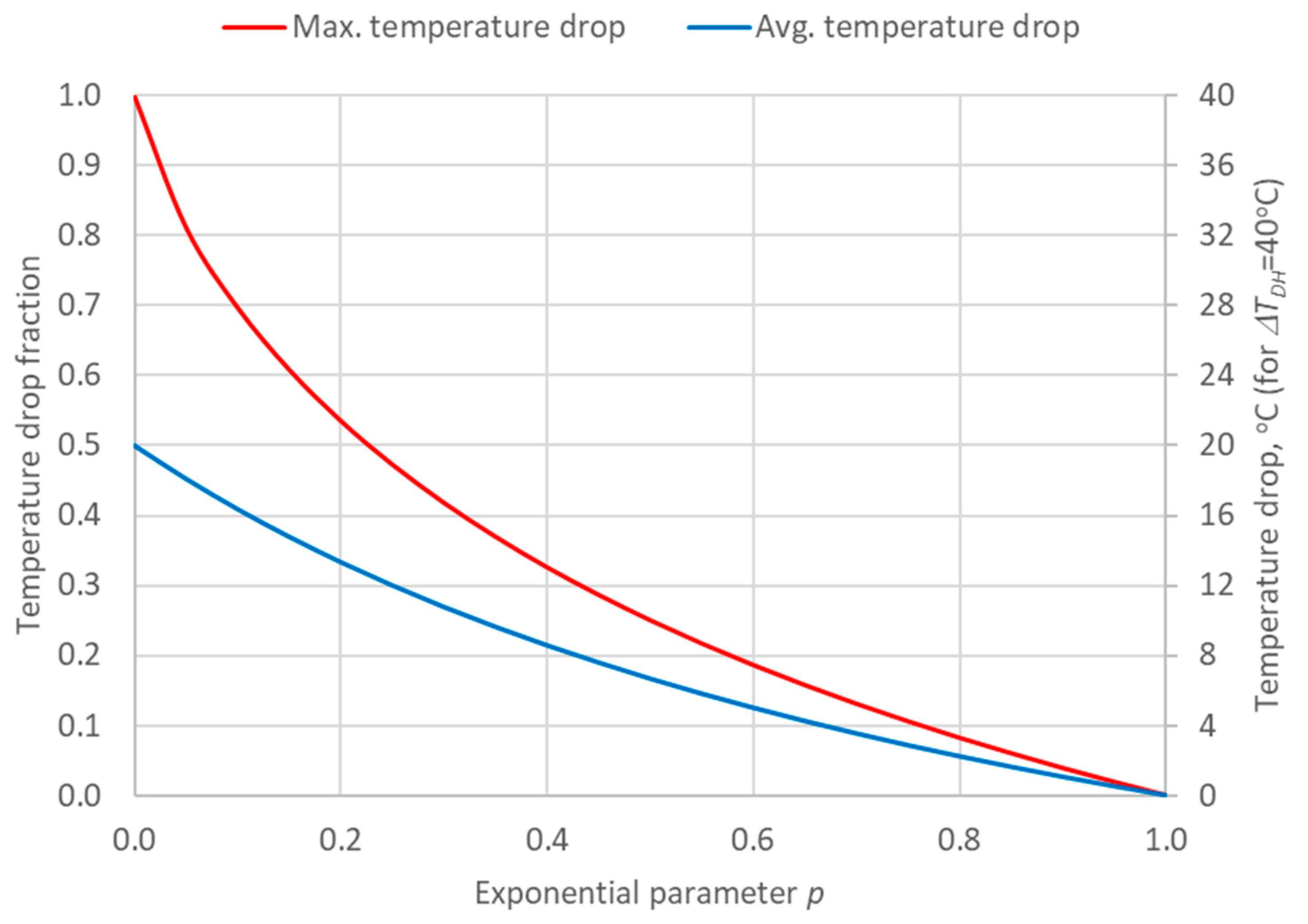
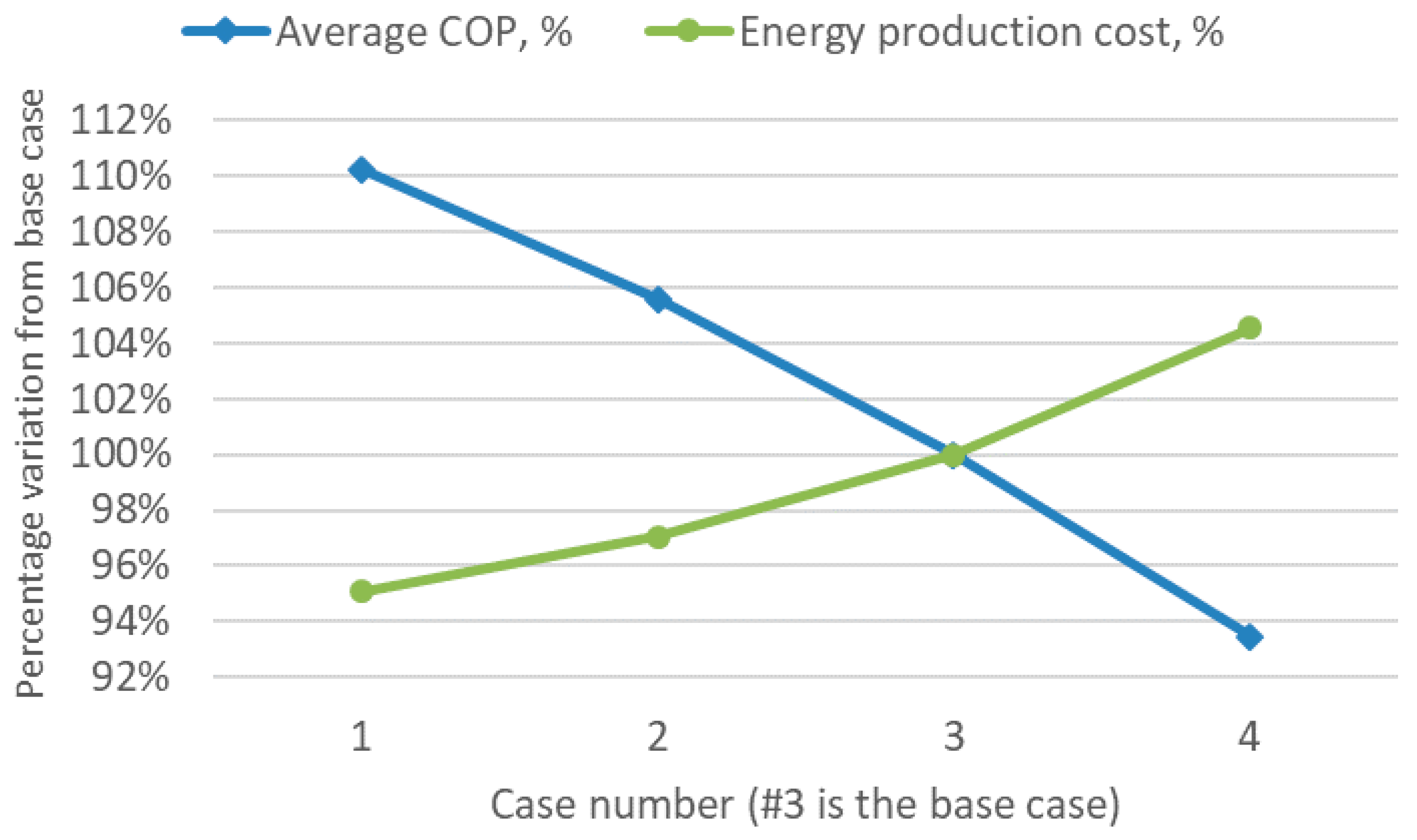
3.2. Sensitivity Analysis of the System’s Operation

As shown in Table 6, about 70% of energy production cost is related to electricity consumption, of which the GSHP accounts for around 90%. The heat pump’s COP is an important variable to consider in order to boost the system’s efficiency and decrease cost. That is why, in this section, a sensitivity analysis will be performed regarding COP and energy production cost, and how they depend on the exponent parameter p. The effect of varying p within the interval [0;1] is that, e.g., for p = 1, flow recirculated through GSHP condenser is directly proportional to power fraction k, and thus heat pump supply temperature should be equal to DH supply temperature. Figure 8 plots a ∆T_HPC/∆T_DH fraction of GSHP condenser calculated with Equation (1) and a temperature drop fraction after heat pump junction ∆T_DH,S/∆T_DH calculated with Equation (2) for different values of p = 0.2, 0.4, 0.6, 0.8. The comparative thermal effect for ∆T_DH = 40 °C is illustrated in the secondary vertical axis. From Figure 8, it can be seen that, for lower values of p, the GSHP has higher efficiency when working at lower power fractions (e.g., during the winter period) since HP supply temperature is not so high as DH supply. The drawback is that, after HP junction, DH supply temperature T_DH,S2 can also present an important temperature drop ∆T_DH,S (e.g., red dashed curve, for p = 0.2). It is also interesting to explore what is the maximum ∆T_DH,S for each p within the interval [0;1]. Let’s define the following function f(k), as the ratio between ∆T_DH,S and ∆T_DH, according to Equation (2):

$$f\left(k\right)=k^p-k\Rightarrow f^{\prime }\left(k\right)=\frac{df}{dk}=p{k}^{p-1}-1$$

(7)

As seen from Figure 8, in the interval [0;1], f(k) has one maximum, which can be found where the function’s first derivative is zero:

$$\begin{gathered} 0=f^{\prime }\left(k\right)=p{k}^{p-1}-1\iff p{k}^{p-1}=1\Rightarrow k_{max}=p^{\frac{1}{1-p}} \\ \Rightarrow f_{max}=f\left(k_{max}\right)=p^{\frac{p}{1-p}}-p^{\frac{1}{1-p}}=p^{\frac{1}{1-p}}\left(p^{-1}-1\right) \end{gathered}$$

(8)

Similarly, it is possible to calculate the average value of f(k) within [0;1] as:

$$f_{avg}={{\displaystyle \int }}_0^{1}f\left(k\right)={{\displaystyle \int }}_0^1{k}^p-k=\frac{1}{1+p}-\frac{1}{2}$$

(9)

The results for f_max and f_avg calculated respectively with Equations (8) and (9) are presented in Figure 9.

As previously noticed, and also presented in Figure 8 and Figure 9, for low values of p, the temperature drop after HP junction can increase significantly. Moreover, when p = 0.2, for the maximum and average temperature drop, the fraction is as high as 0.53 and 0.33 of ∆T_DH respectively, while for p = 0.8 the possible gains in low power fraction are quite limited. Therefore, a sensitivity analysis for scenario 2 was performed, for four different values of p:

• Case 1: p = 0.2
• Case 2: p = 0.4
• Case 3: p = 0.6 (base case, blue thick curves in Figure 8)
• Case 4: p = 0.8

All cases are simulated on an hourly basis, with the same constraint for ATES average daily pumping flow, and the annual results are listed in

Table 7. Sensitivity analysis based on four cases (case 3 is the base case).

Relevant ATES Parameters.	C1: p = 0.2	C2: p = 0.4	C3: p = 0.6	C4: p = 0.8
Peak pre-cooling/heating/cooling power, MW	0.3/1.57/1.3	0.3/1.6/1.3	0.3/1.63/1.3	0.3/1.7/1.34
Annual heat demand supplied by GSHP, MWh	13,418	13,650	13,882	14,419
Annual cooling demand supplied, MWh	9551	9577	9611	9659
Average GSHP supply temperature, °C	57.2	61.1	66.5	74.1
Average GSHP COP (heating mode)	3.53	3.38	3.21	3.00
Average drop in DH supply temperature, °C	19.1	11.6	6.4	2.7
Cost per MWh of heating/cooling energy	27.99 €	28.56 €	29.43 €	30.77 €

. By decreasing p, the average GSHP supply temperature also decreases, while the average COP increases, and vice versa. From Table 7, it also can be seen that the higher the COP, the lower GSHP heat capacity needed, since the fraction supplied by the HP compressor is lower. The latter also explains why the annual heat demand covered is lower for high COP, while the annual cooling demand covered remains stable among the four cases.

The percentage variations compared to the base case 3 are plotted in Figure 10. It is important to notice how the energy production cost decreases as COP increases. On the other hand, an important drawback for cases 1 and 2 is the high temperature drop in DH supply temperature, 19.1 °C and 11.6 °C respectively, which is a confirmation that case 3 is a reasonable trade-off between the system’s efficiency, economic feasibility, and technical constraints.

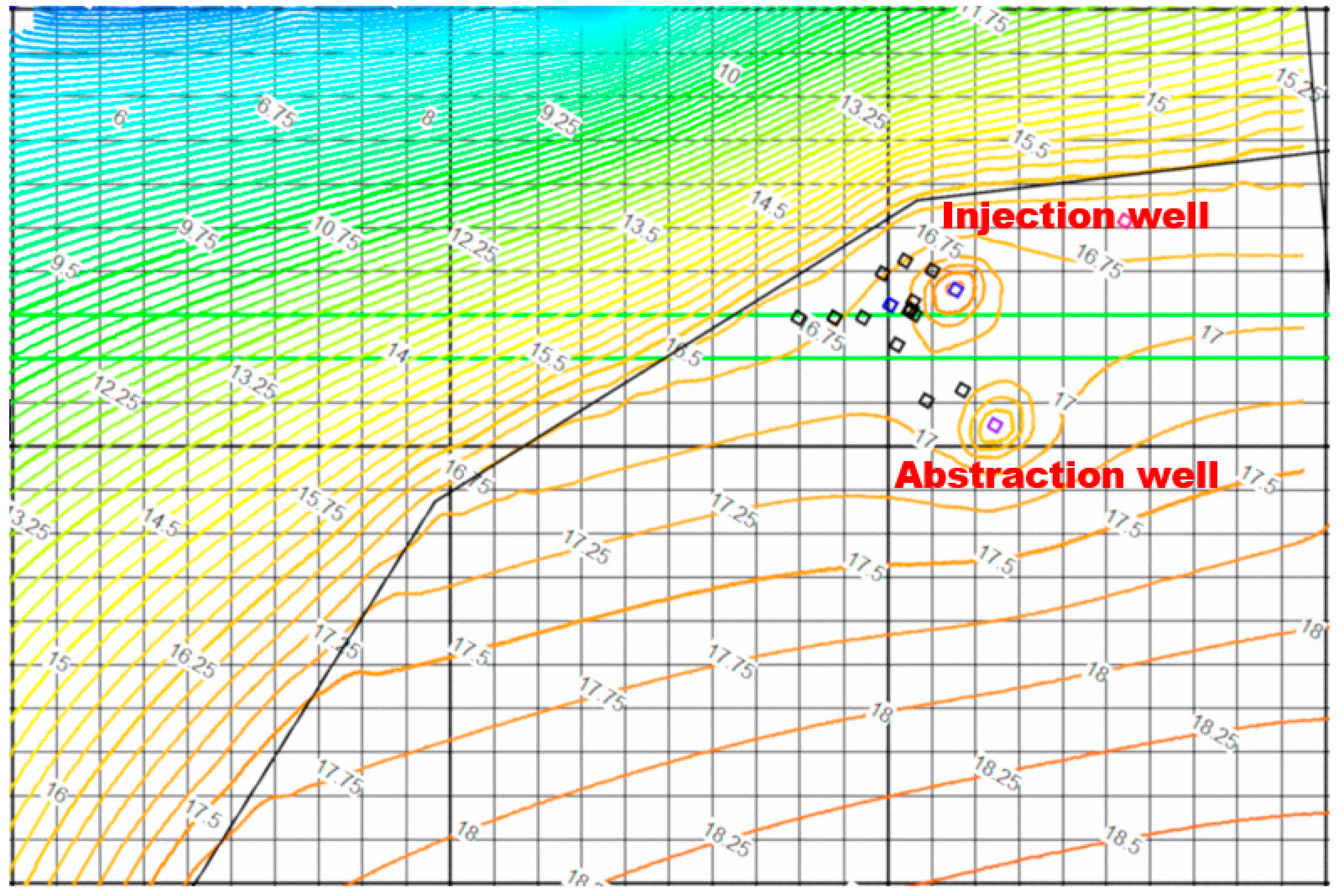
3.3. Impact on Groundwater Areas

Although the undisturbed aquifer temperature is as high as 10 °C, first stage cooling can be used in 8736 out of 8760 h, and annually it represents 17% of cooling demand covered by ATES (about one sixth of 9.6 GWh). This configuration also increases the temperature before GSHP evaporator by 1.5 °C on average, which improves the COP and enhances the heat pump’s capacity in the evaporator as well. The average injection temperature lies in a narrow range of roughly 10 ± 1 °C (see Table 4), which justifies one-way ATES operation and, consequently, the thermal impact on the aquifer remains very limited.

The long-term hydraulic impact was simulated in MODFLOW by taking a weekly-based average for ATES pumping rate and defining 52 × 20 = 1040 stress periods. The result after 20 years of one-way operation is presented in Figure 11, where hydraulic head is represented by iso-lines with resolution of 0.25 m. In order to mitigate the hydraulic impact of pumping, the injection well is placed downstream while the abstraction well is located upstream (Figure 11). The maximum simulated drawdown is 1.28 and 1.17 m for summer and winter operation respectively, which corresponds to 5.0 and 4.7 m inside the pumping well. The overall impact of ATES pumping vanishes at about 500 m from each well, thus it does not affect the surrounding groundwater areas in a significant way.

4. Conclusions

The presented case study was successful in demonstrating and developing a mathematical model for system’s management: calculation of HP recirculation flow, estimation of heat pump COP, as well as an algorithm for computation of ATES pumping flow rate based on the capacity to cover heating and cooling demand in a single operation. Additionally, the system’s technoeconomic feasibility, efficiency, and the impact of GSHP–ATES operation on the nearby aquifer were evaluated. The groundwater model was developed and calibrated, utilizing different available data sources like the National Land Survey of Finland (NLSF), Finnish Environment Institute (SYKE), Geological Survey of Finland (GTK) and different tools such as MS Excel, QGIS and MODFLOW.

The dispatch of combined heating and cooling loads using annual data for an existing urban district in Finland was developed in tandem with the GSHP–ATES model. It presented an attractive economic outcome—competitive energy production cost around 30 €/MWh, far below 76.7 €/MWh, which was the average Finnish DH price in 2017 [33], as well as very limited long-term environmental impact on the nearby aquifer. The maximum drawdown within the pumping well was estimated as 5 m after 20 years of operation, and the overall hydraulic impact is limited to 500 m around the wells. Injection temperature deviates from undisturbed aquifer temperature at a level of about 1 °C on average, which is within the limits of Swiss (3 °C) and French (11 °C) legislation. Additional sensitivity analysis revealed that, by varying HP recirculation flow parameter (exponent parameter p), it is possible to influence the heat pump’s COP and the energy production cost. However, the only constraint to be considered is the temperature drop after the HP junction in the DH supply line, which in the base case resulted in 6.4 °C on average. The future transition to low district heating networks (Guzzini et al. [34]) by the introduction of heat pumps can eventually benefit from the proposed mathematical methodology due to its capability to find a trade-off between the energy production cost and the maximum allowed temperature drop introduced by the heat pump in the DH supply line.

The environmental assessment presented in this work was carried out using available hydrogeological data of the investigated groundwater area. The lack of reliable hydrogeological information at the present prefeasibility stage was a significant constraint for simplifying the groundwater model—the aquifer was assumed as uniform, isotropic and confined to the considered domain, and model calibration was performed only for steady state. Additional pumping tests and more detailed geological exploration would be needed as future steps.

Overall, ATES–GSHP systems prove to be a sustainable and efficient alternative to traditional thermal energy generation based primarily on fossil fuels, due to their ability to recycle heating and cooling loads using the subsurface as practically unlimited thermal storage. By dispatching annually balanced heating and cooling loads within integrated urban energy networks, major economic and technical improvements can be accomplished.

References

1. EUROSTAT. Renewable Energy for Heating and Cooling. Available online: https://ec.europa.eu/eurostat/web/products-eurostat-news/-/DDN-20200211-1?inheritRedirect=true&redirect=%2Feurostat%2F (accessed on 21 February 2020).
2. Pellegrini, M.; Bloemendal, M.; Hoekstra, N.; Spaak, G.; Andreu Gallego, A.; Rodriguez Comins, J.; Grotenhuis, T.; Picone, S.; Murrell, A.J.; Steeman, H.J. Low carbon heating and cooling by combining various technologies with Aquifer Thermal Energy Storage. Sci. Total Environ. 2019, 665, 1–10. [Google Scholar] [CrossRef]
3. Fleuchaus, P.; Godschalk, B.; Stober, I.; Blum, P. Worldwide application of aquifer thermal energy storage—A review. Renew. Sustain. Energy Rev. 2018, 94, 861–876. [Google Scholar] [CrossRef]
4. Hooimeijer, F.L.; Maring, L. The significance of the subsurface in urban renewal. J. Urban. 2018, 11, 303–328. [Google Scholar] [CrossRef] [Green Version]
5. Schmidt, T.; Pauschinger, T.; Sørensen, P.A.; Snijders, A.; Djebbar, R.; Boulter, R.; Thornton, J. Design Aspects for Large-scale Pit and Aquifer Thermal Energy Storage for District Heating and Cooling. Energy Procedia 2018, 149, 585–594. [Google Scholar] [CrossRef]
6. Bonte, M.; Stuyfzand, P.J.; Hulsmann, A.; van Beelen, P. Underground thermal energy storage: Environmental risks and policy developments in the Netherlands and European Union. Ecol. Soc. 2011, 16, 15. [Google Scholar] [CrossRef] [Green Version]
7. Haehnlein, S.; Bayer, P.; Blum, P. International legal status of the use of shallow geothermal energy. Renew. Sustain. Energy Rev. 2010, 14, 2611–2625. [Google Scholar] [CrossRef]
8. Paiho, S.; Saastamoinen, H.; Hakkarainen, E.; Similä, L.; Pasonen, R.; Ikäheimo, J.; Rämä, M.; Tuovinen, M.; Horsmanheimo, S. Increasing flexibility of Finnish energy systems—A review of potential technologies and means. Sustain. Cities Soc. 2018, 43, 509–523. [Google Scholar] [CrossRef]
9. Popovski, E.; Aydemir, A.; Fleiter, T.; Bellstädt, D.; Büchele, R.; Steinbach, J. The role and costs of large-scale heat pumps in decarbonising existing district heating networks—A case study for the city of Herten in Germany. Energy 2019, 180, 918–933. [Google Scholar] [CrossRef]
10. Soltani, M.; Kashkooli, F.M.; Dehghani-Sanij, A.R.; Kazemi, A.R.; Bordbar, N.; Farshchi, M.J.; Elmi, M.; Gharali, K.B.; Dusseault, M. A comprehensive study of geothermal heating and cooling systems. Sustain. Cities Soc. 2019, 44, 793–818. [Google Scholar] [CrossRef]
11. Fleuchaus, P.; Schüppler, S.; Godschalk, B.; Bakema, G.; Blum, P. Performance analysis of Aquifer Thermal Energy Storage (ATES). Renew. Energy 2020, 146, 1536–1548. [Google Scholar] [CrossRef]
12. Harbaugh, A.W. MODFLOW-2005, The U. S. Geological Survey Modular Ground-Water Model—The Ground-Water Flow Process; US Department of the Interior, US Geological Survey: Reston, VA, USA, 2005.
13. SYKE. Finnish Environment Institute/Suomen Ympäristökeskus. Available online: https://www.syke.fi/en (accessed on 14 April 2020).
14. Joronen, L. Groundwater Protection Plan for Turku, Kaarina and Rusko Orig. Title “Turun, Kaarinan ja Ruskon Pohjavesialueiden Suojelusuunnitelma”. Available online: https://www.turku.fi/sites/default/files/atoms/files/2010-turun_kaarinan_ja_ruskon_pohjavesialueiden_suojelusuunnitelma.pdf (accessed on 20 February 2020).
15. Bayer, P.; Attard, G.; Blum, P.; Menberg, K. The geothermal potential of cities. Renew. Sustain. Energy Rev. 2019, 106, 17–30. [Google Scholar] [CrossRef]
16. NLSF. National Land Survey of Finland. Available online: https://tiedostopalvelu.maanmittauslaitos.fi/tp/kartta?lang=en (accessed on 14 April 2020).
17. QGIS. QGIS—The Leading Open Source Desktop GIS. Available online: https://www.qgis.org/en/site/about/index.html (accessed on 12 March 2020).
18. Reinholdt, L.; Kristófersson, J.; Zühlsdorf, B.; Elmegaard, B.; Jensen, J.; Ommen, T.; Jørgensen, P.H. Heat pump COP, part 1: Generalized method for screening of system integration potentials. In Proceedings of the 13th IIR Gustav Lorentzen Conference on Natural Refrigerants (GL2018), Valencia, Spain, 18–20 June 2018. [Google Scholar]
19. GRUNDFOS. Grundfos SP Submersible Pumps. Available online: https://www.grundfos.com/products/find-product/sp.html (accessed on 17 February 2020).
20. EUROHEAT. Guidelines for District Heating Substations, Approved by the Euroheat & Power Board. Available online: https://www.euroheat.org/wp-content/uploads/2008/04/Euroheat-Power-Guidelines-District-Heating-Substations-2008.pdf (accessed on 12 February 2020).
21. GRUNDFOS. Grundfos NB/NBG Centrifugal Pumps. Available online: https://www.grundfos.com/products/find-product/nb-nbg-nbe-nbge.html (accessed on 17 February 2020).
22. USGS. ModelMuse: A Graphical User Interface for Groundwater Models. Available online: https://www.usgs.gov/software/modelmuse-a-graphical-user-interface-groundwater-models (accessed on 16 March 2020).
23. Todorov, O.; Alanne, K.; Virtanen, M.; Kosonen, R. A method and analysis of aquifer thermal energy storage (ATES) system for district heating and cooling: A case study in Finland. Sustain. Cities Soc. 2020, 53, 101977. [Google Scholar] [CrossRef]
24. RMSE. Root-Mean-Square Deviation. Available online: https://en.wikipedia.org/wiki/Root-mean-square_deviation (accessed on 16 April 2020).
25. MAE. Mean Absolute Error. Available online: https://en.wikipedia.org/wiki/Mean_absolute_error (accessed on 16 April 2020).
26. Luoma, S. Groundwater Flow Models of the Shallow Aquifer in Hanko. Available online: http://tupa.gtk.fi/raportti/arkisto/95_2018.pdf (accessed on 10 February 2020).
27. Nielsen, S.; Möller, B. GIS based analysis of future district heating potential in Denmark. Energy 2013, 57, 458–468. [Google Scholar] [CrossRef] [Green Version]
28. Danish Energy Agency. Technology Data for Generation of Electricity and District Heating. Available online: https://ens.dk/en/our-services/projections-and-models/technology-data/technology-data-generation-electricity-and (accessed on 17 February 2020).
29. Drenkelfort, G.; Kieseler, S.; Pasemann, A.; Behrendt, F. Aquifer thermal energy storages as a cooling option for German data centers. Energy Effic. 2015, 8, 385–402. [Google Scholar] [CrossRef]
30. NORDPOOL. Nordpool Finnish Day-Ahead Monthly Prices 2006‒2020. Available online: https://www.nordpoolgroup.com/Market-data1/Dayahead/Area-Prices/FI/Monthly/?dd=FI&view=table (accessed on 16 March 2020).
31. Schüppler, S.; Fleuchaus, P.; Blum, P. Techno-economic and environmental analysis of an Aquifer Thermal Energy Storage (ATES) in Germany. Geotherm. Energy 2019, 7, 11. [Google Scholar] [CrossRef]
32. Vanhoudt, D.; Desmedt, J.; Van Bael, J.; Robeyn, N.; Hoes, H. An aquifer thermal storage system in a Belgian hospital: Long-term experimental evaluation of energy and cost savings. Energy Build. 2011, 43, 3657–3665. [Google Scholar] [CrossRef]
33. Finnish Energy District Heating in Finland. 2017. Available online: https://energia.fi/files/2948/District_heating_in_Finland_2017.pdf (accessed on 16 March 2020).
34. Guzzini, A.; Pellegrini, M.; Pelliconi, E.; Saccani, C. Low temperature district heating: An expert opinion survey. Energies 2020, 13, 810. [Google Scholar] [CrossRef] [Green Version]
Figure 1. General modeling procedure of the system based on aquifer thermal energy storage (ATES), ground-source heat pumps (GSHP), district heating (DH), and district cooling (DC).
Energies 13 02478 g001
Figure 2. Annual energy demand of Kupittaa DH–DC networks.
Energies 13 02478 g002
Figure 3. General scheme of ATES integration in DH–DC networks.
Energies 13 02478 g003
Figure 4. Numerical model and steady state solution (ModelMuse).
Energies 13 02478 g004
Figure 5. Groundwater model calibration.
Energies 13 02478 g005
Figure 6. Annual evolution of DH–GSHP network temperatures in scenario 2.
Energies 13 02478 g006
Figure 7. Annual evolution of ATES temperatures.
Energies 13 02478 g007
Figure 8. Temperature difference (dT) fraction THPC/TDH and temperature drop fraction after HP junction (TDH,S/TDH).
Energies 13 02478 g008
Figure 9. Maximum and average values for f function.
Energies 13 02478 g009
Figure 10. Sensitivity analysis: GSHP efficiency (COP) and energy production cost.
Energies 13 02478 g010
Figure 11. Hydraulic impact after 20 years of ATES operation in scenario 2.
Energies 13 02478 g011