Evaluation of the Effects of Smart Charging Strategies and Frequency Restoration Reserves Market Participation of an Electric Vehicle

 , , , ,
Abstract
:
1. Introduction
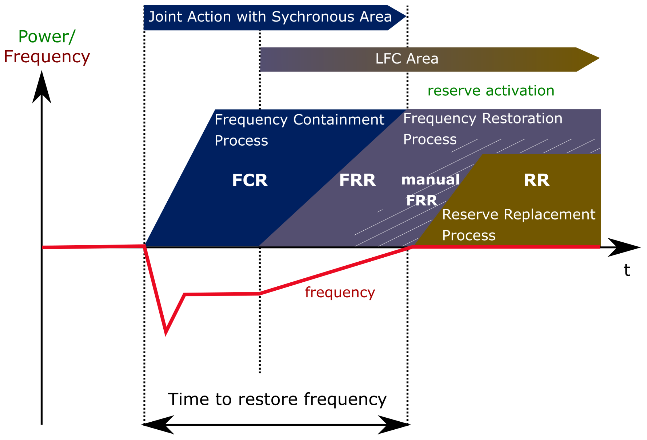
2. Load Frequency Control
- Frequency Containment Reserve (FCR)
- automatic Frequency Restoration Reserve (aFRR)
- manual Frequency Restoration Reserve (mFRR)
- Replacement Reserve (RR)
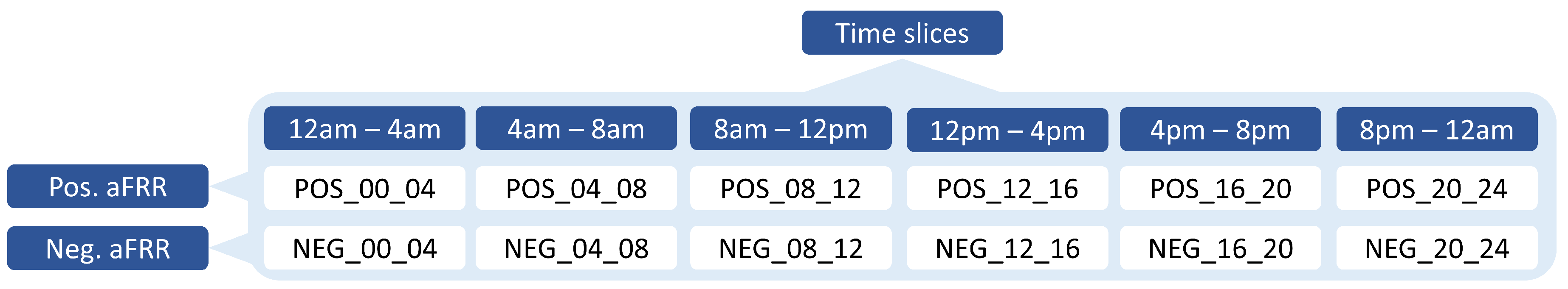
2.1. Frequency Restoration Reserve (FRR)
2.2. Modeling and Methods
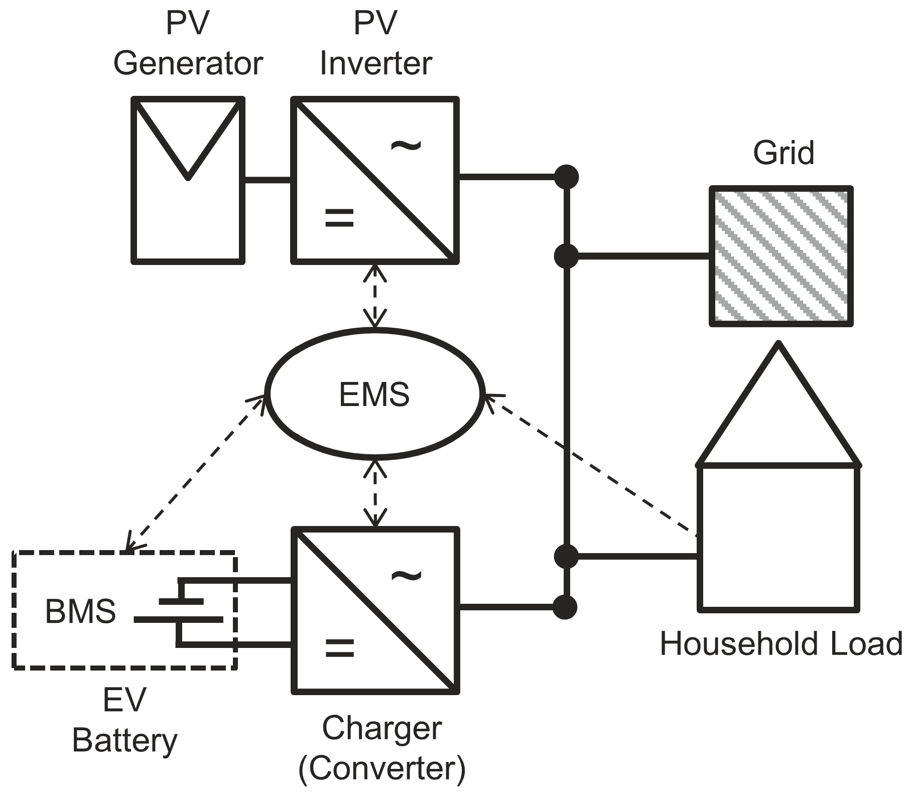
Model Setup and Components
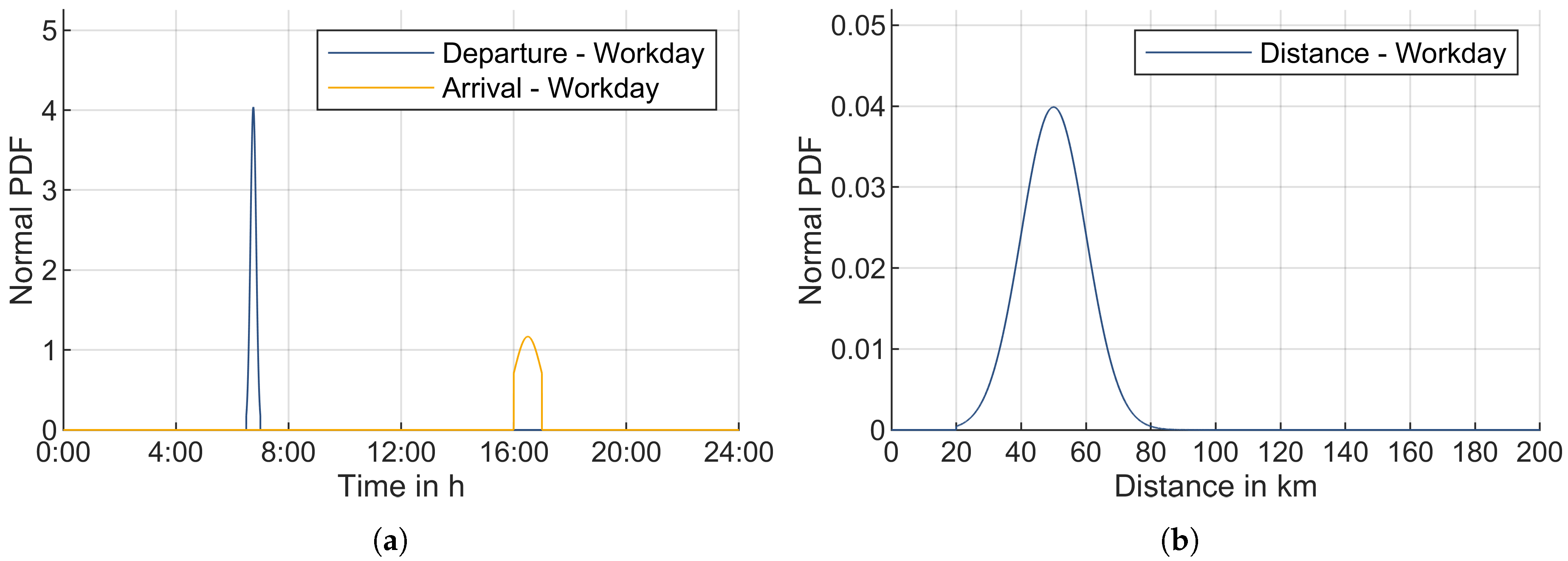
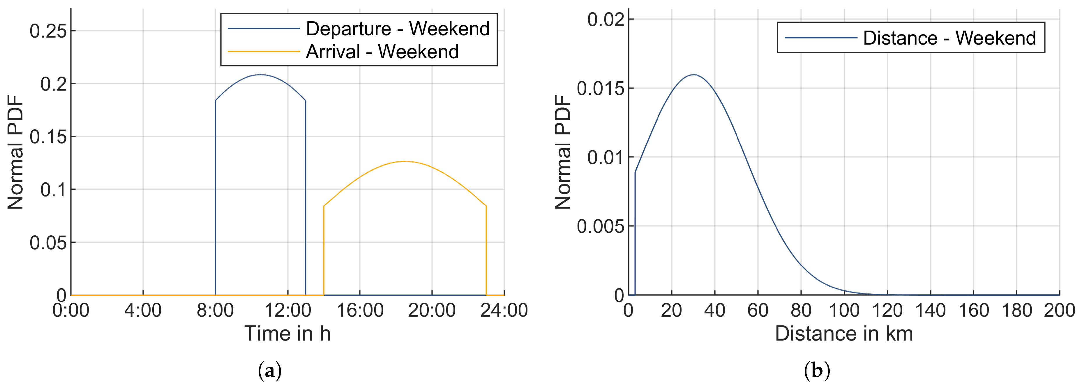
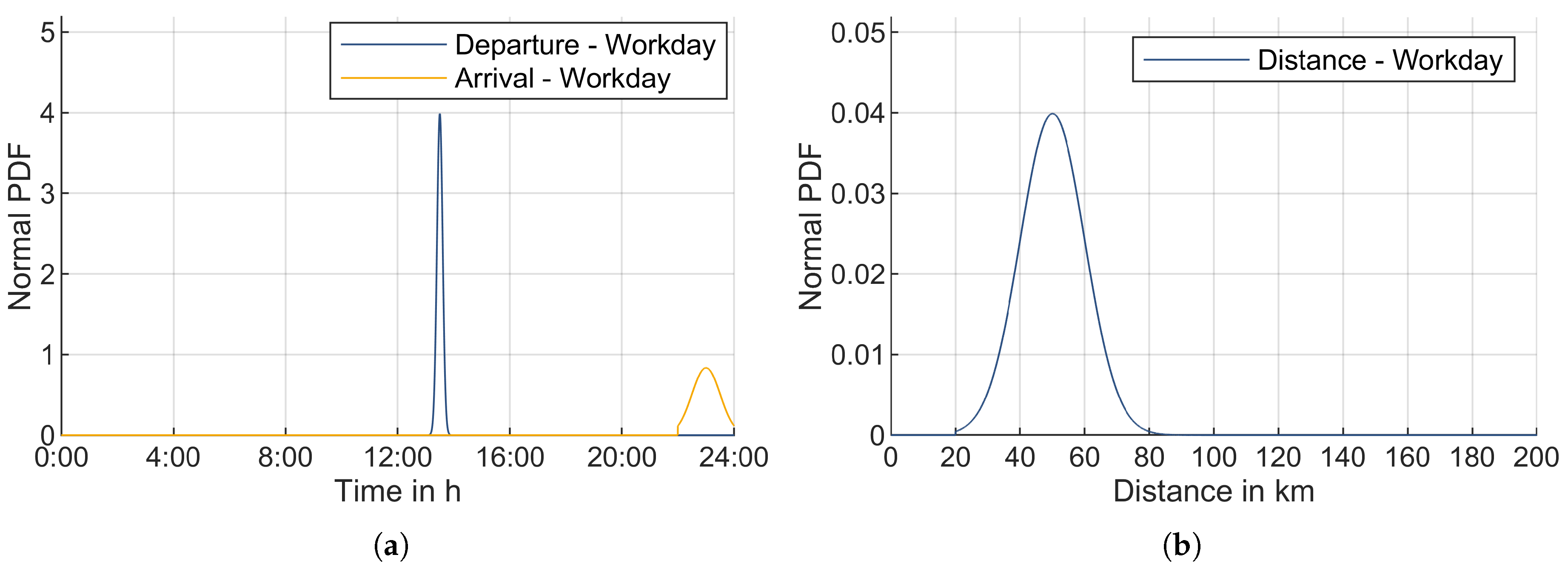
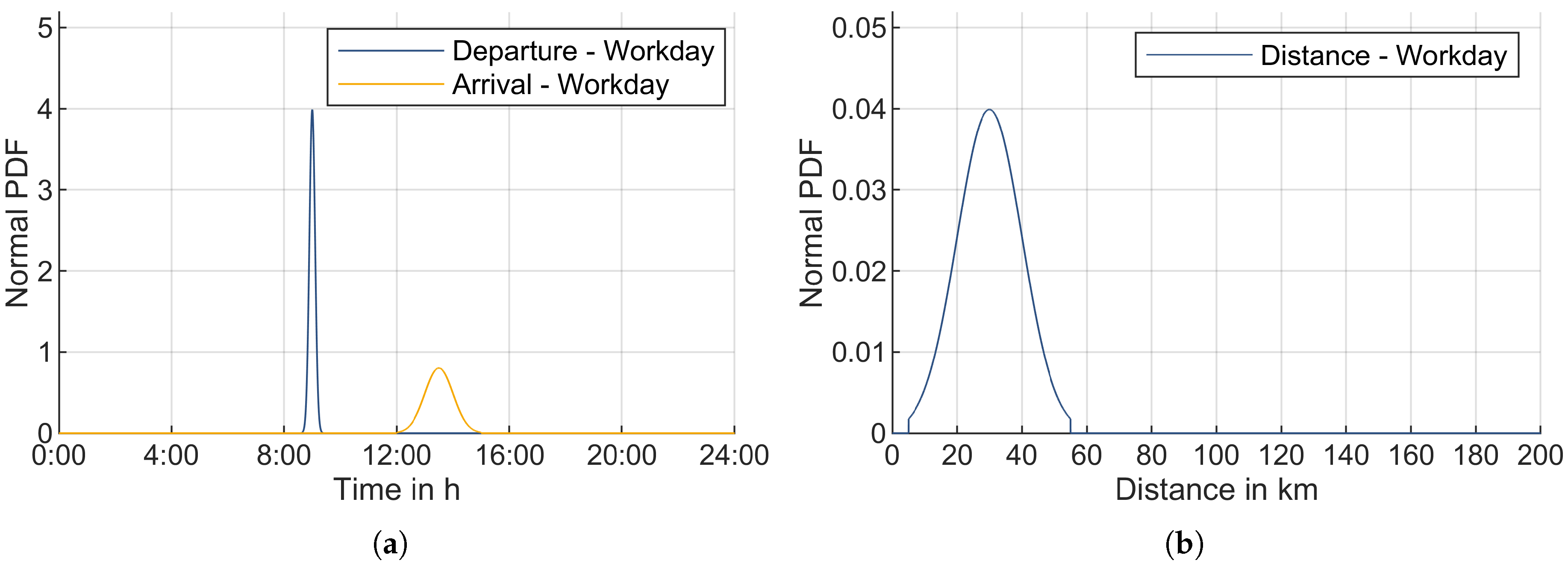
2.3. Mobility Profiles
2.4. Charging Strategies and Scenarios
- Reduction of electricity costs for the owner of the household and the EV
- Increase of self-consumption of electrical energy generated by the PV systems
- Increase of self-sufficiency of the household and of the workplace
- Reduction of calendar battery aging
- High availability of the EV for mobility
- Reduction of the power exchanged with the grid by household and workplace
Evaluation
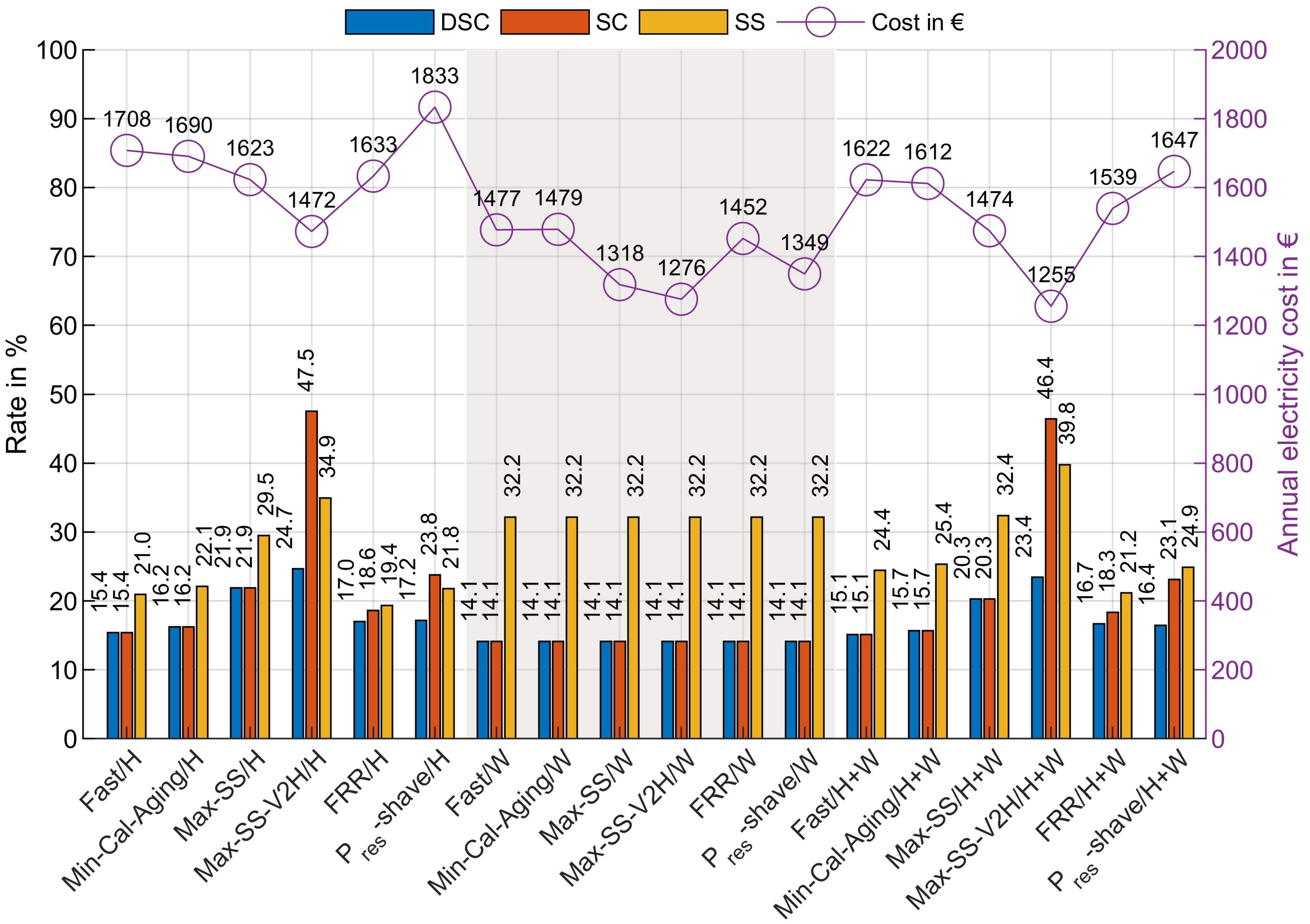
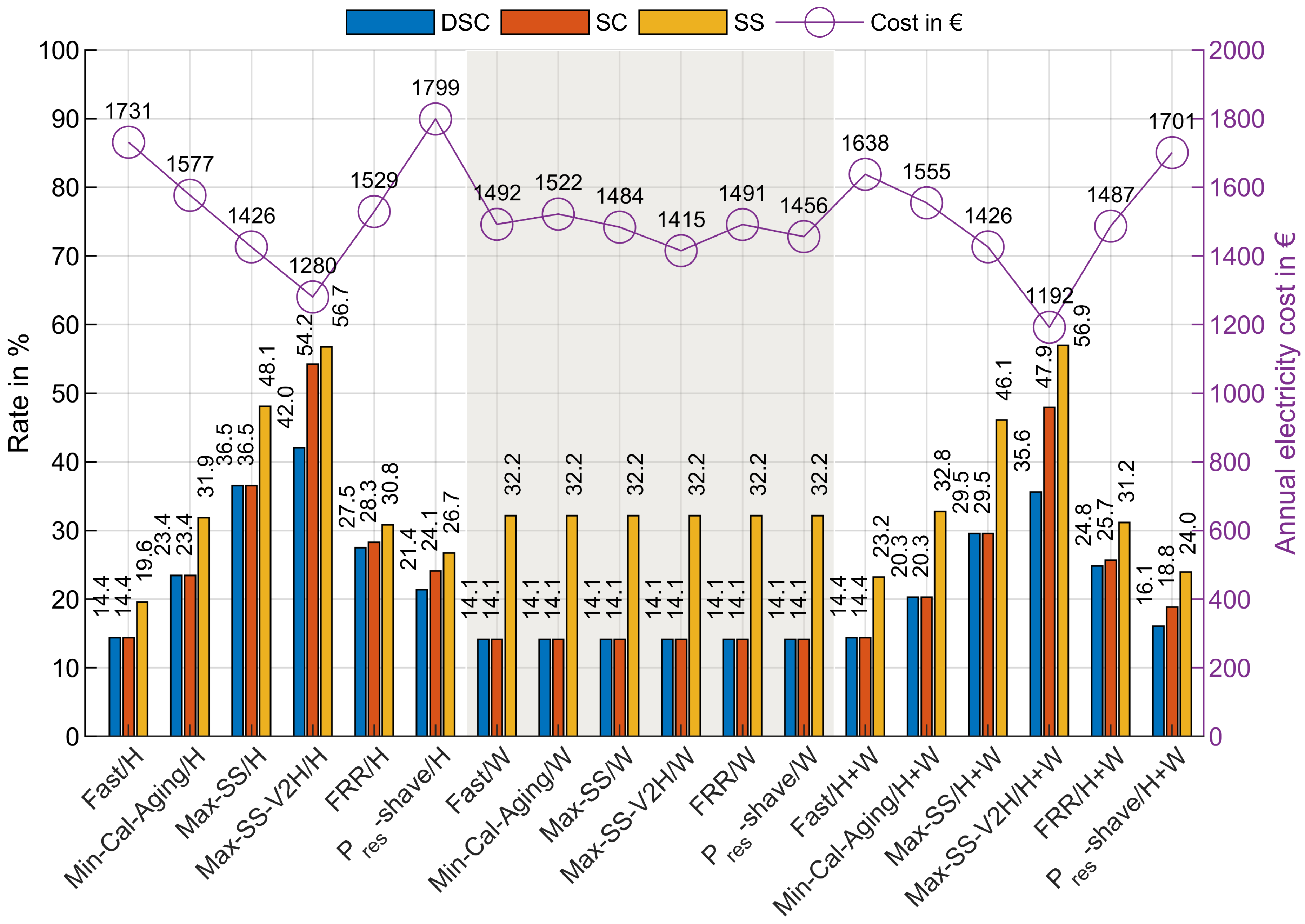
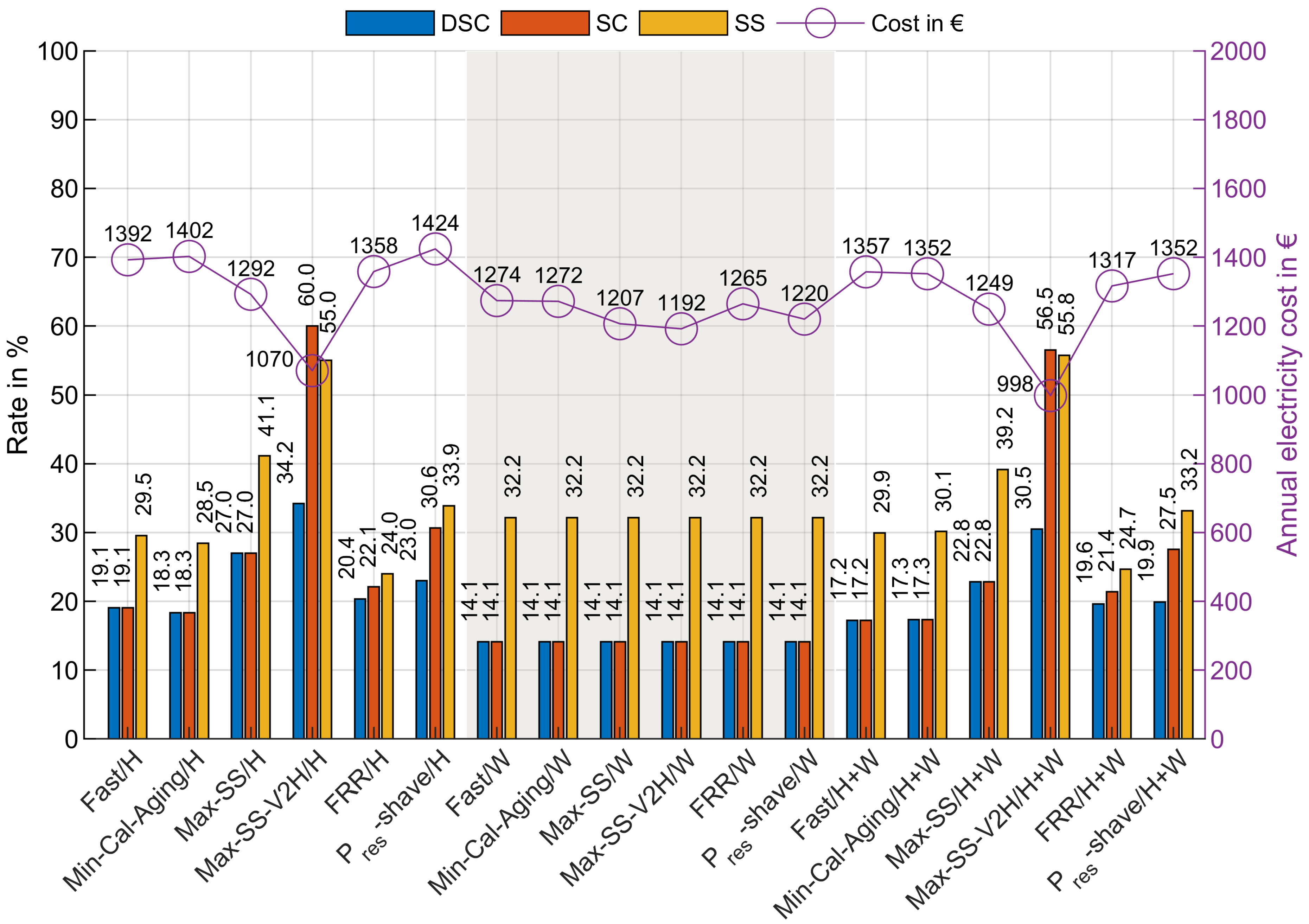
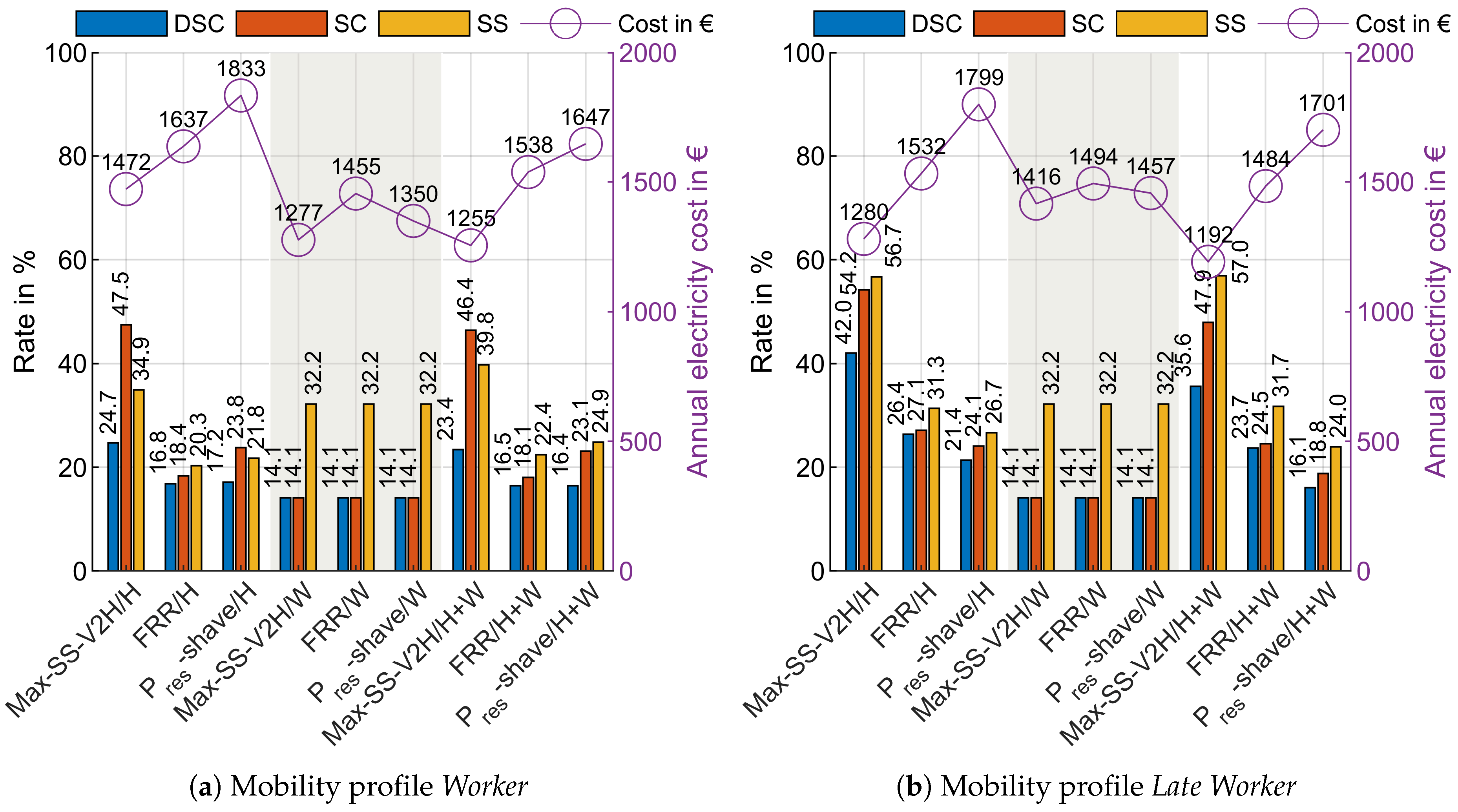
3. Results and Discussion
3.1. Workplace Charging Scenarios
3.2. Home Charging Scenarios
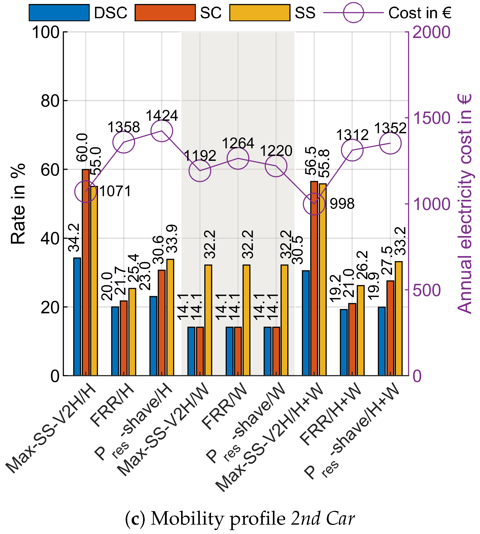
3.3. Home and Workplace Charging Scenarios
3.4. Fast Strategy
3.5. Min-Cal-Aging Strategy
3.6. Max-SS Strategy
3.7. Max-SS-V2H Strategy
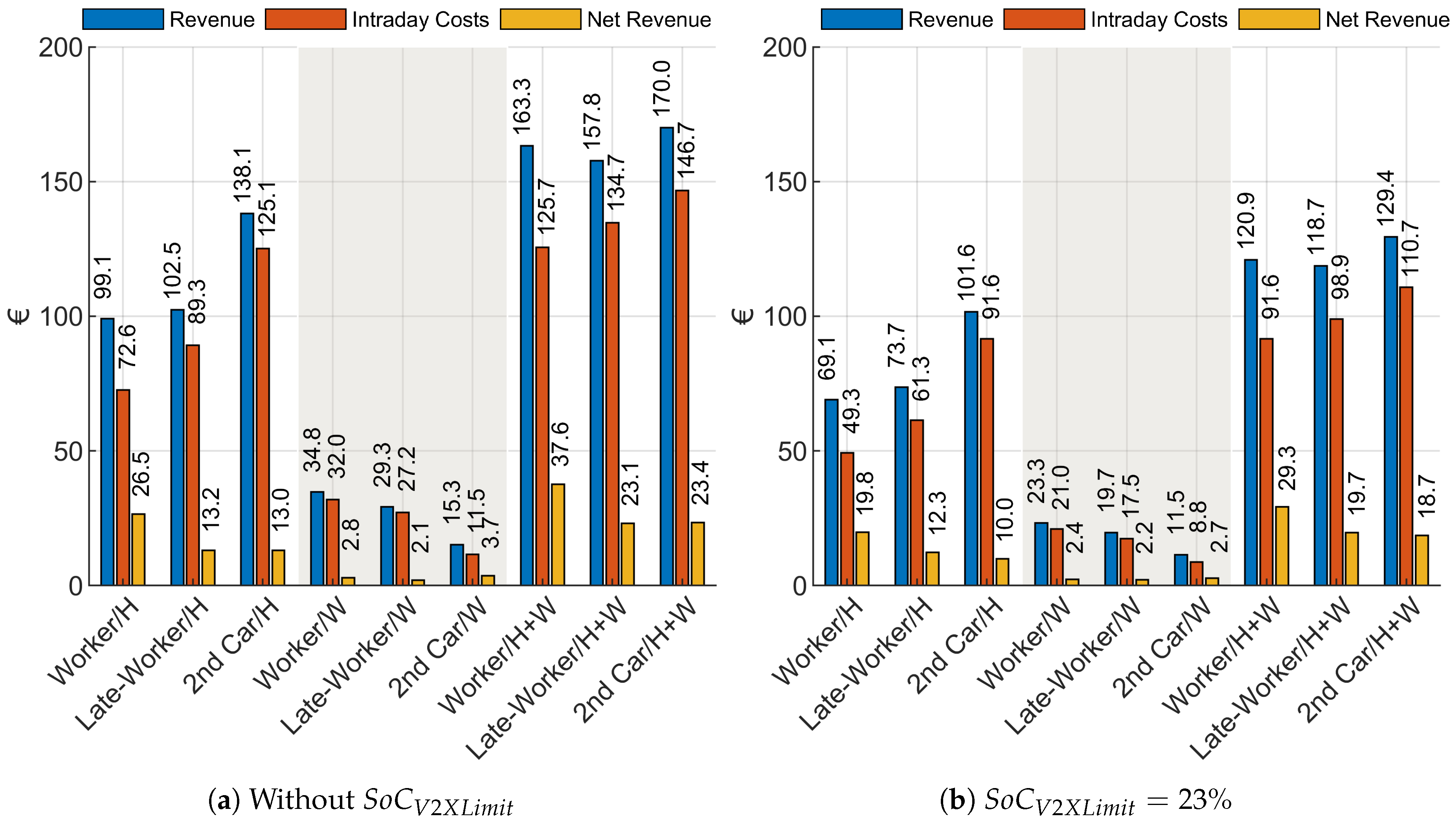
3.8. FRR Strategy
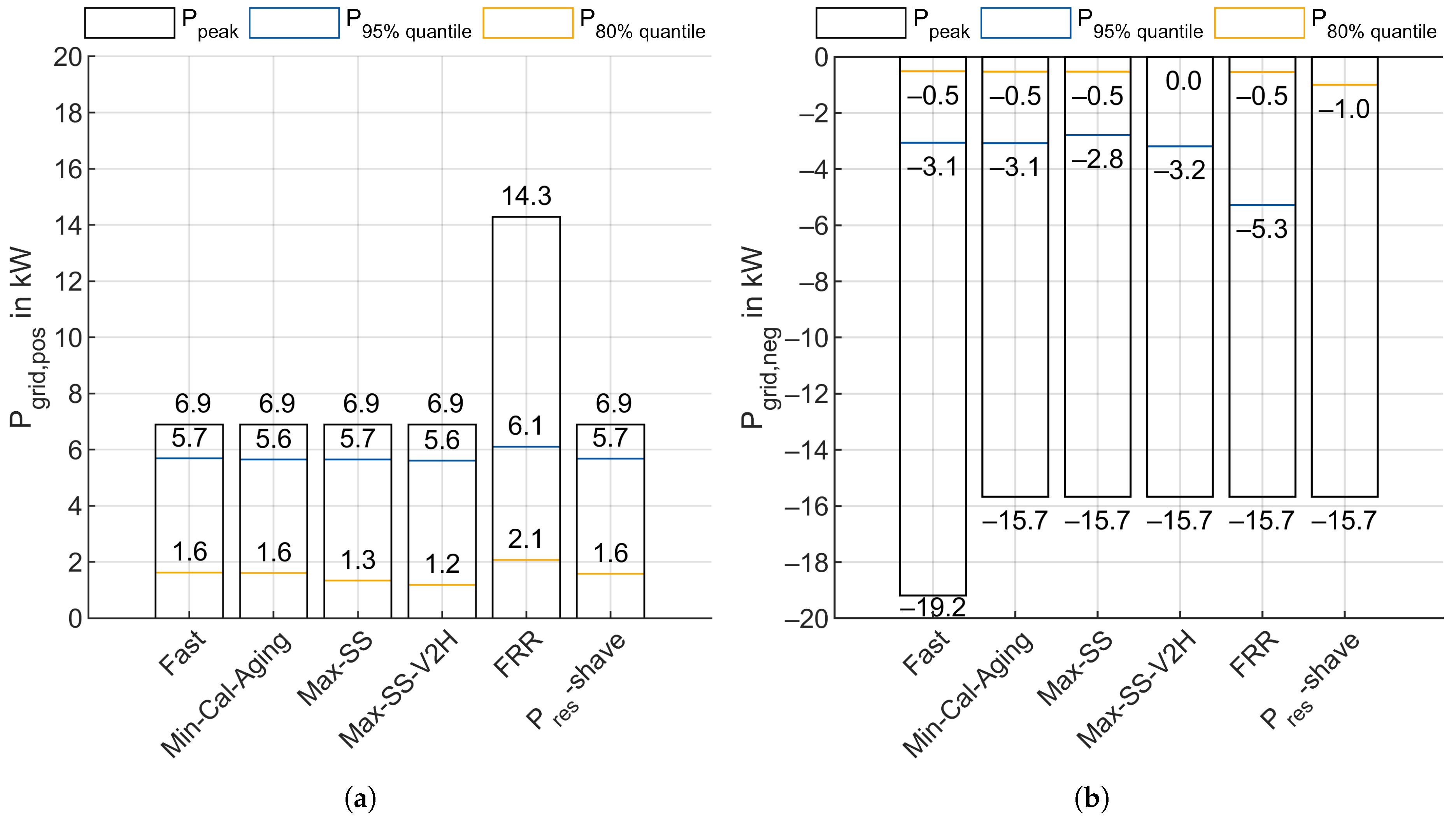
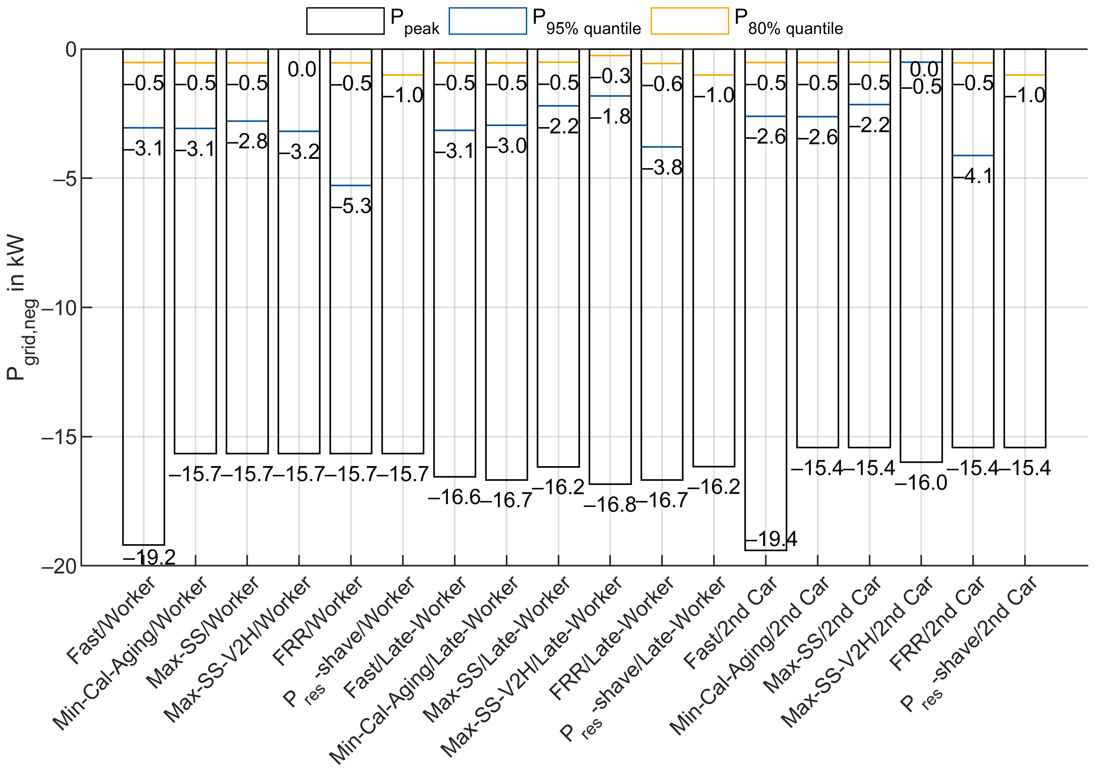
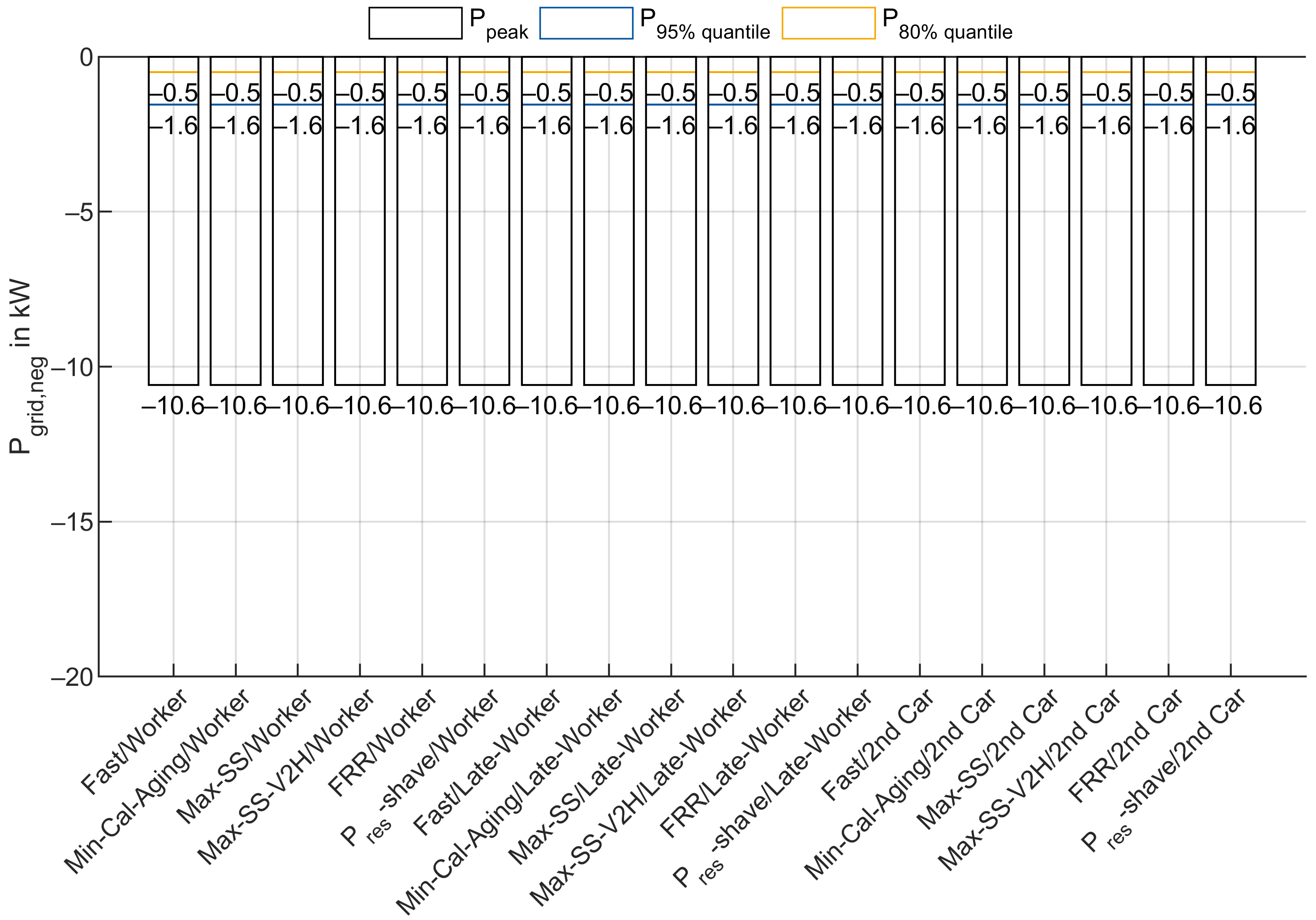
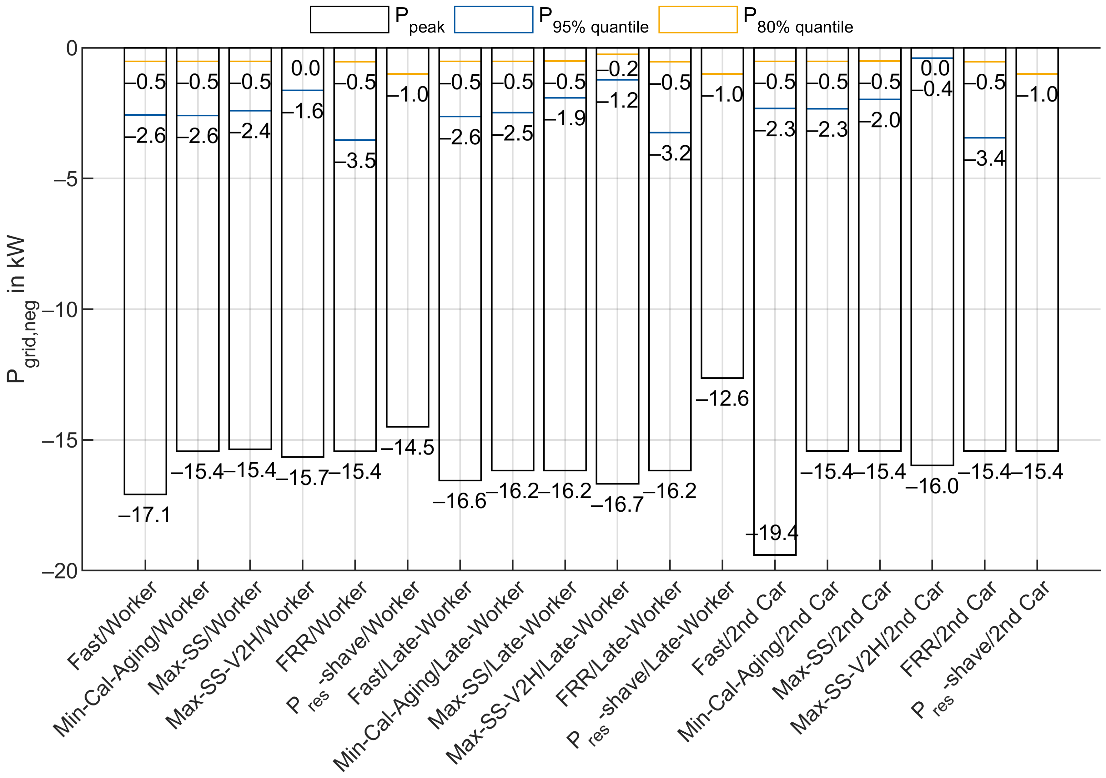
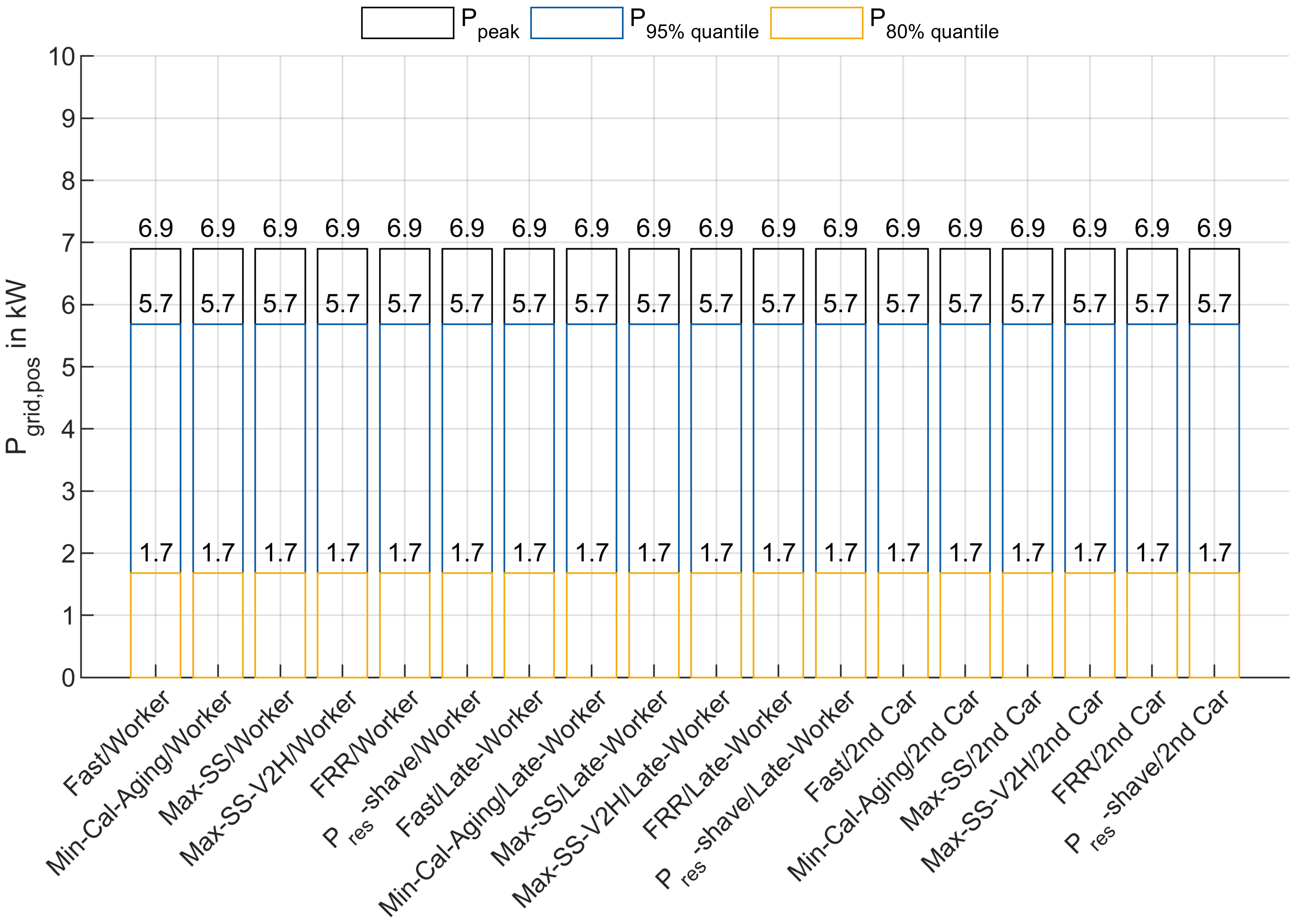
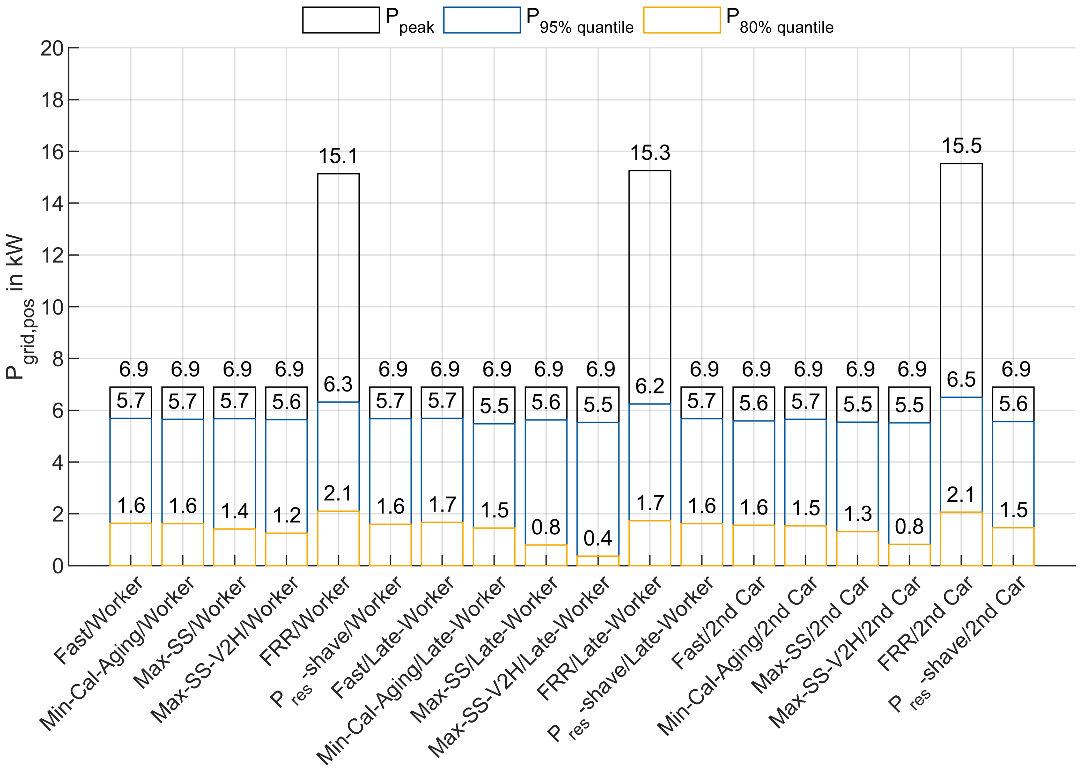
3.9. Strategy and the Power Exchanged with the Grid
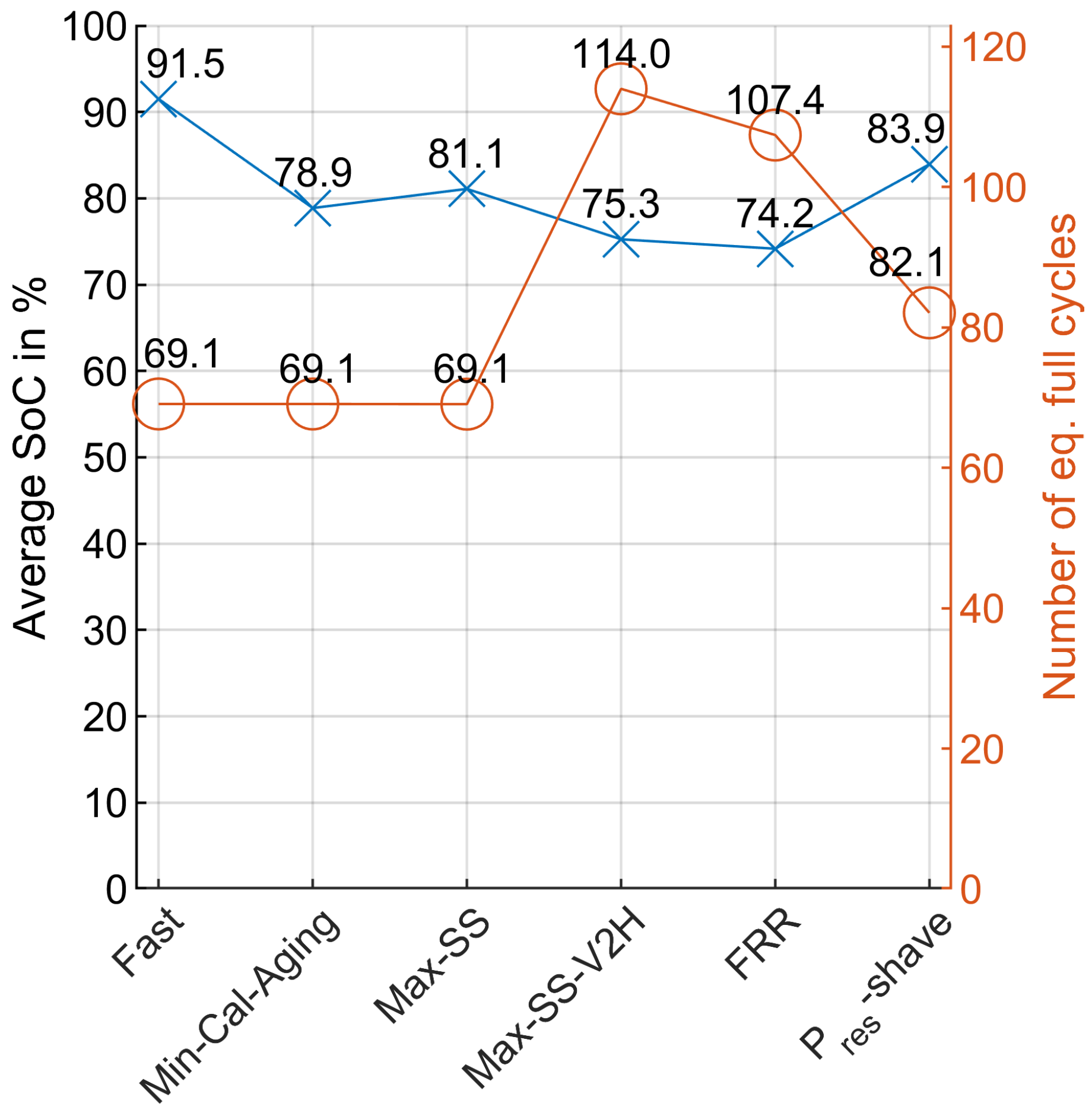
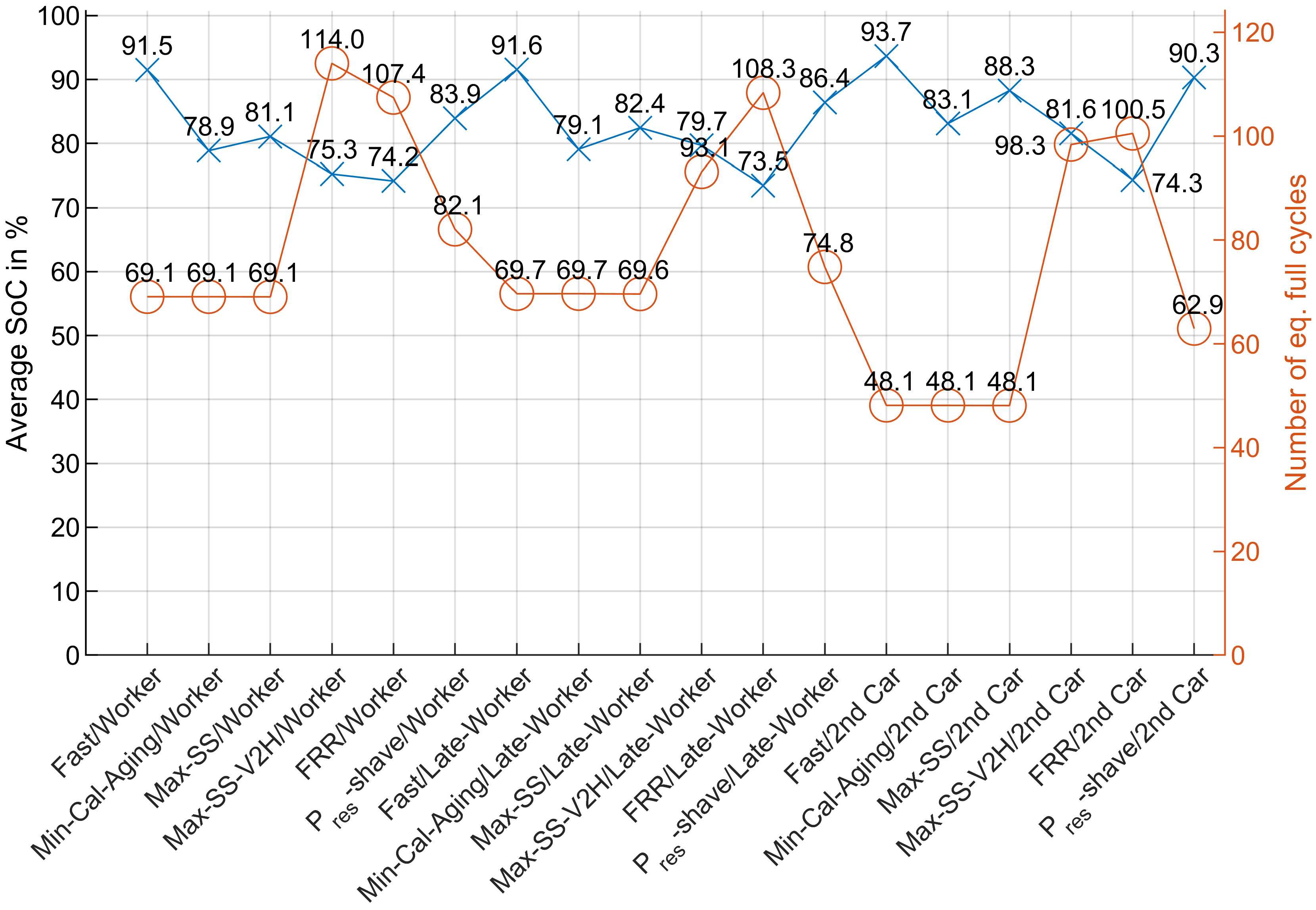
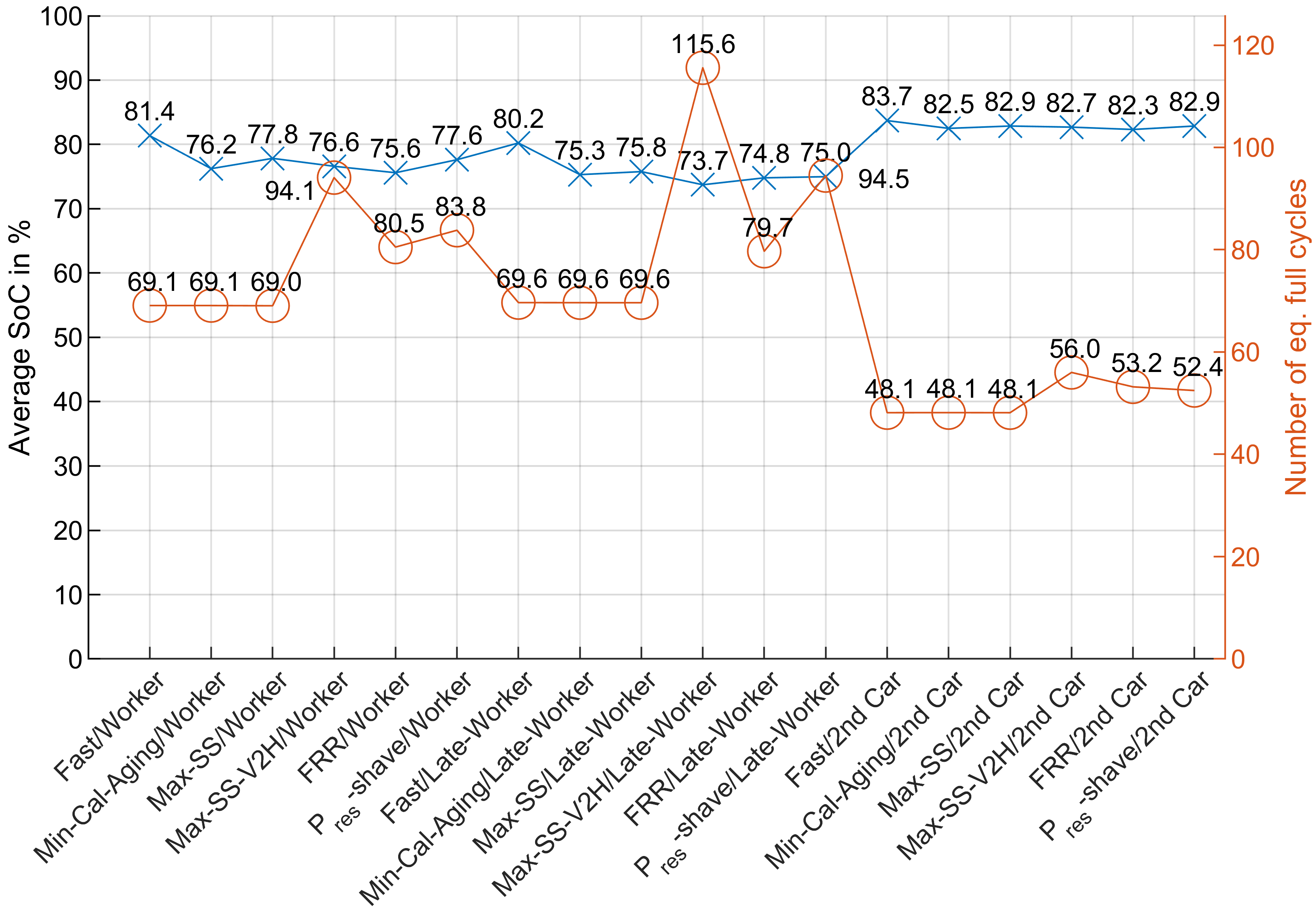
Average SoC and Number of Equivalent Full Cycles
4. Conclusions
Author Contributions
Funding
Conflicts of Interest
Abbreviations
| aFRR | Automatic Frequency Restoration Reserves |
| BMS | Battery Management System |
| BRP | Balance Responsible Party |
| DSC | Direct Self-Consumption |
| EEG | Renewable Energy Sources Act |
| EFC | Equivalent Full Cycle |
| EMS | Energy Management System |
| EV | Electric Vehicle |
| FCR | Frequency Containment Reserve |
| GHG | Greenhouse Gas |
| KPI | Key Performance Indicator |
| LFC | Load Frequency Control |
| mFRR | Manual Frequency Restoration Reserve |
| Probability Density Function | |
| PV | Photovoltaic |
| RR | Replacement Reserve |
| SC | Self-Consumption |
| SoC | State of Charge |
| SS | Self-Sufficiency |
| TSO | Transmission System Operator |
| V2X | Vehicle-to-X |
| V2G | Vehicle-to-Grid |
| V2H | Vehicle-to-Home |
Appendix A.
Appendix A.1. Mobility Profiles 2 and 3


Appendix A.2. Grid Power Exchange and Battery Stress


References
- Paris Agreement. United Nations Treaty Collection; United Nations: New York, NY, USA, 2016. [Google Scholar]
- Fraunhofer ISE Energy Chart. 2020. Available online: www.energy-charts.de (accessed on 14 April 2020).
- Dr. Harry Wirth | Fraunhofer ISE. Aktuelle Fakten zur Photovoltaik in Deutschland. 2020. Available online: www.ise.fraunhofer.de/content/dam/ise/de/documents/publications/studies/aktuelle-fakten-zur-photovoltaik-in-deutschland.pdf (accessed on 14 April 2020).
- Merkblatt Erneuerbare Energien- KfW-Programm Erneuerbare Energien “Speicher”. 25 May 2018. Available online: www.kfw.de/Download-Center/F%C3%B6rderprogramme-(Inlandsf%C3%B6rderung)/PDF-Dokumente/6000002700M275Speicher.pdf (accessed on 20 April 2020).
- Angenendt, G.; Zurmühlen, S.; Axelsen, H.; Sauer, D.U. Comparison of different operation strategies for PV battery home storage systems including forecast-based operation strategies. Appl. Energy 2018, 229, 884–899. [Google Scholar] [CrossRef]
- Schram, W.L.; Lampropoulos, I.; van Sark, W.G. Photovoltaic systems coupled with batteries that are optimally sized for household self-consumption: Assessment of peak shaving potential. Appl. Energy 2018, 223, 69–81. [Google Scholar] [CrossRef]
- Barzegkar-Ntovom, G.A.; Chatzigeorgiou, N.G.; Nousdilis, A.I.; Vomva, S.A.; Kryonidis, G.C.; Kontis, E.O.; Georghiou, G.E.; Christoforidis, G.C.; Papagiannis, G.K. Assessing the viability of Battery Energy Storage Systems coupled with Photovoltaics under a pure self-consumption scheme. Renew. Energy 2020, 152, 1302–1309. [Google Scholar] [CrossRef] [Green Version]
- Munkhammar, J.; Grahn, P.; Widén, J. Quantifying self-consumption of on-site photovoltaic power generation in households with electric vehicle home charging. Sol. Energy 2013, 97, 208–216. [Google Scholar] [CrossRef]
- Englberger, S.; Hesse, H.; Kucevic, D.; Jossen, A. A Techno-Economic Analysis of Vehicle-to-Building: Battery Degradation and Efficiency Analysis in the Context of Coordinated Electric Vehicle Charging. Energies 2019, 12, 955. [Google Scholar] [CrossRef] [Green Version]
- Chakravorty, D.; Chaudhuri, B.; Hui, S.Y.R. Rapid Frequency Response From Smart Loads in Great Britain Power System. IEEE Trans. Smart Grid 2017, 8, 2160–2169. [Google Scholar] [CrossRef] [Green Version]
- Litjens, G.; Worrell, E.; van Sark, W. Economic benefits of combining self-consumption enhancement with frequency restoration reserves provision by photovoltaic-battery systems. Appl. Energy 2018, 223, 172–187. [Google Scholar] [CrossRef]
- Münderlein, J.; Steinhoff, M.; Zurmühlen, S.; Sauer, D.U. Analysis and evaluation of operations strategies based on a large scale 5 MW and 5 MWh battery storage system. J. Energy Storage 2019, 24, 100778. [Google Scholar] [CrossRef]
- Statkraft Direktvermarkung MRL Wind Power. 2020. Available online: www.statkraftdirektvermarktung.de/pioniergeist/minutenreserveleistung-wind (accessed on 14 April 2020).
- Next Kraftwerke VPP. Available online: www.next-kraftwerke.com/vpp/virtual-power-plant (accessed on 14 April 2020).
- Tennet. End Report FCR Pilot—FCR Delivery with Aggregated Assets; TenneT TSO B.V.: Arnhem, The Netherlands, 2018. [Google Scholar]
- Bach Andersen, P.; Hashemi Toghroljerdi, S.; Meier Sørensen, T.; Christensen, B.; Christian Morell Lodberg Høj, J.; Zecchino, A. The Parker Project; Technical University of Denmark: Lyngby, Denmark, 2019. [Google Scholar]
- Olk, C.; Sauer, D.U.; Merten, M. Bidding strategy for a battery storage in the German secondary balancing power market. J. Energy Storage 2019, 21, 787–800. [Google Scholar] [CrossRef]
- Angenendt, G.; Merten, M.; Zurmühlen, S.; Sauer, D.U. Evaluation of the effects of frequency restoration reserves market participation with photovoltaic battery energy storage systems and power-to-heat coupling. Appl. Energy 2020, 260, 114186. [Google Scholar] [CrossRef]
- Jargstorf, J.; Wickert, M. Offer of secondary reserve with a pool of electric vehicles on the German market. Energy Policy 2013, 62, 185–195. [Google Scholar] [CrossRef]
- 50Hertz Transmission GmbH, Amprion GmbH, TenneT TSO GmbH, TransnetBW GmbH. regelleistung.net. Available online: www.regelleistung.net/ext/tender/remark/news/433 (accessed on 8 April 2020).
- KU Leuven Energy Institute. EIectricity_Market_Factsheet; KU Leuven: Leuven, Belgium, 2015; Available online: https://set.kuleuven.be/ei/factsheets (accessed on 20 April 2020).
- EPEX Group. Available online: www.epexspot.com/en/tradingproducts-intraday-trading (accessed on 8 April 2020).
- ENTSO-E. Supporting Paper for the Load-Frequency Control and Reserves Network Code; ENTSO-E: Brussels, Belgium, 28 June 2013. [Google Scholar]
- European Comission. COMMISSION REGULATION (EU) 2017/1485—Of 2 August 2017—Establishing a Guideline on Electricity Transmission System Operation; European Comission: Brussels, Belgium, 2017. [Google Scholar]
- 50Hertz Transmission GmbH, Amprion GmbH, TenneT TSO GmbH, TransnetBW GmbH. regelleistung.net. Available online: www.regelleistung.net/ext/static/prl (accessed on 8 April 2020).
- Merten, M.; Olk, C.; Schoeneberger, I.; Sauer, D.U. Bidding strategy for battery storage systems in the secondary control reserve market. Appl. Energy 2020, 268, 114951. [Google Scholar] [CrossRef]
- Merten, M.; Rücker, F.; Schoeneberger, I.; Sauer, D.U. Automatic Frequency Restoration Reserve Market Prediction: Methodology and Comparison of Various Approaches. Appl. Energy 2020, 268, 114978. [Google Scholar] [CrossRef]
- Magnor, D.; Gerschler, J.B.; Ecker, M.; Merk, P.; Sauer, D.U. Concept of a Battery Aging Model for Lithium-Ion Batteries Considering the Lifetime Dependency on the Operation Strategy. In Proceedings of the 24th European Photovoltaic Solar Energy Conference, Hamburg, Germany, 21–25 September 2009; pp. 3128–3134. [Google Scholar] [CrossRef]
- Magnor, D. Globale Optimierung netzgekoppelter PV-Batteriesysteme unter besonderer Berücksichtigung der Batteriealterung; RWTH Aachen: Aachen, Germany, 2017. [Google Scholar]
- Figgener, J.; Haberschusz, D.; Kairies, K.P.; Wessels, O.; Tepe, B.; Sauer, D.-U. Wissenschaftliches Mess- und Evaluierungsprogramm Solarstromspeicher 2.0 [Scientific Measuring and Evaluation Program for Photovoltaic Battery Systems]: Jahresbericht 2018; ISEA Institute for Power Electronics and Electrical Drives, RWTH Aachen: Aachen, Germany, 2018. [Google Scholar]
- European Comission. Teil III: Anleitung für die Ausführung von Normungsaufträgen. In Leitfaden zur europäischen Normung als Unterstützung für legislative und politische Maßnahmen der Union; European Comission: Brussels, Belgium, 2015. [Google Scholar]
- Sauer, D.-U. Untersuchungen zum Einsatz und Entwicklung von Simulationsmodellen für die Auslegung von Photovoltaik-Systemen. Diploma Thesis, TH Darmstadt, Darmstadt, Germany, 1994. [Google Scholar]
- Behrens, K. Horizon at Station Lindenberg. 2007. Available online: https://0-doi-org.brum.beds.ac.uk/10.1594/PANGAEA.669521 (accessed on 20 April 2020).
- Bost, M.; Hirschl, B.; Aretz, A. Effekte von Eigenverbrauch und Netzparität bei der Photovoltaik—Langfassung; Institut für ökologische Wirtschaftsforschung (IÖW) GmbH, gemeinnützig: Berlin, Germany, 2011. [Google Scholar]
- Daimler, AG. Available online: https://media.daimler.com/marsMediaSite/ko/en/9920260 (accessed on 20 April 2020).
- Infas Institut für angewandte Sozialwissenschaft GmbH. Mobilität in Deutschland 2017—Ergebnisbericht; BMVI: Berlin, Germany, 2017. [Google Scholar]
- Schmalstieg, J.; Käbitz, S.; Ecker, M.; Sauer, D.U. A holistic aging model for Li(NiMnCo)O2 based 18650 lithium-ion batteries. J. Power Sources 2014, 257, 325–334. [Google Scholar] [CrossRef]
- Kost, C.; Schlegl, T.; Jülch, V.; Nguyen, H.T.; Schlegl, T. Stromgestehungskosten Erneuerbare Energien; Fraunhofer ISE: Freiburg, Germany, March 2018. [Google Scholar]
- Bundesnetzagentur; Bundeskartellamt. Monitoringbericht 2019; Bundesnetzagentur: Bonn, Germany, 2019. [Google Scholar]
- gridX GmbH. Available online: www.gridx.de/produkt/gridbox (accessed on 13 April 2019).
- Photovoltaikforum.com. Regelleistungsmodell von Caterva: “Für jedes Kilowatt Regelleistung 150 bis 160 Euro im Jahr”. Available online: www.photovoltaikforum.com/magazin/praxis/regelleistungsmodell-von-caterva-fuer-jedes-kilowatt-regelleistung-150-bis-160-euro-im-jahr-4765/ (accessed on 13 April 2019).


| Electric Vehicle | PV System | Household | |||
|---|---|---|---|---|---|
| Persons | 4 | ||||
| 38 | |||||
| (south) | |||||
| SoC Range | 3.2–95.3% | ||||
| Battery layout | 93S1P | 9734 /a | |||
| Ah | |||||
| Annual Driving Distance | Worker: 14,743 km | ||||
| Late-Worker: 14,924 km | |||||
| 2nd Car: 10,211 km | |||||
| 10 | |||||
| Mobility Profile | Day | Parameter | Lower Limit | Upper Limit | ||
|---|---|---|---|---|---|---|
| Worker | Workday | Departure | 6:45 h | 6:30 h | 7:00 h | |
| Arrival | 16:30 h | 16:00 h | 17:00 h | |||
| Distance | 50 | 10 | 20 | 110 | ||
| Late Worker | Workday | Departure | 13:30 h | 13:00 h | 14:00 h | |
| Arrival | 23:00 h | 22:00 h | 24:00 h | |||
| Distance | 50 | 10 | 20 | 110 | ||
| 2nd Car | Workday | Departure | 9:00 h | 8:30 h | 10:30 h | |
| Arrival | 13:30 h | 12:00 h | 15:00 h | |||
| Distance | 30 | 10 | 5 | 55 | ||
| Worker, | Weekend | Departure | 10:30 h | 5 | 8:00 h | 13:00 h |
| Late-Worker, | Arrival | 18:30 | 5 | 14:00 h | 23:00 h | |
| 2nd Car | Distance | 30 | 25 | 3 | 180 |
| Charging Strategy | Charging Location | Mobility Profile | |
|---|---|---|---|
| Fast | Home (H) | Worker | not set |
| Min-Cal-Aging | Workplace (W) | Late Worker | 23% |
| Max-SS | Home & Workplace (H + W) | 2nd Car | |
| Max-SS-V2H | |||
| FRR | |||
| -shave |
| Charging Strategy | Information |
|---|---|
| Fast | None |
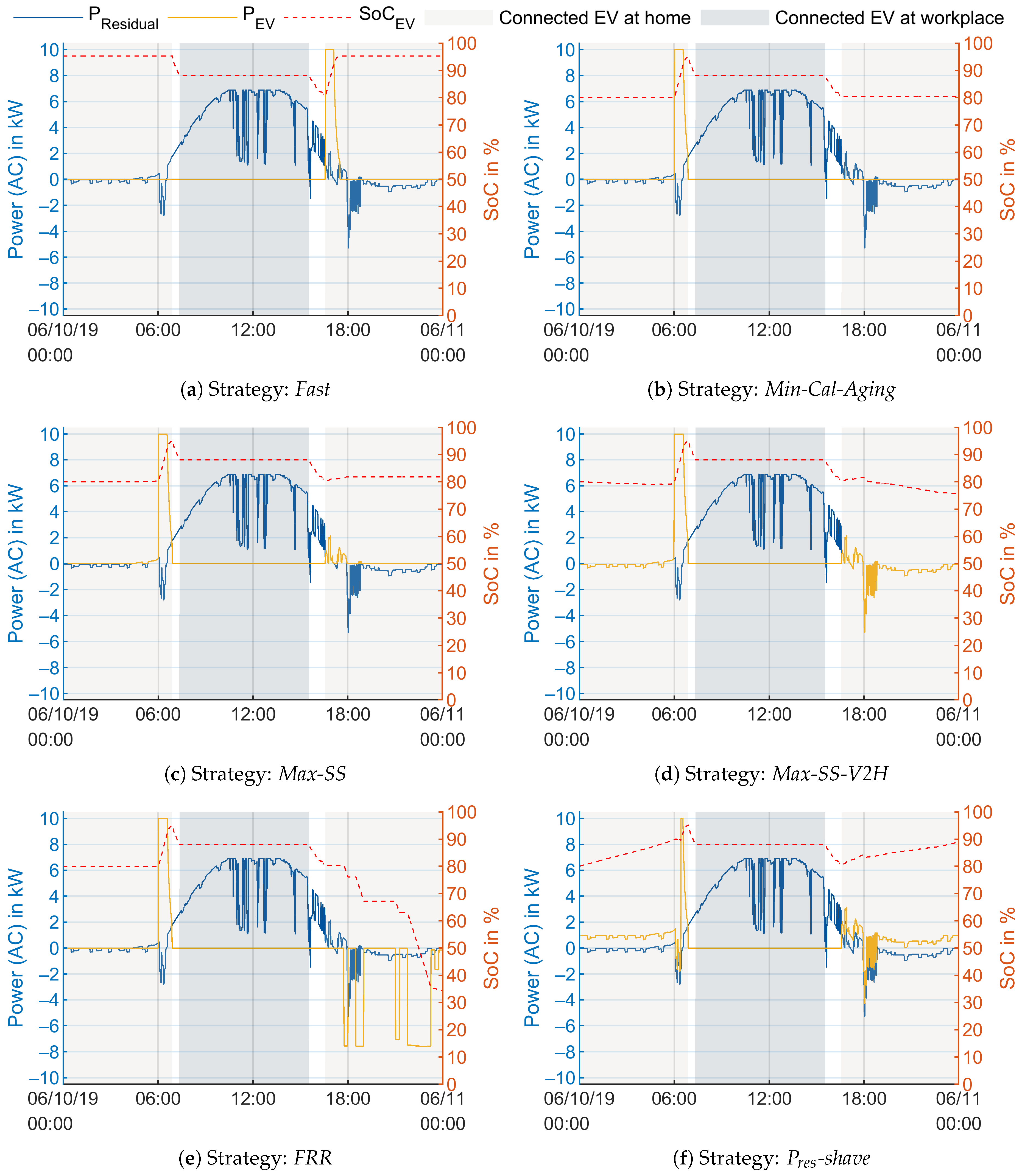
| Upon arrival, the EV is charged with the maximum charging power (10 kW) until it is fully charged. This strategy maximizes the availability of the EV for the user (Objective E). See the functionality of the strategy in Figure 7a. | |
| Min-Cal-Aging | Time of departure of EV |
| This strategy aims to reduce the average SoC of the EV battery (Objective D). For Li-Ion batteries with an NMC chemistry an elevated SoC leads to accelerated calendar aging [37]. The charge process of the EV is delayed in order to reduce average SoC. The EMS calculates the latest point in time to start charging the EV with maximal power in order to fully charge the EV by the time of departure. See the functionality of the strategy in Figure 7b. | |
| Max-SS | Time of departure of EV, Residual Load () |
| This strategy charges the EV when positive residual power is available. Then the charging power is set to the value of . As a result the EV is charged with electrical energy generated by the PV system. This strategy aims to increase the self-consumption (SC) and self-sufficiency (SS) of the household (Objectives A, B, and C). If the residual energy is not sufficient to fully charge the EV before departure, the EV is charged with maximum power (10 ) before departure. See the functionality of the strategy in Figure 7c. | |
| Max-SS-V2H | Time of departure of EV, residual load, |
| This strategy is an extension of strategy Max-SS. In addition to the functionality of Max-SS, the EV discharges with negative residual power when load exceeds PV generation. This strategy aims to increase the self-consumption and self-sufficiency of the household using V2H (Objectives A, B, and C). See the functionality of the strategy in Figure 7d. | |
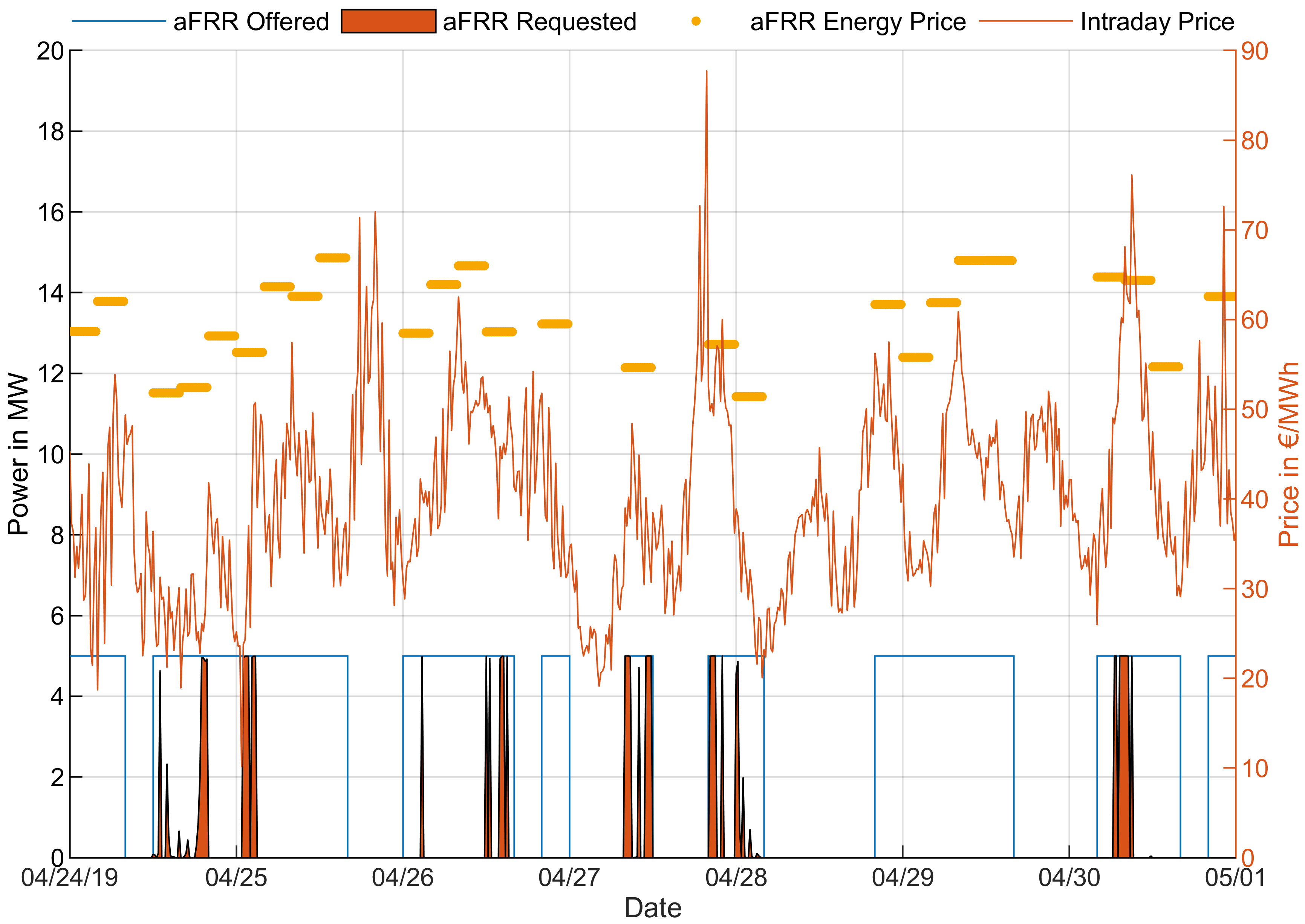
| FRR | Time of departure of EV, residual load, , aFRR request |
| The EV is integrated into a pool of units that provide positive aFRR. The aggregator of the pool forecasts the power capacity of the pool in order to bid on the aFRR market. For this study we use a time-series of the awarded aFRR participation and the aFRR requests for the time period 30 October 2018–30 July 2019 (9 Months). See Section 2.1 for further details and Figure 3 for a snapshot of the time series. Due to the 4 hour criterion, the power that can be offered by the EV is calculated at the time of plug-in at the charging station. It is calculated as follows, | |
| -shave | Time of departure of EV, residual load, , |
| The strategy aims to keep the absolute value of the residual load of the household under limit in order to reduce the power exchanged with the grid (Objective F). In this study . The EV charges with when and discharges to the home with when . As no forecast algorithms are used, the peak production might not be shaved due to the fact that the EV is already fully charged when it occurs. Moreover, due to the lack of forecast, a peak for the charge of the EV before departure may occur as, starting at the latest possible point in time, the remaining energy is charged with maximum power (10). See the functionality of the strategy in Figure 7f. | |
© 2020 by the authors. Licensee MDPI, Basel, Switzerland. This article is an open access article distributed under the terms and conditions of the Creative Commons Attribution (CC BY) license (http://creativecommons.org/licenses/by/4.0/).
Share and Cite
Rücker, F.; Merten, M.; Gong, J.; Villafáfila-Robles, R.; Schoeneberger, I.; Sauer, D.U. Evaluation of the Effects of Smart Charging Strategies and Frequency Restoration Reserves Market Participation of an Electric Vehicle. Energies 2020, 13, 3112. https://0-doi-org.brum.beds.ac.uk/10.3390/en13123112
Rücker F, Merten M, Gong J, Villafáfila-Robles R, Schoeneberger I, Sauer DU. Evaluation of the Effects of Smart Charging Strategies and Frequency Restoration Reserves Market Participation of an Electric Vehicle. Energies. 2020; 13(12):3112. https://0-doi-org.brum.beds.ac.uk/10.3390/en13123112
Chicago/Turabian StyleRücker, Fabian, Michael Merten, Jingyu Gong, Roberto Villafáfila-Robles, Ilka Schoeneberger, and Dirk Uwe Sauer. 2020. "Evaluation of the Effects of Smart Charging Strategies and Frequency Restoration Reserves Market Participation of an Electric Vehicle" Energies 13, no. 12: 3112. https://0-doi-org.brum.beds.ac.uk/10.3390/en13123112