Triple Solutions of Carreau Thin Film Flow with Thermocapillarity and Injection on an Unsteady Stretching Sheet

Abstract

Thin films and coatings which have a high demand in a variety of industries—such as manufacturing, optics, and photonics—need regular improvement to sustain industrial productivity. Thus, the present work examined the problem of the Carreau thin film flow and heat transfer with the influence of thermocapillarity over an unsteady stretching sheet, numerically. The sheet is permeable, and there is an injection effect at the surface of the stretching sheet. The similarity transformation reduced the partial differential equations into a system of ordinary differential equations which is then solved numerically by the MATLAB boundary value problem solver bvp4c. The more substantial effect of injection was found to be the reduction of the film thickness at the free surface and development of a better rate of convective heat transfer. However, the increment in the thermocapillarity number thickens the film, reduces the drag force, and weakens the rate of heat transfer past the stretching sheet. The triple solutions are identified when the governing parameters vary, but two of the solutions gave negative film thickness. Detecting solutions with the most negative film thickness is essential because it implies the interruption in the laminar flow over the stretching sheet, which then affects the thin film growing process.

1. Introduction

The discovery of the boundary layer by Prandtl [1] remarked the highest achievement in the development of fluid mechanics and created a proper basis to understand the dynamics of the real fluid. The Prandtl boundary layer is found in a wide range of aerodynamics and engineering applications. The boundary layer idea then evolved into the theoretical works on the boundary layer flow over a stretching surface which was contributed by the following literature: Sakiadis [2,3], Crane [4], and Carragher and Crane [5]. These works were highly appreciated due to its significance in the extrusion process. As time progressed, the boundary layer flow has been probed under various circumstances to improve the quality of the extrusion process, and hence many works have been reported accordingly (see [6,7,8,9,10,11,12,13,14,15,16,17,18,19]). Cast film extrusion is an emerging industrial process that produces cast films which are widely used for food and textiles packaging and coating substrates in the extrusion coating process [20]. The demand for this process is still high, and research activities are conducted so that it can be improved from time to time. The theoretical work in thin film flow was started by Wang [21] by investigating the behavior of thin liquid film flow past an impermeable stretching surface and it was found that the similarity solutions were absent when the value of the unsteadiness parameter $\left(S\right)$ falls within the range of $S>2$. Usha and Sridharan [22] reexamined the work of [21] by considering the asymmetric flow and justified that the similarity solutions become unavailable when the value of the unsteadiness parameter fell within the range of $S>4$. Shortly thereafter, the subject of non-Newtonian fluid captured the attention of the researchers in the thin film flow since non-Newtonian fluid such as paint also used in the extrusion coating process. Thus, the problem of thin film flow towards an unsteady stretching sheet in a generalized non-Newtonian fluid was solved by Andersson et al. [23] and concluded that at a higher value of the unsteadiness parameter, the impact of the power-law index is more significant. The researchers then realized that the heat transfer aspect is also equally important as the fluid flow characteristics in a thin film flow so that the complications in the design of various heat exchangers and chemical processing equipment can be surmounted. Andersson et al. [24] came forward to investigate the heat transfer features in a thin film flow past an unsteady stretching surface and discovered that, at low Prandtl numbers $\left(\mathrm{Pr}<1\right),$ the effect of the unsteadiness parameter on the rate of heat transfer is highly significant. Chen [25] also was interested in studying the heat transfer characteristics in the thin film flow and hence revisited the work of [23] to examine the heat transfer feature in the power-law model considered in [23]. On the other hand, Wang [26] attempted to solve the thin film problem in [24] by using a different form of similarity transformation and generated the analytic solutions via the homotopy analysis method (HAM). The work of [26] proved that the analytic method also could be employed in the theoretical investigation of the thin film flow mechanism past a stretching sheet. After that, the thin film flow and heat transfer past an unsteady stretching sheet were investigated under various settings, for instance, see [27,28,29,30,31,32].

Thermocapillarity is a physical effect which formed through the thermally induced surface-tension gradients over a fluid–fluid interface [33]. Researchers then developed this effect in the thin film flow as the surface-tension gradients able to produce interfacial flow which can be found in the continuous casting process. The thermocapillarity effect seemed to be significant in crystal growth melts [34] and nucleate boiling [35]. In the theoretical work of the thin film flow, Dandapat and Ray [36] explored the effect of thermocapillarity on thin film flow past a rotating disc and exposed that thermocapillarity force at the free surface reduces the film thickness when the disc is cooled. Then, Dandapat et al. [37] explored the effect of thermocapillarity in the problem solved by [24] and concluded that the impact of thermocapillarity thickens the film and enhances the rate of heat transfer along the stretching sheet. Meanwhile, Chen [38] tested the thermocapillarity effect in the power-law thin film flow past a stretching sheet and found that thermocapillarity causes thin film to thicken. Later, researchers investigated the impact of thermocapillarity on thin film flow and heat transfer along with other settings such as magnetic field [39], nanofluid [40], thermal radiation [41], and suction/injection effects at the surface of the stretching sheet [42]. Recently, Rehman et al. [43] solved the thin film flow, heat, and mass transfer problem with several physical effects such as thermocapillarity, heat generation/absorption, mixed convection, chemical reaction, and magnetohydrodynamics (MHD) past an unsteady stretching sheet. Another interesting work by Rehman et al. [44] that incorporated the effect of thermocapillarity in the MHD Casson thin film flow past an unsteady stretching sheet under the slip and variable fluid properties influences. Meanwhile, the theoretical work of the thin film flow and heat transfer in a Carreau fluid was initiated by Myers [45], and in fact [45] had proposed the application of several non-Newtonian models, such as power-law model, Ellis model and Carreau model to thin film flow. The idea in [45] then encouraged Tshehla [46] to explore the Carreau thin film flow and heat transfer over an inclined surface. Ashwinkumar and Sulochana [47] examined the Carreau thin nano-liquid film flow and heat transfer with magnetohydrodynamics (MHD) dissipative over an unsteady stretching sheet. Khan et al. [48] extended the work of [47] by probing the impact of an inclined magnetic field in Carreau nano-liquid thin film flow and its heat transfer characteristics with graphene nanoparticles. Recently, Iqbal et al. [49] solved the problem of Carreau magneto-nanofluid thin film flow past an unsteady stretching sheet. So far, in the previous theoretical investigations of the Carreau thin film flow, no one had considered the effects of thermocapillarity and injection in their models and presented multiple solutions.

Therefore, the present study is devoted to analyzing the influences of the thermocapillarity and injection in the thin film flow over an unsteady permeable stretching sheet in a Carreau fluid, theoretically. The present study also employs similarity transformations, which had been proposed by Wang [26], and the reduced model is solved numerically by a collocation method, namely the bvp4c function in MATLAB. To date, no one has reported on the triple solutions in the thin film flow problem, and this study has successfully identified the triple solutions. The presences of these triple solutions are found to be important in detecting the flaw in the flow system by unveiling the most negative film thickness.

2. Problem Formulation

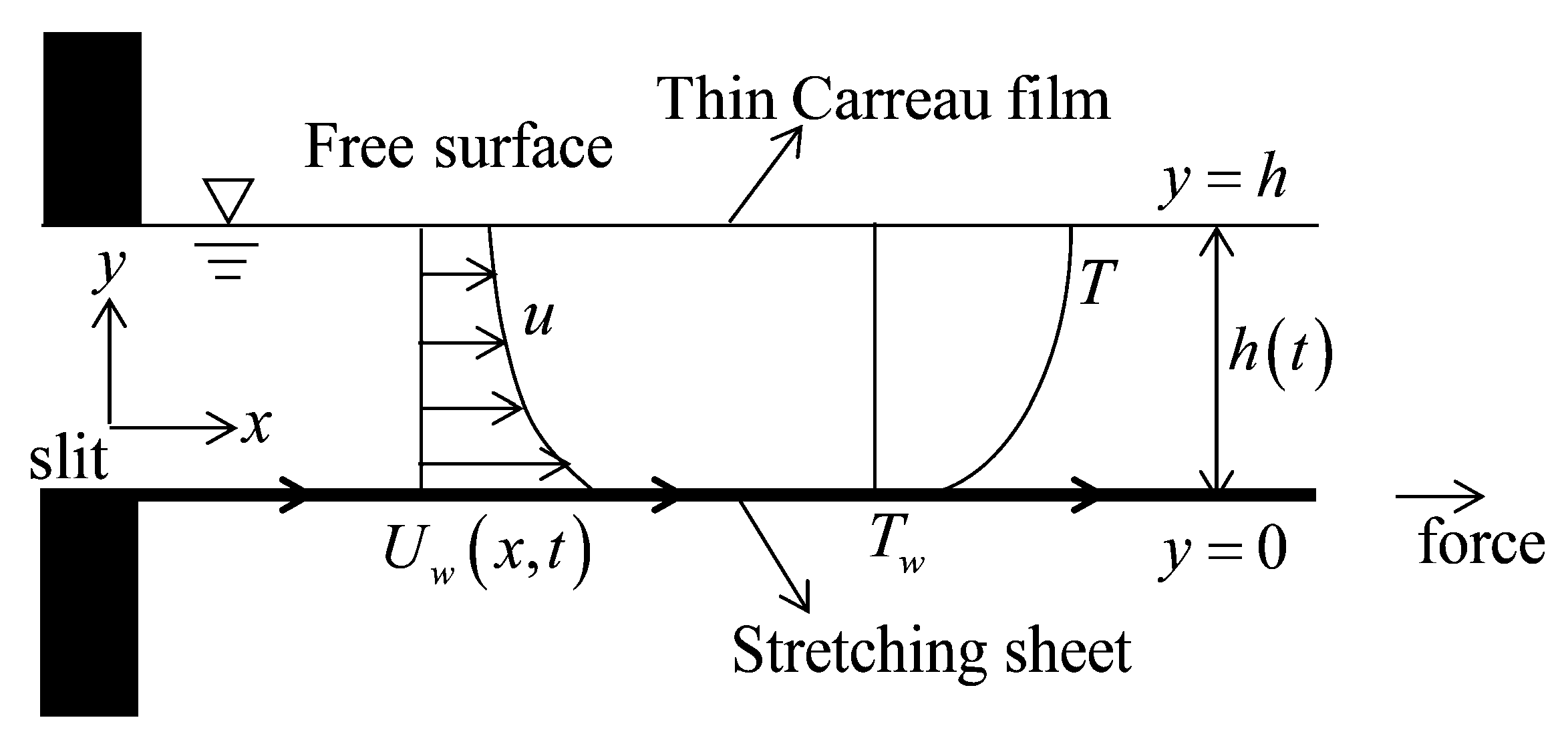
We are focused with an incompressible two–dimensional unsteady Carreau fluid flow confined by a thin liquid film of uniform thickness, $h\left(t\right)$ and a horizontal elastic sheet which is stretching from a narrow slit at the origin of the Cartesian coordinate system, as illustrated by Figure 1. The setup of the Cartesian coordinates is in a way where the $y-$ coordinate is normal to the $x-$ coordinate. The state of stretching sheet induce the Carreau fluid to flow within the thin film as the sheet stretched at $U_w\left(x,t\right)=\frac{bx}{\left(1-\alpha t\right)},$ where both $b$ and $\alpha$ are positive constants with dimension time^–1, $\alpha t\ne 1,$ and $b>0$ indicates the rate of stretching. The setup of $\alpha >0$ yields the constructive stretching rate, $b/\left(1-\alpha t\right)$ to upsurge with time. The surface of the sheet is permeable, and hence there is the mass velocity which is denoted by $V_w,$ wherein $V_w>0$ signifies suction while $V_w<0$ injection. The wall temperature is denoted by $T_w$ and $h\left(t\right)$ labels the film width. It is assumed that the end effects and gravity are negligible and the thickness of the film $h\left(t\right)$ is stable and uniform. It is worth mentioning that the boundary layer approximation is valid if, and only if, the thickness of the liquid film maintains its position without overlapping with the boundary layer thickness [40].

The Cauchy stress tensor for the Carreau fluid can be expressed as [45]

$$\tau =-p\mathbf{I}+\eta {\mathbf{A}}_1,$$

(1)

where

$$\eta ={\eta }_{\infty }+\left({\eta }_0-{\eta }_{\infty }\right){\left[1+{\left(\lambda \dot{\gamma }\right)}^2\right]}^{\frac{n-1}{2}},$$

(2)

wherein $\tau$ is the Cauchy stress tensor, $p$ is the pressure, $\mathbf{I}$ signifies the identity tensor, ${\eta }_0$ implies the zero-shear-rate viscosity, ${\eta }_{\infty }$ is the infinite-shear-rate viscosity, $\lambda$ denotes the material time constant, and $n$ represents the power–law index. The shear rate which is symbolized by $\dot{\gamma }$ can be conveyed as

$$\dot{\gamma }=\sqrt{\frac{1}{2}{\displaystyle \sum _j{\displaystyle \sum _j{\dot{\gamma }}_{ij}{\dot{\gamma }}_{ij}}}}=\sqrt{\frac{1}{2}\mathsf{\Pi }}=\sqrt{\frac{1}{2}\mathrm{tr}\left({\mathbf{A}}_1\right)}.$$

(3)

The second invariant strain rate tensor denoted by $\mathsf{\Pi }$ and ${\mathbf{A}}_1$ which implies the Rivlin–Ericksen tensor can be defined as

$${\mathbf{A}}_1=\left(\mathrm{grad}\mathbf{V}\right)+{\left(\mathrm{grad}\mathrm{V}\right)}^{\mathrm{T}}.$$

(4)

As been recommended by Boger [50], we consider the most practical cases where ${\eta }_0\gg {\eta }_{\infty }.$ Normally, the value of ${\eta }_{\infty }$ is determined by the extrapolation procedure or chosen to be zero (suggested theoretical value) [50]. We take the value of ${\eta }_{\infty }$ to be zero and thus Equation (1) simply becomes

$$\tau =-p\mathbf{I}+{\eta }_0{\left[1+{\left(\lambda \dot{\gamma }\right)}^2\right]}^{\frac{n-1}{2}}{\mathbf{A}}_1.$$

(5)

The Carreau model exhibits the shear thinning or pseudoplastic characteristics when the value of the power–law index lies within $0<n<1$. The Carreau model reveals the shear thickening or dilatant feature when $n>1$. Under these assumptions, the governing liquid film flow of the Carreau fluid can be written as

$$\frac{\partial u}{\partial x}+\frac{\partial v}{\partial y}=0,$$

(6)

$$\frac{\partial u}{\partial t}+u\frac{\partial u}{\partial x}+v\frac{\partial u}{\partial y}=\nu \frac{{\partial }^{2}u}{\partial y^2}{\left[1+{\lambda }^2{\left(\frac{\partial u}{\partial y}\right)}^2\right]}^{\frac{n-1}{2}}+\nu \left(n-1\right){\lambda }^2\frac{{\partial }^{2}u}{\partial y^2}{\left(\frac{\partial u}{\partial y}\right)}^2{\left[1+{\lambda }^2{\left(\frac{\partial u}{\partial y}\right)}^2\right]}^{\frac{n-3}{2}},$$

(7)

$$\frac{\partial T}{\partial t}+u\frac{\partial T}{\partial x}+v\frac{\partial T}{\partial y}=\kappa \frac{{\partial }^{2}T}{\partial y^2},$$

(8)

where $u$ and $v$ are the velocity components along the $x-$ and $y-$ directions, respectively, $\nu$ is the kinematic viscosity, $\lambda$ is a material time constant, $n$ signifies the power-law index, $T$ is the temperature, $\kappa =\frac{k}{\rho C_p},$ with $k$ is the thermal conductivity, $\rho$ is the density, and $C_p$ is the specific heat. The Equations (6)–(8) are accompanied by the boundary conditions as

$$\begin{array}{l}u=U_w\left(x,t\right), v=V_w, T=T_w \mathrm{at} y=0,\\ \mu \frac{\partial u}{\partial y}=\frac{\partial \chi }{\partial x}, \frac{\partial T}{\partial y}=0, v=\frac{dh}{dt} \mathrm{at} y=h,\end{array}$$

(9)

where $\chi$ is the surface tension which varies linearly with temperature [37] given as

$$\chi ={\chi }_0\left[1-\gamma \left(T-T_0\right)\right],$$

(10)

where ${\chi }_0$ is the surface tension at temperature $T_0$ and $\gamma$ is the positive fluid property. The wall temperature $\left(T_w\right)$ is defined as [37]

$$T_w=T_0-T_{ref}\left(\frac{b{x}^2}{2\nu }\right){\left(1-\alpha t\right)}^{-\frac{3}{2}},$$

(11)

where $T_0$ signifies the temperature at slit, and $T_{ref}$ embodies the reference temperature which can be taken as a constant reference temperature or as a constant temperature difference. The definition of $T_w$ imitates the circumstance where the sheet temperature decreases from $T_0$ at the slit in proportion to $x^2$ and the amount of temperature reduction along the sheet increases with time [37]. The expression for $U_w\left(x,t\right)$ and $T_w$ only valid for time $t<{\alpha }^{-1}$. The boundary condition when $y=h$ enforces a kinematic constraint of the fluid motion. Next, we introduce the similarity transformations as follows [26]:

$$\begin{array}{l}\psi =\sqrt{\frac{\nu b}{1-\alpha t}}\frac{x}{\beta }f\left(\zeta \right), u=\frac{\partial \psi }{\partial y}=\frac{bx}{1-\alpha t}{f}^{\prime }\left(\zeta \right), \\ v=-\frac{\partial \psi }{\partial x}=-\sqrt{\frac{\nu b}{1-\alpha t}}\beta f\left(\zeta \right), T=T_0-T_{ref}\left(\frac{b{x}^2}{2\nu }\right)\frac{1}{{\left(\sqrt{1-\alpha t}\right)}^3}\theta \left(\zeta \right),\end{array}$$

(12)

$$\zeta =\sqrt{\frac{b}{\nu }}\frac{y}{\beta \sqrt{1-\alpha t}},$$

(13)

where prime designates the derivative with respect to $\zeta ,$ $\psi \left(x,y,t\right)$ is the stream function, and $\beta ,$ the nonzero constant, is an unknown parameter representing the dimensionless film thickness. At the free surface, set $\zeta =1$ and (13) will take the form

$$\beta =\sqrt{\frac{b}{\nu \left(1-\alpha t\right)}}h\left(t\right),$$

(14)

which eventually gives

$$\frac{dh}{dt}=-\frac{\alpha \beta }{2}\sqrt{\frac{\nu }{b\left(1-\alpha t\right)}}.$$

(15)

Employing the similarity conversion as in (12) and (13) into the governing model (6)–(9) satisfies the continuity equation and the remaining equations are transformed as

$$\left[1+\frac{nW{e}^2{\left(f^{″}\right)}^2}{J}\right]{\left[1+\frac{W{e}^2{\left(f^{″}\right)}^2}{J}\right]}^{\frac{n-3}{2}}{f}^{‴}+J\left(f{f}^{″}-\frac{\sigma \zeta }{2}{f}^{″}-{f^{\prime }}^2-\sigma f^{\prime }\right)=0,$$

(16)

$${\theta }^{″}+\mathrm{Pr}J\left(f{\theta }^{\prime }-2f^{\prime }\theta -\frac{\sigma \zeta {\theta }^{\prime }}{2}-\frac{3\sigma \theta }{2}\right)=0,$$

(17)

along with the boundary conditions

$$\begin{array}{l}f\left(0\right)=S, f^{\prime }\left(0\right)=1, \theta \left(0\right)=1, \\ f\left(1\right)=\sigma /2, f^{″}\left(1\right)=M\theta \left(1\right), {\theta }^{\prime }\left(1\right)=0,\end{array}$$

(18)

while letting the constant mass transfer parameter, $S=-\frac{V_w}{\beta }\sqrt{\frac{1-\alpha t}{\nu b}},$ with the setting $S>0$ connotes suction and $S<0$ indicates the injection condition, $W{e}^2=\frac{{\lambda }^2{b}^3{x}^2}{\nu {\left(1-\alpha t\right)}^3},$ is the local Weissenberg number, $J={\beta }^2$ is an unknown constant to be calculated as a part of the problem, $M=\frac{\gamma {\chi }_0{T}_{ref}\beta }{\mu \sqrt{b\nu }}$ is the thermocapillarity number, $\mathrm{Pr}=\frac{\nu }{\kappa }$ is the Prandtl number, and $\sigma =\frac{\alpha }{b}$ is the dimensionless measure of unsteadiness to the stretching rate. It has to be noted that when $n=1$ and $We=0,$ the Carreau fluid model will reveal the Newtonian characteristics. Besides that, setting $S=M=We=0$ and $n=3$ in (16)–(18) reduces the present model to the thin film flow problem considered by Wang [26]. Also, by fixing $S=We=0$ and $n=3$ in (16)–(18), the thermocapillarity effect in a thin film flow problem solved by Noor and Hashim [39] is recoverable if the value of the Hartmann number in Equation (14) of [39] set to be zero. The physical quantities of interest in the present work are the local skin friction coefficient $\left(C_{fx}\right)$ and the local Nusselt number $\left(N{u}_x\right)$ which can be defined as

$$C_{fx}=\frac{{\tau }_w}{\rho {\left(U_w\right)}^2/2}, N{u}_x=\frac{q_{w}x}{k{T}_{ref}},$$

(19)

where the wall shear stress $\left({\tau }_w\right)$ and the heat flux from the surface of the sheet $\left(q_w\right)$ are given by [51]

$${\tau }_w={\left\{{\mu }_0\frac{\partial u}{\partial y}{\left[1+{\lambda }^2{\left(\frac{\partial u}{\partial y}\right)}^2\right]}^{\frac{n-1}{2}}\right\}}_{y=0}, q_w=-k{\left(\frac{\partial T}{\partial y}\right)}_{y=0},$$

(20)

By employing (12)–(13) and inducing (20) into (19) provides the following expression

$$C_{fx}{\mathrm{Re}}_x^{1/2}=2f^{″}\left(0\right){\left\{1+\frac{W{e}^2}{J}{\left[f^{″}\left(0\right)\right]}^2\right\}}^{\frac{n-1}{2}}, 2N{u}_x{\mathrm{Re}}_x^{-3/2}\beta {\left(1-\alpha t\right)}^{1/2}={\theta }^{\prime }\left(0\right).$$

(21)

The local Reynolds number defined as ${\mathrm{Re}}_x=\frac{x{U}_w\left(x,t\right)}{\nu }.$

3. Computational Scheme

The developed boundary value problem of (16)–(18) in the previous section was solved numerically via a built-in method in the MATLAB software, that is the bvp4c function. The MATLAB solver bvp4c solver, which was originated by Shampine et al. [52], incorporates the finite-difference program that prompts the three stages of Lobatto IIIa rule. The robust Lobatto IIIa rule belongs to the implicit Runge-Kutta methods and exercised the collocation method associated with the implicit trapezoidal method. Thus, the MATLAB solver bvp4c denotes the collocation method, which presents the C1-continuous solution with a fourth-order precision uniformly in the interval where the function is integrated. In the present work, the bvp4c routine can commence by defining the following new variables of

$$\begin{array}{l}y\left(1\right)=f, y\left(2\right)=f^{\prime }, y\left(3\right)=f^{″},\\ y\left(4\right)=\theta , \mathrm{and} y\left(5\right)={\theta }^{\prime }.\end{array}$$

(22)

By employing the variables in (22), the system of ordinary differential equations (16)–(18) can be written in the terms

$$\begin{array}{l}{f}^{\prime }=y\left(2\right),\\ f^{″}=y\left(3\right),\\ f^{‴}=\frac{J\cdot \sigma \cdot \zeta \cdot 0.5\cdot y\left(3\right)+J\cdot {\left(y\left(2\right)\right)}^2+J\cdot \sigma \cdot y\left(2\right)-J\cdot y\left(1\right)\cdot y\left(3\right)}{\left[1+\frac{n\cdot W{e}^2\cdot {\left(y\left(3\right)\right)}^2}{J}\right]{\left[1+\frac{W{e}^2\cdot {\left(y\left(3\right)\right)}^2}{J}\right]}^{\frac{n-3}{2}}},\\ {\theta }^{\prime }=y\left(5\right),\\ {\theta }^{″}=2\cdot \mathrm{Pr}\cdot J\cdot y\left(2\right)\cdot y\left(4\right)+0.5\cdot \mathrm{Pr}\cdot J\cdot \sigma \cdot \zeta \cdot y\left(5\right)+1.5\cdot \mathrm{Pr}\cdot J\cdot \sigma \cdot y\left(4\right)-\mathrm{Pr}\cdot J\cdot y\left(1\right)\cdot y\left(5\right),\end{array}$$

(23)

Accompanied with the boundary conditions (18) which is written as

$$\begin{array}{l}{y}_a\left(1\right)-S=0, y_a\left(2\right)-1=0, y_a\left(4\right)-1=0,\\ y_b\left(1\right)-\sigma /2=0, y_b\left(3\right)-M\cdot y_b\left(4\right)=0, y_b\left(5\right)=0.\end{array}$$

(24)

The subscripts ‘$a$’ and ‘$b$’ describe the position at the surface of the stretching sheet and the free surface, respectively. The relative tolerance has been fixed to $1\times {10}^{-10}$ throughout the computation process. The bvp4c function eases the computation process of the boundary value problems involving unknown parameters, and efficient in solving the boundary value problems even with the poor guesses [52]. However, a good initial guess is requisite to obtain multiple solutions. By using this clue, the present work has generated three different numerical solutions by using three sets of different initial guesses. The existence of the non-uniqueness solutions is common in a boundary value problem because the nonlinearity of the mathematical model in (16)–(18) and the variation of the respective governing parameters may lead to bifurcations in solutions which encourages the presences of the multiple solutions [53]. In this work, non-uniqueness solutions have been identified and are classified as the first, second, and third solutions. The first solution is a numerical solution which converged with a thin boundary layer whereas the second and third solutions converged with the thicker boundary layer. These solutions satisfy the boundary condition (18). Before the present numerical results discussed, it is important to validate the mathematical model as in (16)–(18) and measure the efficiency of the collocation method.

Table 1. Comparison values of $\beta$ and $f^{″}\left(0\right)$ when $\mathrm{Pr}=n=1$ and $We=S=M=0$.

$\mathit{S}$	$\mathit{\beta }$		${\mathit{f}}^{″}\left(0\right)$
	Wang [26]	Present Study	Wang [26]	Present Study
0.6	3.13125	3.131710	$-3.74233$	$-3.742786$
0.7	2.57701	2.576995	$-3.14965$	$-3.149614$
0.8	2.15199	2.151994	$-2.68094$	$-2.680966$
0.9	1.81599	1.815987	$-2.29683$	$-2.296825$
1.0	1.54362	1.543616	$-1.97238$	$-1.972385$

and

Table 2. Comparison values of $\beta ,f^{″}\left(0\right)$ and $-{\theta }^{\prime }\left(0\right)$ when $n=3,\mathrm{Pr}=1,We=S=0$ and $M=1$.

$\mathit{S}$	$\mathit{\beta }$		${\mathit{f}}^{″}\left(0\right)$		$-{\mathit{\theta }}^{\prime }\left(0\right)$
	Noor and Hashim [39]	Present Study	Noor and Hashim [39]	Present Study	Noor and Hashim [39]	Present Study
0.6	3.077525	3.180970	$-3.648093$	$-3.798725$	4.946056	5.077439
0.8	2.238349	2.230600	$-2.777115$	$-2.770430$	3.729232	3.733874
1.0	1.654829	1.653841	$-2.097875$	$-2.095761$	2.884973	2.886293
1.2	1.271942	1.271892	$-1.598689$	$-1.598526$	2.297023	2.297249
1.4	1.002731	1.002729	$-1.199091$	$-1.199085$	1.856868	1.856914
1.6	0.803335	0.803335	$-0.856981$	$-0.856982$	1.507663	1.507691

show the comparison of the numerical results with the previous analytic solutions, and there is a good agreement. This validates the present model and proves the accuracy of the collocation method in solving a boundary layer problem as the present results able to withstand the homotopy analysis method (HAM) which has been employed by Wang [26] and Noor and Hashim [39].

4. Results and Discussion

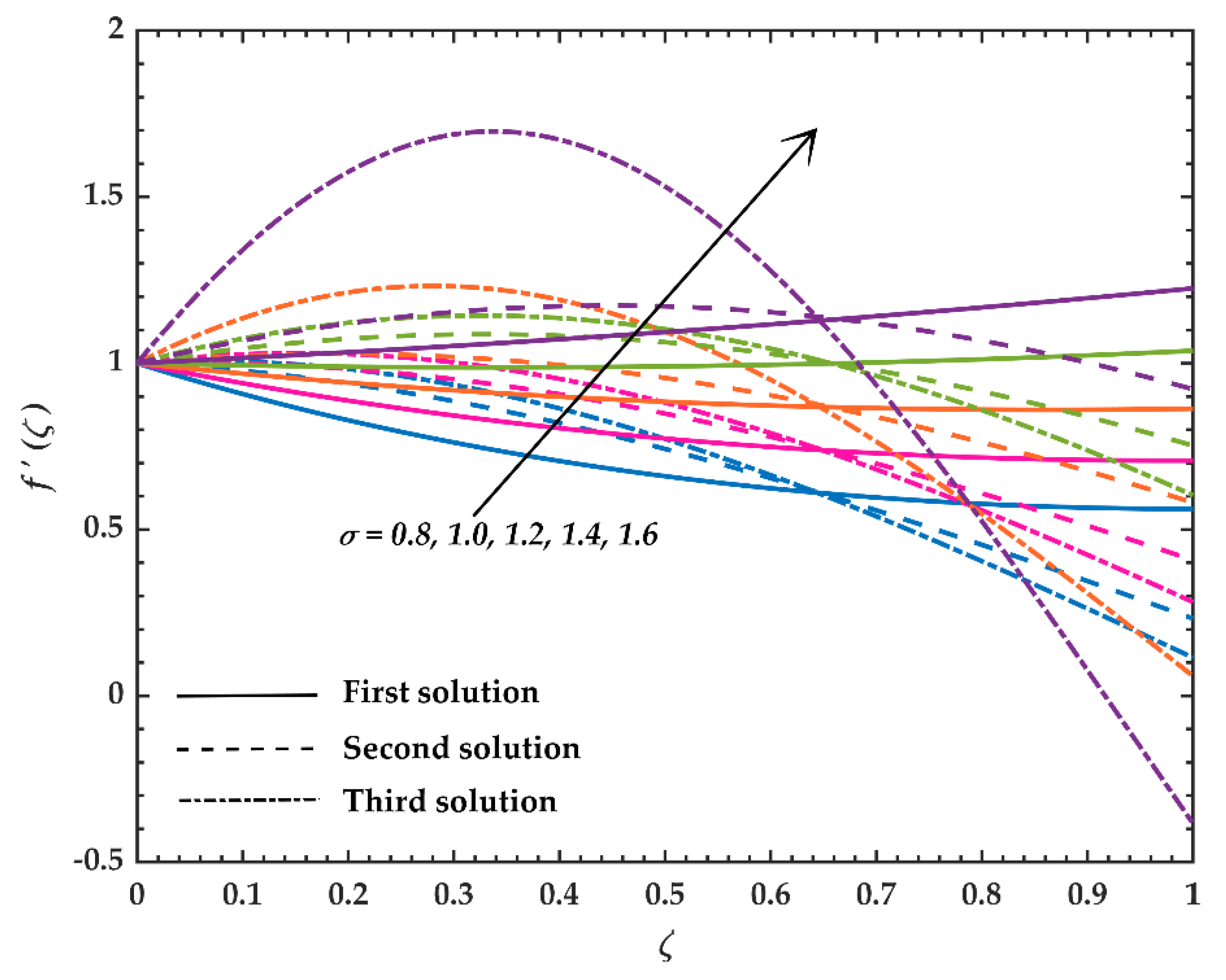
This section presents the numerical results in the form of the velocity and temperature profiles with a variation of the unsteadiness parameter $\left(\sigma \right)$, the thermocapillarity number $\left(M\right)$, and the constant mass transfer parameter $\left(S\right)$ within the range of $\left(0.8\le \sigma \le 1.6\right), \left(0.01\le M\le 2.0\right),$ and $\left(-0.3\le S\le -1.0\right),$ respectively. In the present study, the Prandtl number $\left(\mathrm{Pr}\right)$ has a fixed value of 30 as the interest is about the molten polymer. Meanwhile, the values of the local Weissenberg number $\left(We\right)$ and the power-law index $\left(n\right)$ are remained as 0.04 and 0.6, respectively. This section also organized in a way where the discussion of the first and second solutions is given initially, while the explanations of the third solution end up the section.

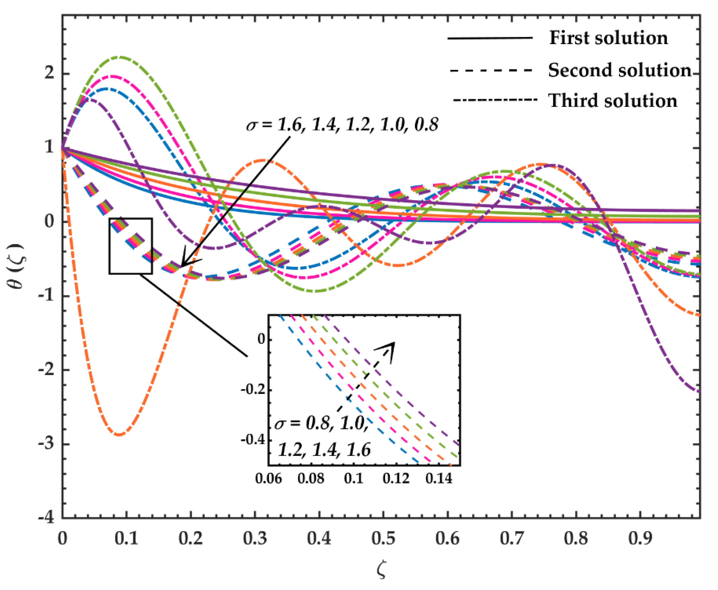
Figure 2 demonstrates the velocity profiles of the Carreau fluid when $\sigma$ varies past a stretching surface under the influence of injection at the rate of $-0.3$. The first and second solutions express an increment in the fluid velocity when the value of $\sigma$ increases from 0.8 to 1.6. Vajravelu et al. [54] have reported the unique solution with the similar result trend. Based on

Table 3. Value of $J$ as $\sigma$ varies at $\mathrm{Pr}=30,We=0.2,n=0.6,S=-0.3$ and $M=2$.

$\mathit{\sigma }$	$\mathit{J}$
	First Solution	Second Solution	Third Solution
0.8	1.0059106	$-0.9334169$	$-1.5042712$
1.0	0.4682307	$-0.7821466$	$-1.2449714$
1.2	0.2058215	$-0.6771271$	$-1.9809900$
1.4	0.0946128	$-0.5994718$	$-0.9362696$
1.6	0.0502582	$-0.5395827$	$-2.3099532$

, the increment in $\sigma$ gradually reduces the film thickness of the first solution. The decrement in the film thickness at the free surface increases the fluid velocity past the permeable stretching sheet, which then enhances the wall shear stress along with the stretching sheet. Consequently, the value of the reduced skin friction coefficient $\left(C_{fx}{\mathrm{Re}}_x^{1/2}\right)$ in

Table 4. Value of $C_{fx}{\mathrm{Re}}_x^{1/2}$ and ${\theta }^{\prime }\left(0\right)$ as $\sigma$ varies at $\mathrm{Pr}=30,We=0.2,n=0.6,S=-0.3$ and $M=2$.

$\mathit{\sigma }$	${\mathit{C}}_{\mathit{f}\mathit{x}}{\mathbf{Re}}_{\mathit{x}}^{1/2}$			${\mathit{\theta }}^{\prime }\left(0\right)$
	FS 1	SS 2	TS 3	FS 1	SS 2	TS 3
0.8	$-1.980577$	$-0.296318$	$0.369629$	$-6.407399$	$-15.643947$	$25.767820$
1.0	$-1.277002$	$0.141808$	$0.802004$	$-5.299440$	$-14.000526$	$27.249769$
1.2	$-0.665062$	$0.592954$	$3.288306$	$-4.064348$	$-12.656062$	$-101.360411$
1.4	$-0.149305$	$1.053797$	$1.746104$	$-3.054334$	$-11.503536$	$29.040625$
1.6	$0.304406$	$1.524980$	$8.210864$	$-2.385140$	$-10.487733$	$33.146586$

¹ FS = First solution. ² SS = Second solution. ³ TS = Third solution.

, increases and higher values of $C_{fx}{\mathrm{Re}}_x^{1/2}$ implies the growth in the frictional drag exerted on the stretching surface, which is not favorable in sustaining the laminar boundary layer flow. Intriguingly, the second solution in Table 3 which revealed the increment in the film thickness also records the increment in the values of $C_{fx}{\mathrm{Re}}_x^{1/2}$ like the first solution. Based on the values of $C_{fx}{\mathrm{Re}}_x^{1/2}$ for the first and second solutions in Table 4, a decrement in $\sigma$ elucidates that the stretching sheet found to exert the drag force on the Carreau fluid by expressing the negative values of $C_{fx}{\mathrm{Re}}_x^{1/2}.$ Next, Figure 3 displays the temperature profiles, and based on the first and second solutions, when the value of $\sigma$ increases, the fluid temperature increases and the heat flux from the surface of the sheet rises. Eventually, the thermal conductivity past the stretching sheet depreciates and increases the value of the local Nusselt number.

Table 5. Value of $J$ as M varies at $\mathrm{Pr}=30,We=0.2,n=0.6,S=-0.3$, and $\sigma =1.2$.

$\mathit{M}$	$\mathit{J}$
	First Solution	Second Solution	Third Solution
0.01	0.1654261	$-0.0237977$	$-0.1987100$
0.1	0.1681247	$-0.1855381$	$-1.1277911$
0.5	0.1785531	$-0.5951102$	$-3.2025872$
1.0	0.1891674	$-0.6234975$	$-1.1007880$
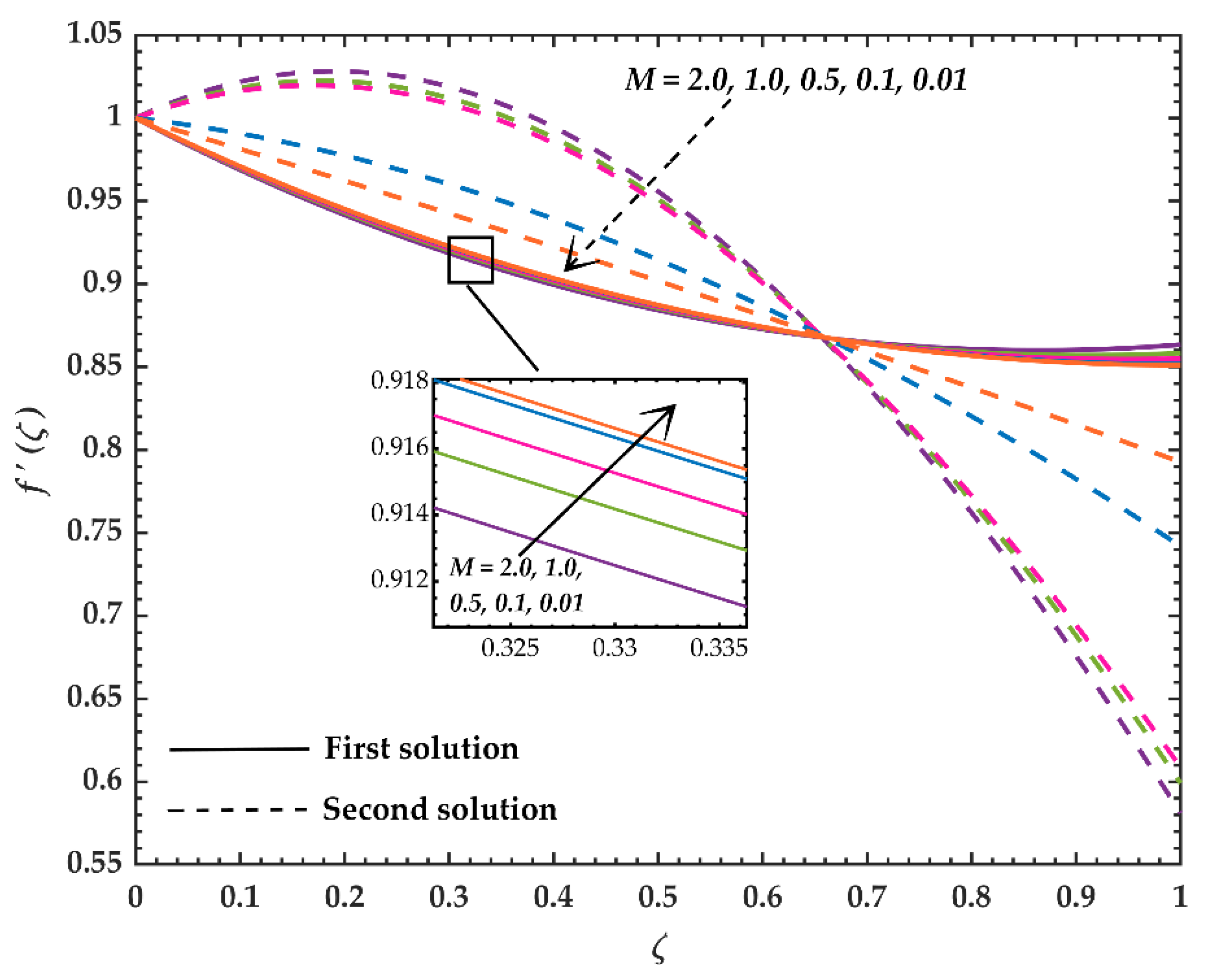
2.0	0.2058215	$-0.6771271$	$-1.0672621$

overviews the effect of the thermocapillarity number $\left(M\right)$ over $C_{fx}{\mathrm{Re}}_x^{1/2}$ and ${\theta }^{\prime }\left(0\right).$ The first solution in Table 5 exhibits the gradual increment in the film thickness $\left(J\right)$ when the values of M increases from 0.01 to 2.0. The increment in the film thickness then affects the fluid velocity to decrease, and this is depicted in Figure 4. The decreasing fluid velocity then reduces the wall shear stress past the stretching sheet and results in the decrement of $C_{fx}{\mathrm{Re}}_x^{1/2},$ as shown in

Table 6. Value of $C_{fx}{\mathrm{Re}}_x^{1/2}$ and ${\theta }^{\prime }\left(0\right)$ as $M$ varies at $\mathrm{Pr}=30,We=0.2,n=0.6,S=-0.3$ and $\sigma =1.2$.

$\mathit{M}$	${\mathit{C}}_{\mathit{f}\mathit{x}}{\mathbf{Re}}_{\mathit{x}}^{1/2}$			${\mathit{\theta }}^{\prime }\left(0\right)$
	FS 1	SS 2	TS 3	FS 1	SS 2	TS 3
0.01	$-0.613689$	$-0.372742$	$-0.127939$	$-3.714041$	$-39.195759$	$294.841558$
0.1	$-0.617140$	$-0.146453$	$1.377446$	$-3.739231$	$25.692494$	$782.037891$
0.5	$-0.630449$	$0.462043$	$8.923835$	$-3.833974$	$-40.763726$	$-40.729483$
1.0	$-0.643954$	$0.506981$	$1.326987$	$-3.926454$	$-22.672611$	$68.706145$
2.0	$-0.665062$	$0.592954$	$1.265005$	$-4.064348$	$-12.656062$	$28.245961$

¹ FS = First solution. ² SS = Second solution. ³ TS = Third solution.

. Noor and Hashim [39], and Rehman et al. [44] also have reported the decrement of the skin friction coefficient in their work. On the other hand, the second solution indicates the decrement in the value of $J$ past the unsteady stretching sheet. No one has reported such a trend before, and this suggests that an increment in the surface tension gradient have the potential to enhance the film thickness. The gradual increment in the film thickness triggers the speed of the fluid flow to increase, which then increases the wall shear stress and eventually, the value of $C_{fx}{\mathrm{Re}}_x^{1/2}$ increases. Besides that, the first solution in Figure 5 illustrates the decreasing trend of the fluid temperature when the thermocapillarity effect dominates near the free surface. When the fluid temperature decreases, the heat flow rate intensity from the surface of the stretching sheet declines. Thus, the thermal conductivity over the stretching surface increases and inducing the rate of heat transfer to decrease when M increases (see Table 6). These trends are in accordance with the findings given by [44]. The negative values of ${\theta }^{\prime }\left(0\right)$ elucidate that the heat energy is transferred from the fluid to the stretching sheet. Conversely, the second solution shows the decrement in $J,$ and the fluid temperature at the free surface found be increasing when $M$ increases after encountering some mild fluctuations across the boundary layer. As a result, the rate of convection heat transfer becomes inconsistent with the trend of increasing, decreasing, and increasing.

Table 7. Value of $J$ as $S$ varies at $\mathrm{Pr}=30,We=0.2,n=0.6,M=2$ and $\sigma =1.2$.

$\mathit{S}$	$\mathit{J}$
	First Solution	Second Solution	Third Solution
$-0.3$	$0.2058215$	$-0.6771271$	$-1.9809900$
$-0.5$	$0.0603109$	$-0.5696448$	$-1.1092403$
$-0.7$	$0.0246653$	$-0.5309704$	$-1.2876096$
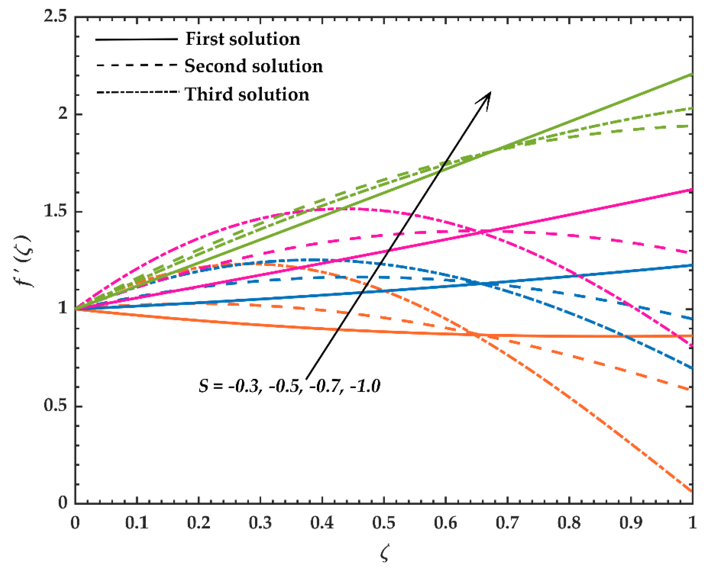
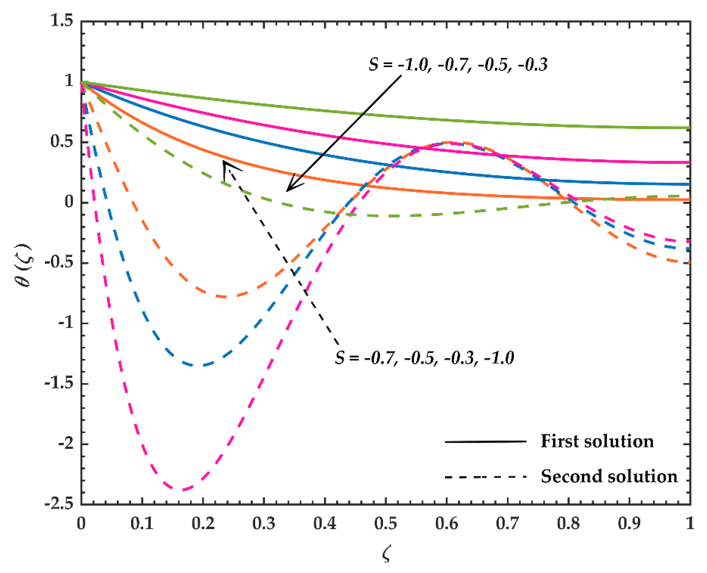
$-1.0$	$0.0072303$	$-0.2978425$	$-0.1952172$

displays the values of $J$ when the values $S$ decreases from $-0.3$ to $-1.0$. The decrement in $S$ explicates the increment in the injection intensity at the surface of the stretching sheet. The first solution shows that an increment in the injection strength reduces the film thickness at the free surface and affects the fluid velocity to increase steadily (see Figure 6). Rehman et al. [44] also has obtained the similar trend when $S$ decreases. The improvement in the fluid velocity, as shown in Figure 6, increases the skin friction at the surface of the stretching sheet, which then enhances the value of $C_{fx}{\mathrm{Re}}_x^{1/2}$ when $S$ decreases from $-0.3$ to $-1.0$ (see

Table 8. Value of $C_{fx}{\mathrm{Re}}_x^{1/2}$ and ${\theta }^{\prime }\left(0\right)$ as $S$ varies at $\mathrm{Pr}=30,We=0.2,n=0.6,M=2$ and $\sigma =1.2$.

$\mathit{S}$	${\mathit{C}}_{\mathit{f}\mathit{x}}{\mathbf{Re}}_{\mathit{x}}^{1/2}$			${\mathit{\theta }}^{\prime }\left(0\right)$
	FS 1	SS 2	TS 3	FS 1	SS 2	TS 3
$-0.3$	$-0.665062$	$0.592954$	$3.288306$	$-4.064348$	$-12.656062$	$-101.360411$
$-0.5$	$0.301583$	$1.430791$	$2.632399$	$-2.271308$	$-27.057939$	$287.943093$
$-0.7$	$1.052951$	2.453767	$4.824057$	$-1.471507$	$-50.930799$	$3901.196761$
$-1.0$	$1.535432$	$3.604139$	$3.337833$	$-0.733154$	$-4.841747$	$-8.748436$

¹ FS = First solution. ² SS = Second solution. ³ TS = Third solution.

). Interestingly, the second solution in Table 8 found to increase the film thickness at the free surface, and no one has reported this observation before. Even though the second solution displays the increment in $J,$ it does increases the value of $C_{fx}{\mathrm{Re}}_x^{1/2}$ when the impact of injection increases. From the aspect of the heat transfer, the first solution shows that the decrement in $S$ increases the fluid temperature and is disclosed in Figure 7. The effect of injection found to increases the amount of heat flux emitted from the stretching sheet, and this substantially augments the rate of convective heat transfer. Therefore, the values of ${\theta }^{\prime }\left(0\right)$ increase when the value of $S$ decreases. The second solution postulates the increment of the fluid temperature at the free surface after confronted the high oscillation across the boundary layer. Hence, the value of ${\theta }^{\prime }\left(0\right)$ decreases when $S$ varies from $-0.3$ to $-0.7,$ and then upsurges when $S$ varies from $-0.7$ to $-1.0$. Stronger injection effect at the surface of the stretching sheet increases the strength of the reverse or overshoot flow, which is shown in Figure 7 and Figure 8c [55]. The observed inflection points in Figure 7 and Figure 8c signify the flow instability, and this may yield the irregular rate of heat transfer past the stretching sheet.

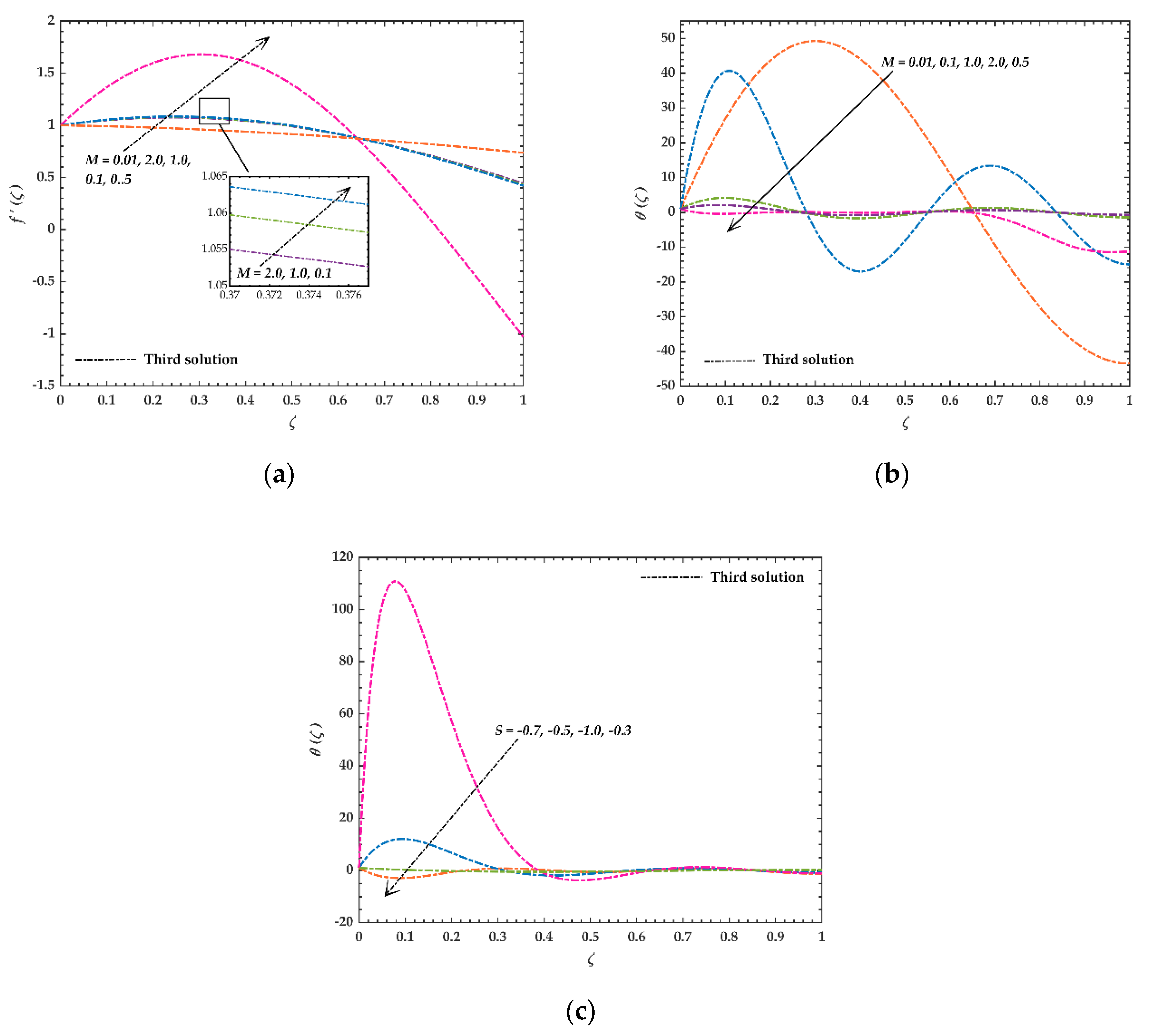
On the other hand, the remaining solution (third solution) yields the most negative values of $J$ when $\sigma ,M,$ and $S$ varies, and the most negative values can be set to zero [56]. When $J$ is set to zero, the momentum equation for the hydrodynamic boundary layer, as shown in Equation (16) is undefined and deleted from the problem matrix at this nodal point. Meanwhile, in the coating activities, the growth of the film is strictly dependent on the substrate flow over the stretching sheet (which is the Carreau fluid flow in the present work), and any changes occurring in the substrate vicinity will be reflected in the thin film thickness. Defects in the thin film flow such as a strong flow of divergence over the stretching sheet, or saddle points of attachment due to effect of surface tension, unsteadiness, or injection may yield the most negative film thickness. Therefore, when the most negative film thickness appeared, one can predict a rupture in the process and contact occurs between the film and stretching sheet surfaces [56]. Based on the results of the physical quantities and profiles (see Figure 2, Figure 3, Figure 6 and Figure 8) of the third solution in the present work, it is clear that there is an abrupt increase in the velocity profiles and irregular rising and falling in the fluid temperature which results in the uneven trend (increase, decrease and increase) of $C_{fx}{\mathrm{Re}}_x^{1/2}$ and ${\theta }^{\prime }\left(0\right),$ respectively. Even the reported values of $J$ for the third solution showed a changing trend; for instance, the thickness increase, decrease, increase. These essentially suggest the defects (as been explained above) within the boundary layer region, which have the potential to interrupt the film growing process.

5. Conclusions

The present investigation was conducted to observe the effects of thermocapillarity and injection in the Carreau thin film flow and heat transfer past an unsteady stretching sheet. The appropriate similarity variables transformed the governing boundary layer model which was in the form of the partial differential equations into a system of ordinary differential equations to ease the computational process. The reduced form of the mathematical model was solved numerically by a collocation method, namely bvp4c function in the MATLAB software. Interestingly, this study reported triple solutions in thin-film flow problems for the first-time. However, only one solution (first solution) can be physically reliable since the other two solutions (second and third solutions) are not reliable with negative film thickness. An increase in the unsteadiness parameter and higher intensity of injection reduces the film thickness, which then increases the value of the skin friction coefficient and improves the rate of convective heat transfer past a permeable stretching sheet. Besides that, an increase in the thermocapillarity number increases the film thickness, which then depreciates the value of the skin friction coefficient and deteriorates the rate of convective heat transfer past a permeable stretching sheet. This remarkable contribution could be useful in improving the manufacturing and materials processing.

References

- Prandtl, L. Über Flussigkeitsbewegungen bei sehr kleiner Reibung. Verhandlg. III Intern. Math. 1904, 484–491. Available online: https://ci.nii.ac.jp/naid/20000989592/ (accessed on 12 June 2020).
- Sakiadis, B.S. Boundary-layer behavior on continuous solid surfaces: I. Boundary-layer equations for two-dimensional and axisymmetric flow. AICH J. 1961, 7, 26–28. [Google Scholar] [CrossRef]
- Sakiadis, B.S. Boundary-layer behavior on continuous solid surfaces: II. The boundary layer on a continuous flat surface. AICH J. 1961, 7, 221–225. [Google Scholar] [CrossRef]
- Crane, L.J. Flow past a stretching plate. Z. Angew. Math. Phys. 1970, 21, 645–647. [Google Scholar] [CrossRef]
- Carragher, P.; Crane, L.J. Heat transfer on a continuous stretching sheet. Z. Angew. Math. Phys. 1982, 62, 564–565. [Google Scholar] [CrossRef]
- Krishna, M.V.; Chamkha, A.J. Hall and ion slip effects on MHD rotating boundary layer flow of nanofluid past an infinite vertical plate embedded in a porous medium. Results Phys. 2019, 15, 102652. [Google Scholar] [CrossRef]
- Basha, H.T.; Sivaraj, R.; Reddy, A.S.; Chamkha, A.J. SWCNH/diamond-ethylene glycol nanofluid flow over a wedge, plate and stagnation point with induced magnetic field and nonlinear radiation–solar energy application. Eur. Phys. J. Spec. Top. 2019, 228, 2531–2551. [Google Scholar] [CrossRef]
- Rasool, G.; Zhang, T.; Chamkha, A.J.; Shafiq, A.; Tlili, I.; Shahzadi, G. Entropy generation and consequences of binary chemical reaction on MHD Darcy–Forchheimer Williamson nanofluid flow over non-linearly stretching surface. Entropy 2020, 22, 18. [Google Scholar] [CrossRef] [Green Version]
- Gorla, R.S.R.; Chamkha, A. Natural convective boundary layer flow over a nonisothermal vertical plate embedded in a porous medium saturated with a nanofluid. Nanosc. Microsc. Therm. 2011, 15, 81–94. [Google Scholar] [CrossRef]
- Magyari, E.; Chamkha, A.J. Combined effect of heat generation or absorption and first-order chemical reaction on micropolar fluid flows over a uniformly stretched permeable surface: The full analytical solution. Int. J. Therm. Sci. 2010, 49, 1821–1828. [Google Scholar] [CrossRef]
- Chamkha, A.J. Solar radiation assisted natural convection in uniform porous medium supported by a vertical flat plate. J. Heat Transf. 1997, 119, 89–96. [Google Scholar] [CrossRef]
- Chamkha, A.J.; Al-Mudhaf, A. Unsteady heat and mass transfer from a rotating vertical cone with a magnetic field and heat generation or absorption effects. Int. J. Therm. Sci. 2005, 44, 267–276. [Google Scholar] [CrossRef]
- Takhar, H.S.; Chamkha, A.J.; Nath, G. Combined heat and mass transfer along a vertical moving cylinder with a free stream. Heat Mass Transf. 2000, 36, 237–246. [Google Scholar] [CrossRef]
- Chamkha, A.J.; Takhar, H.S.; Soundalgekar, V.M. Radiation effects on free convection flow past a semi-infinite vertical plate with mass transfer. Chem. Eng. J. 2001, 84, 335–342. [Google Scholar] [CrossRef]
- Takhar, H.S.; Chamkha, A.J.; Nath, G. Unsteady three-dimensional MHD-boundary-layer flow due to the impulsive motion of a stretching surface. Acta Mech. 2001, 146, 59–71. [Google Scholar] [CrossRef]
- Chamkha, A.J.; Al-Mudhaf, A.F.; Pop, I. Effect of heat generation or absorption on thermophoretic free convection boundary layer from a vertical flat plate embedded in a porous medium. Int. Commun. Heat Mass 2006, 33, 1096–1102. [Google Scholar] [CrossRef]
- Ghalambaz, M.; Behseresht, A.; Behseresht, J.; Chamkha, A. Effects of nanoparticles diameter and concentration on natural convection of the Al2O3-water nanofluids considering variable thermal conductivity around a vertical cone in porous media. Adv. Powder Technol. 2015, 26, 224–235. [Google Scholar] [CrossRef]
- Chamkha, A.J. Hydromagnetic natural convection from an isothermal inclined surface adjacent to a thermally stratified porous medium. Int. J. Eng. Sci. 1997, 35, 975–986. [Google Scholar] [CrossRef]
- Reddy, M.G.; Rani, M.S.; Kumar, K.G.; Prasannakumar, B.C.; Chamkha, A.J. Cattaneo-Christov heat flux model on Blasius-Rayleigh-Stokes flow through a transitive magnetic field and Joule heating. Phys. A 2020, 548, 123991. [Google Scholar] [CrossRef]
- Cotto, D.; Duffo, P.; Haudin, J.M. Cast film extrusion of polypropylene films. Int. Polym. Proc. 1989, 4, 103–113. [Google Scholar] [CrossRef]
- Wang, C.Y. Liquid film on an unsteady stretching surface. Q. Appl. Math. 1990, 48, 601–610. [Google Scholar] [CrossRef] [Green Version]
- Usha, R.; Sridharan, R. The axisymmetric motion of a liquid film on an unsteady stretching surface. J. Fluids Eng. 1995, 117, 81–85. [Google Scholar] [CrossRef]
- Andersson, H.I.; Aarseth, J.B.; Braud, N.; Dandapat, B.S. Flow of a power-law fluid film on an unsteady stretching surface. J. Non-Newton. Fluid Mech. 1996, 62, 1–8. [Google Scholar] [CrossRef]
- Andersson, H.I.; Aarseth, J.B.; Dandapat, B.S. Heat transfer in a liquid film on an unsteady stretching surface. Int. J. Heat Mass Transf. 2000, 43, 69–74. [Google Scholar] [CrossRef]
- Chen, C.H. Heat transfer in a power-law fluid film over a unsteady stretching sheet. Heat Mass Transf. 2003, 39, 791–796. [Google Scholar] [CrossRef]
- Wang, C. Analytic solutions for a liquid film on an unsteady stretching surface. Heat Mass Transf. 2006, 42, 759–766. [Google Scholar] [CrossRef]
- Noor, N.F.M.; Abdulaziz, O.; Hashim, I. MHD flow and heat transfer in a thin liquid film on an unsteady stretching sheet by the homotopy method. Int. J. Numer. Meth. Fluids 2010, 63, 357–373. [Google Scholar] [CrossRef]
- Aziz, R.C.; Hashim, I. Liquid film on unsteady stretching sheet with general surface temperature and viscous dissipation. Chin. Phys. Lett. 2010, 27, 110202. [Google Scholar] [CrossRef]
- Aziz, R.C.; Hashim, I.; Abbasbandy, S. Flow and heat transfer in a nanofluid thin film over an unsteady stretching sheet. Sains Malys. 2018, 47, 1599–1605. [Google Scholar] [CrossRef]
- Aziz, R.C.; Hashim, I.; Alomari, A.K. Thin film flow and heat transfer on an unsteady stretching sheet with internal heating. Meccanica 2011, 46, 349–357. [Google Scholar] [CrossRef]
- Kumar, K.A.; Sandeep, N.; Sugunamma, V.; Animasaun, I.L. Effect of irregular heat source/sink on the radiative thin film flow of MHD hybrid ferrofluid. J. Therm. Anal. Calorim. 2020, 139, 2145–2153. [Google Scholar] [CrossRef]
- Tassaddiq, A.; Amin, I.; Shutaywi, M.; Shah, Z.; Ali, F.; Islam, S.; Ullah, A. Thin film flow of couple stress magneto-hydrodynamics nanofluid with convective heat over an inclined exponentially rotating stretched surface. Coatings 2020, 10, 337. [Google Scholar] [CrossRef] [Green Version]
- Tan, M.J.; Bankoff, S.G.; Davis, S.H. Steady thermocapillary flows of thin liquid layers. I. Theory. Phys. Fluids A 1990, 2, 313–321. [Google Scholar] [CrossRef]
- Arafune, K.; Hirata, J. Thermal and solutal Marangoni convection in ln-Ga-Sb system. J. Crystal Growth 1999, 197, 811–817. [Google Scholar] [CrossRef]
- Christopher, D.M.; Wang, B.X. Similarity simulation for Marangoni convection around a vapor bubble during nucleation and growth. Int. J. Heat Mass Transf. 2001, 44, 799–810. [Google Scholar] [CrossRef]
- Dandapat, B.S.; Ray, P.C. The effect of thermocapillarity on the flow of thin liquid film on a rotating disc. J. Phys. D Appl. Phys. 1994, 27, 2041–2045. [Google Scholar] [CrossRef]
- Dandapat, B.S.; Santra, B.; Andersson, H.I. Thermocapillarity in a liquid film on an unsteady stretching surface. Int. J. Heat Mass Transf. 2003, 46, 3009–3015. [Google Scholar] [CrossRef]
- Chen, C.H. Marangoni effects on forced convection of power-law liquids in a thin film over a stretching surface. Phys. Lett. A 2007, 370, 51–57. [Google Scholar] [CrossRef]
- Noor, N.F.M.; Hashim, I. Thermocapillarity and magnetic field effects in a thin liquid film on an unsteady stretching surface. Int. J. Heat Mass Transf. 2010, 53, 2044–2051. [Google Scholar] [CrossRef]
- Maity, S.; Ghatani, Y.; Dandapat, B.S. Thermocapillary flow of a thin nanoliquid film over an unsteady stretching sheet. J. Heat Trans-T ASME 2016, 138, 042401. [Google Scholar] [CrossRef]
- Sarojamma, G.; Vajravelu, K.; Sreelakshmi, K. A study on entropy generation on thin film flow over an unsteady stretching sheet under the influence of magnetic field, thermocapillarity, thermal radiation and internal heat generation/absorption. Commun. Numer. Anal. 2017, 2, 141–156. [Google Scholar] [CrossRef] [Green Version]
- Maity, S. Thermocapillary flow of thin liquid film over a porous stretching sheet in presence of suction/injection. Int. J. Heat Mass Transf. 2014, 70, 819–826. [Google Scholar] [CrossRef]
- Rehman, S.; Rehman, S.U.; Khan, A.; Khan, Z. The effect of flow distribution on heat and mass transfer of MHD thin liquid film flow over an unsteady stretching sheet in the presence of variational physical properties with mixed convection. Phys. A 2020, 551, 124120. [Google Scholar] [CrossRef]
- Rehman, S.; Idrees, M.; Shah, R.A.; Khan, Z. Suction/injection effects on an unsteady MHD Casson thin film flow with slip and uniform thickness over a stretching sheet along variable flow properties. Bound. Value Probl. 2019, 1, 26. [Google Scholar] [CrossRef] [Green Version]
- Myers, T.G. Application of non-Newtonian models to thin film flow. Phys. Rev. E 2005, 72, 066302. [Google Scholar] [CrossRef]
- Tshehla, M.S. The flow of a Carreau fluid down an incline with a free surface. Int. J. Phys. Sci. 2011, 6, 3896–3910. [Google Scholar]
- Ashwinkumar, G.P.; Sulochana, C. Numerical simulation of heat transfer characteristics in thin film flow of MHD dissipative Carreau nanofluid past a stretching sheet with CoFe2O4 nanoparticles. Int. J. Res. Eng. Technol. 2016, 5, 18–25. [Google Scholar]
- Khan, N.S.; Gul, T.; Kumam, P.; Shah, Z.; Islam, S.; Khan, W.; Zuhra, S.; Sohail., A. Influence of inclined magnetic field on Carreau nanoliquid thin film flow and heat transfer with graphene nanoparticles. Energies 2019, 12, 1459. [Google Scholar] [CrossRef] [Green Version]
- Iqbal, K.; Ahmed, J.; Khan, M.; Ahmad, L.; Alghamdi, M. Magnetohydrodynamic thin film deposition of Carreau nanofluid over an unsteady stretching surface. Appl. Phys. A-Mater. 2020, 126, 105. [Google Scholar] [CrossRef]
- Boger, D.V. Demonstration of upper and lower Newtonian fluid behaviour in a pseudoplastic fluid. Nature 1977, 265, 126–128. [Google Scholar] [CrossRef]
- Khan, M.; Azam, M. Unsteady boundary layer flow of Carreau fluid over a permeable stretching surface. Results Phys. 2016, 6, 1168–1174. [Google Scholar] [CrossRef] [Green Version]
- Shampine, L.F.; Gladwell, I.; Thompson, S. Solving ODEs with MATLAB; Cambridge University Press: New York, NY, USA, 2003; p. 166. [Google Scholar]
- Schlicthing, H.; Gersten, K. Boundary-Layer Theory, 9th ed.; Springer Nature: Berlin, Germany, 2017; p. 99. [Google Scholar]
- Vajravelu, K.; Prasad, K.V.; Ng, C.O. Unsteady flow and heat transfer in a thin film of Ostwald-de Waele liquid over a stretching surface. Commun. Nonlinear Sci. Numer. Simulat. 2012, 17, 4163–4173. [Google Scholar] [CrossRef] [Green Version]
- Ali, M.E. The effect of suction or injection on the laminar boundary layer development over a stretched surface. J. King Saud Univ. 1996, 8, 43–58. [Google Scholar] [CrossRef]
- Dowson, D.; Priest, M.; Dalmaz, G.; Lubrecht, A.A. Tribological Research and Design for Engineering Systems; Elsevier: Amsterdam, The Netherlands, 2003; p. 581. [Google Scholar]
Figure 1.
Schematic diagram of the thin film flow along a stretching sheet.
Figure 2.
Velocity profiles, when , and as varies.
Figure 3.
Temperature profiles, when and as varies.
Figure 4.
Velocity profiles, when and as varies.
Figure 5.
Figure 6.
Figure 7.
Figure 8.
(a) Velocity profiles, of the third solution when and as varies; (b) Temperature profiles, of the third solution when and as varies; (c) Temperature profiles, of the third solution when and as varies.