Heating Performance Analysis for Short-Term Energy Monitoring and Prediction Using Multi-Family Residential Energy Consumption Data

Abstract

Many smart apartments and renovated residential buildings have installed Smart Meters (SMs), which collect interval data to accelerate more efficient energy management in multi-family residential buildings. SMs are widely used for electricity, but many utility companies have been working on systems for natural gas and water monitoring to be included in SMs. In this study, we analyze heating energy use data obtained from SMs for short-term monitoring and annual predictions using change-point models for the coefficient checking method. It was found that 9-month periods were required to search the best short-term heating energy monitoring periods when non-weather-related and weather-related heating loads and heating change-point temperatures are considered. In addition, the 9-month to 11-month periods were needed for the analysis to apply to other case study residences in the same high-rise apartment. For the accurate annual heating prediction, 11-month periods were necessary. Finally, the results from the heating performance analysis of this study were compared with the cooling performance analysis from a previous study. This study found that the coefficient checking method is a simple and easy-to-interpret approach to analyze interval heating energy use in multi-family residential buildings. It was also found that the period of short-term energy monitoring should be carefully selected to effectively collect targeted heating and cooling data for an energy audit or annual prediction.

1. Introduction

In a modern society, residential buildings are the primary source of national energy consumption, which use energy for occupants’ comfort and building system operations. Recently, the government of South Korea has developed an ambitious plan to improve building energy efficiency protocols. Thus, zero-energy buildings will be mandatory for all types of new constructions after 2030 [1]. In conformity with this, smart apartments and renovated residential buildings have installed Smart Meters (SMs), also called Advanced Metering Infrastructure (AMI), which collect interval energy use data to accelerate more efficient energy management in multi-family residential buildings.

AMI has great potential for energy use analysis applications by collecting and monitoring energy use data from buildings. The system combines software and hardware components, data management, and monitoring systems using a two-way real-time communication network [2,3]. The interval data from AMI or SMs can provide a high-resolution dataset of energy consumption, recording at regular intervals throughout a sub-hour, hour, or day, and is now available in many residential buildings based on real-time measurements.

Due to its detailed and disaggregated data information, interval energy use data from SMs offers a wide range of information about building operations and energy consumption for practitioners, providers, and customers. Previous studies have shown that fine-grained residential building consumption data can provide a better understanding of the lifestyle of occupants (e.g., electrical device usage patterns and occupant presence or absence) [4,5,6]. Furthermore, another study demonstrated that collecting data from buildings is useful to recognize electrical energy usage patterns, which allows energy suppliers and distribution system operators to understand electricity market signals and customer behavior [7]. Thus, interval energy use data can be imperative to identify occupants’ energy usage habits, to develop advanced energy performance prediction models, and to perform energy auditing for optimal energy management and operation in buildings.

Interval energy use data are normally used to develop different types of data-driven (or inverse) energy models (e.g., steady-state and dynamic models). According to the purpose of the analysis (e.g., prediction, auditing, and calibration), data-driven modeling methods and tools can be different. For example, steady-state prediction models (e.g., change-point linear regressions, multi-linear and combined regressions) can be used if time-lagged variables are not presented [8]. The Inverse Modeling Toolkit (IMT) (Version 1.0, ASHRAE, Atlanta, GA, USA) developed by The American Society of Heating, Refrigerating and Air-Conditioning Engineers (ASHRAE) is a useful tool for steady-state modeling development [9,10]. Dynamic models (e.g., machine learning) can be developed using detailed information from buildings systems, which require a more complicated and time-consuming process. Over recent years, many studies have conducted statistical analysis for machine learning techniques using interval data to identify energy usage patterns [11] and capture non-linear and complicated relationships [12].

In addition, the energy auditing field can make great use of interval energy use data. A home energy audit can depict a whole picture of home energy use to show how much energy was used, where energy was lost, and what should be fixed in homes to improve energy efficiency and the occupants’ comfort. This type of home energy audit is typically conducted before home retrofits [13]. Thus, for pre-retrofit homes, several studies have attempted to analyze residential energy consumption patterns using interval data.

In this study, we analyze interval heating energy use data for short-term monitoring and annual predictions using the change-point models. Natural gas (NG) monitoring has not yet been widely applied to SMs, so there were few studies on interval heating energy use data. In addition, few studies compared heating and cooling building energy performance using the interval data of heating and cooling energy consumption.

In the next section (i.e., Section 2), the previous studies are reviewed regarding analysis for interval energy use data using the change-point regression models and an energy audit for residential buildings. In Section 3, the overall approach of this study is described, including a description of the natural gas use data. The heating energy performance in multi-family residential buildings was analyzed using the coefficient checking method. The best interval data was used to search for the best monthly periods for short-term monitoring. Then, predicted annual heating energy use was compared with the measured one to verify the coefficient checking method. Next, a comparison between the heating and cooling energy use data was conducted to find the best periods for short-term monitoring. These results are presented in Section 4, and they are discussed in Section 5. The conclusion and contributions of this study are described in Section 6.

2. Literature Review

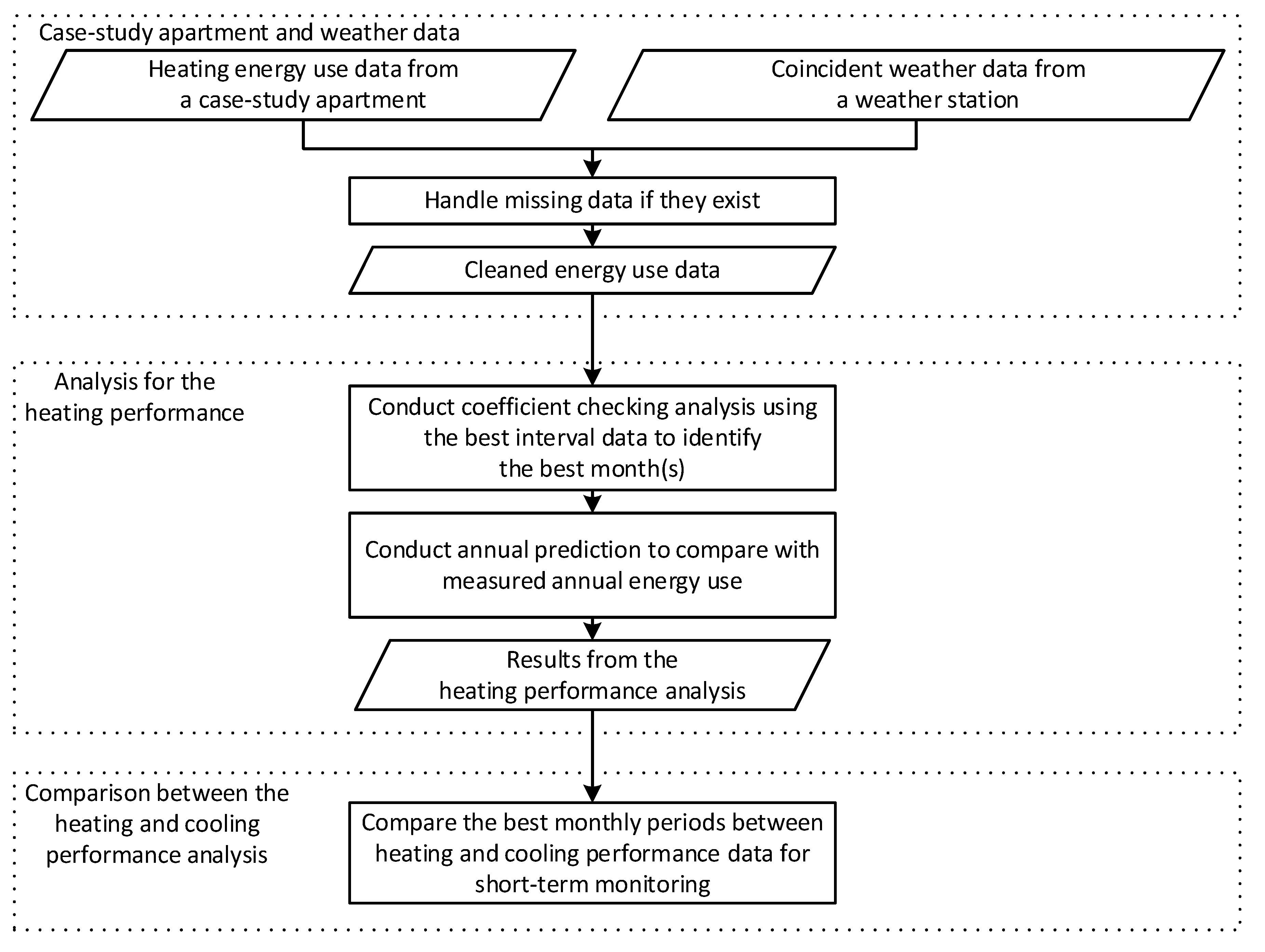
We found several studies conducted for the use of different energy data intervals to analyze building operations and energy consumption. The previous studies widely used the change-point linear regression models for their analyses.

One study [14] used hourly interval energy consumption data of 35 commercial buildings to identify anomalies in the energy use. A three parameter (3P) change-point model was used with two other models of neural networks and regression trees. The results from all three models showed good agreements. While one independent variable of outside air temperature data was used for the change-point model, four independent variables of binary work indicator, wind speed, solar radiation, and outside air temperature data were used for the other two models.

Another study developed change-point models using daily interval energy data of 45 air-conditioning systems located in the houses in Texas [15]. Their analysis found that the change-point model is a quick and simple approach for diagnosing problems and performing energy audits to analyze residential energy use. In addition, a calibrated simulation model was used to estimate the impact of energy saving measures. Other researchers also used calibrated simulations for single-family residential dwellings in a hot and humid climate using a 3P change-point model for monthly energy consumption data [16]. Their results showed that the strength of the 3P coefficients was that they characterize physical and operational characteristics of the building. Monthly energy use data was also used to develop the change-point models along with outlier detection methods on residential energy consumption prediction [17]. The results showed that the change-point models could outperform neural network models when monthly interval data was used.

In previous literature, while change-point models have been widely employed for building energy use analyses, other studies covered improved change-point models or other advanced methods. For example, one study developed an improved 3P cooling change-point model for daily aggregate cooling load from about 800,000 residential and commercial buildings in Abu Dhabi, United Arab Emirates [18]. They used additional humidity and solar irradiation terms for the model to predict cooling loads and the results were used as a predictive and planning tool.

Another study included neural network, Gaussian mixture regression, Gaussian process regression, and change-point regression approaches using daily and hourly energy consumption data from an office [19]. The study predicted the energy consumption based on statistical metrics. The results identified that the differences between the four inverse models were insignificant. In addition, the researchers developed a novel hybrid system for short-term load forecasting [20]. The hybrid system included a data pre-processing, multi-objective Salp Swarm, and interval prediction modules. The system was verified using half-hourly data. Another study suggested Lambda-based architecture to conduct two-level short-term load forecasting for hourly interval data [21]. The study found that the accuracy of the two-level forecasting approach was better than the one-level approach. Other researchers conducted big data analysis for 2.9 million heating plants from Lombardy, Italy [22]. Using the measured data, they analyzed the heating performance of the installed systems in the region, which could even help energy policy makers and planners. Even though many studies proposed advanced methods for building energy use analysis, when considering the simplicity of the inverse models, the change-point model provides the best balance between the accuracy and effort of the analysis.

The monitoring period of interval energy use data is also important because it affects the accuracy of the analysis results. However, long-term monitoring is costly and requires a lot of resources from the building operators and occupants. Thus, if short-term monitoring can meet the accuracy of annual energy performance verifications, it would save the year-long monitoring cost. Previous studies found that energy use data collected for less than a year was sufficient to determine a baseline model for analyzing annual energy use [23,24]. The researchers showed that two weeks of hourly interval data, along with long-term utility data, could accurately predict annual energy use for entire buildings [23]. Their analysis found that the monitoring period was important, and the swing seasons were the best periods to collect data. Another study proposed the dry-bulb temperature analysis (DBTA) ranking approach to identify the best monitoring period to achieve accurate inverse models for energy performance in buildings [24]. The results from the DBTA method provided a simple way of ranking different months of the year as starting points for monitoring according to the number of subsequent months required to collect enough data to develop accurate inverse models. The study found that short-term monitoring could generate predictive models for long-term building energy performance within acceptable accuracy levels.

Despite the success of the previous studies using interval energy consumption data, the analyses have not focused on effectively finding short-term monitoring periods regarding non-weather-related and weather-related energy use. In addition, they have not compared the results between heating and cooling energy use data. Therefore, in this paper, we used the coefficient checking method [25], which improved the DBTA method, with a heating change-point model for heating-related short-term monitoring for residences in an apartment. The change-point modeling approach was selected for this study because it is a simple, intuitive, and easy-to-interpret method for analyzing heating energy use performance, particularly for the heating energy usage in multi-family residential buildings. Short-term monitoring periods were carefully selected to effectively collect targeted data for an energy audit or an annual prediction, which is important for data-driven models. Furthermore, a comparison between the heating and cooling energy performance was also conducted for short-term monitoring periods.

3. Methods

Figure 1 shows the overall approach of this paper. First, heating energy use (i.e., natural gas use) data was obtained from a case study apartment, and the corresponding outside air temperature data was also used [26]. Second, we used the coefficient checking method [25] to identify the best monthly periods, with respect to the month of the year, for short-term monitoring of weather-related (i.e., weather-dependent) and non-weather-related (i.e., weather-independent) natural gas use. Annual predictions were also conducted for the analysis. Third, we compared the best monthly periods of short-term monitoring between the performance of heating and cooling energy use data.

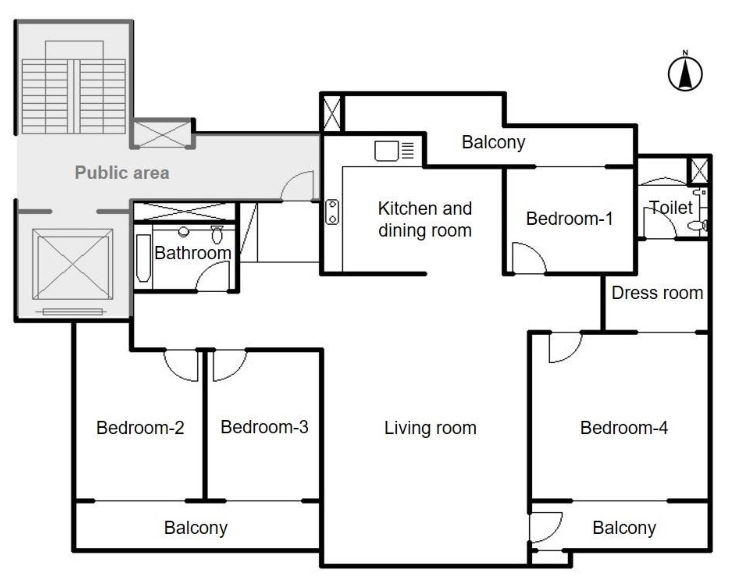
3.1. Case Study Apartment and Weather Data

A 14-story high-rise apartment building was selected for this study. Figure 2 shows a floor plan for one of the case study residences in the apartment building. Three bedrooms and one living room face the south, and one kitchen and dining room and one bedroom face the north. There are the balconies facing the north and south, respectively. 50 residences in the apartment have the same building configuration and building characteristics. However, half of the residences have the mirrored building configuration for the floor plan.

A summary of the case study information is shown in

Table 1. Characteristics of the 50 case study residences.

Construction Year	Insulation R-Value (m2-K/W)	Conditioned Floor Area (m2)/Unit	Occupancy/ Building System Type	# of Excluded Homes	Annual Average Natural Gas Use (kW h) of 49 Homes
2009	2.13 (Exterior wall) 0.33 (Exterior window) 2.86 (Interior wall) 1.23 (Interior floor)	142	Various	1	5070

. The high-rise apartment was built in 2009. The insulation R-values of exterior walls, exterior windows, interior walls, and interior floors were 2.13, 0.33, 2.86, and 1.23 m²-K/W, respectively. The total conditioned floor area of each residence was 142 m², and annual average natural gas use was 5070 kW h. Occupancy, building system, and/or appliance types and schedules were various even though the residences had the same building configuration, characteristics, and sizes. Thus, the different types were the major reasons for the maximum annual heating use of 13,979 kW h to the minimum of 491 kW h.

The daily natural gas use data from the apartment building in Seoul, South Korea, was obtained from 1 September 2009 to 31 August 2010. Natural gas was used for space heating only in the case study residences. The units of the natural gas use data were converted from Tonnage to kW h. The coincident outside air temperature (°C) was also collected during this period [26]. One residence of the apartment building was removed from the analysis because the residence did not use any natural gas. The analysis focuses on the interval natural gas use data from the remaining 49 residences. The number of Heating Degree Days (HDD) in South Korea was 2432 from the analysis results using data from 2001 to 2010 [27].

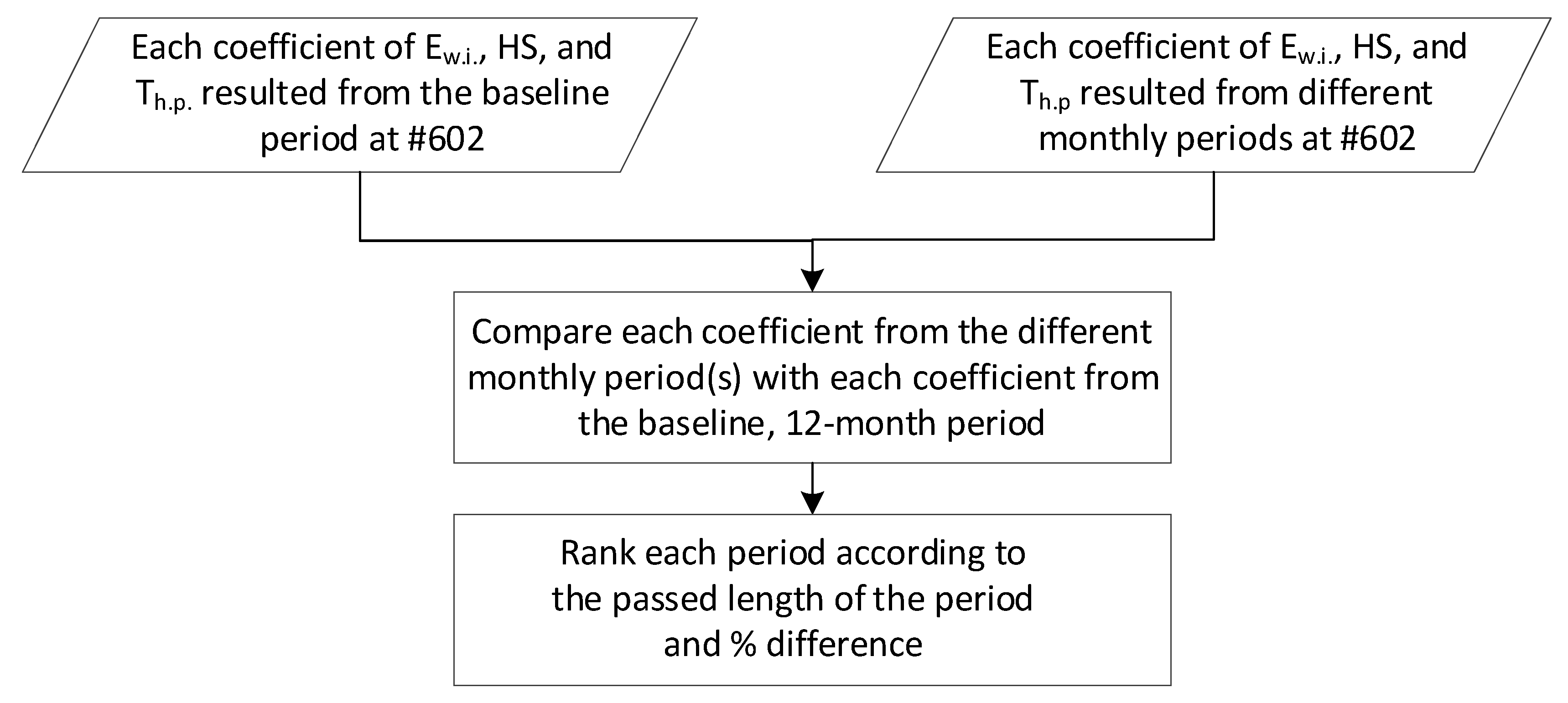
3.2. Analysis for the Heating Performance

For this paper, the Inverse Modeling Toolkit (IMT) [28] developed by ASHRAE was used. The three-parameter heating (3PH) change-point model is expressed in Equation (1).

$$E_{tot}=E_{w.i.}+HS{(T_{OA}-T_{h.p.})}^{-}$$

(1)

Here, E_tot is the total natural gas use, T_OA is the outdoor air temperature, E_w.i. is the non-weather-related natural gas use, HS is the heating slope, and T_h.p. is the heating change-point temperature. The notation $($ ${)}^{-}$ means that if T_OA is higher than T_h.p., then the value is changed to zero.

The coefficient of determination (R²) of Equation (1) and the Coefficient of Variation of the Root-Mean-Square Error (CV-RMSE) of Equation (2) were used to investigate the accuracy of the 3PH model.

$${\mathrm{R}}^2=\frac{{\sum }_i{(y_i-\overline{y})}^2-{\sum }_i{(y_i-{\widehat{y}}_i)}^2}{{\sum }_i{(y_i-\overline{y})}^2}$$

(2)

$$\mathrm{CV}-\mathrm{RMSE}=\frac{\sqrt{\frac{{\sum }_i{(y_i-\widehat{y_i})}^2}{\left(n-1\right)}}}{\overline{y}}\times 100(\%)$$

(3)

Here, $y_i$ is the measured heating (i.e., natural gas) use data, ${\widehat{y}}_i$ is heating use predicted by the 3P model, $\overline{y}$ is the average of the measured heating use data, and n is the number of heating use data.

A higher R² and lower CV-RMSE represent better accuracy of the 3PH model [8,29]. The statistical thresholds were chosen as shown in

Table 2. Thresholds for heating use data.

Interval Type	R2≥	CV-RMSE (%) ≤
Daily	0.25	50
Weekly	0.475	40
Monthly	0.70	30

, which are based on the thresholds defined in the previous study [29]. The calculated values of R² and CV-RMSE for the daily interval data were 0.25% and 40% respectively, and the values of R² and CV-RMSE for the monthly interval data were 0.70% and 20%, respectively. The report used these statistical limits for the case study of military residences. Since we assumed that natural gas use from normal residences could include more distributed heating energy use due to increased variations in occupant behaviors, we used a flexibility of +10% for the CV-RMSE thresholds of daily and monthly intervals. The values of R² and CV-RMSE for the weekly interval data were calculated using the daily and monthly thresholds through linear interpolation. After comparing the heating energy use of the 49 residences between the daily, weekly, and monthly average intervals, the best data was the weekly interval because of the 3PH models’ results—7, 19, and 18 residences passed the daily, weekly, and monthly thresholds (see Table 2). The previous study [25] also found that weekly interval data for cooling energy use was the best among the three intervals.

In addition, thresholds of ±100%, 2%, and 2% were used in the coefficient checking method for the weather-independent natural gas use ($E_{w.i.}$), the heating slope ($HS$), and the heating change-point temperature ($T_{h.p.}$) of the 3PH model, respectively. Using the weekly interval data from residence #602 of the case-study apartment building, the three thresholds of ±100%, ±2%, and ±2% were tested. The results showed that ±6.1% of the Normalized Mean Bias Error (NMBE) and ±0.9% of the CV-RMSE were observed according to the ±100%, ±2%, and ±2% changes of each coefficient from the 3PH model. The values of NMBE and CV-RMSE passed the limits from the ASHRAE Guideline 14 [30] (see

Table 3. Thresholds used for the annual heating prediction.

Interval Type	NMBE (%) ≤	CV-RMSE (%) ≤
Hourly	±10	Not Applicable (NA) for this paper
Daily	±8.33	50
Weekly	±6.67	40
Monthly	±5	30

). The best monthly periods were identified when the differences (%) of each coefficient were less than or equal to ±100%, 2%, and 2% compared to the corresponding 12-month coefficients. Based on the number of months and the differences in the coefficients (%), the best periods were ranked. The coefficient checking procedures for the heating energy use are summarized in Figure 3.

Finally, the predicted annual natural gas use was compared with the measured natural gas use. The best periods from the overall coefficient rank analysis were used for the comparison. The overall coefficient rank approach simultaneously used all the ±100%, 2%, and 2% thresholds for the three coefficients ($E_{w.i.}$, $HS$, and $T_{h.p.}$) to find the best overall short-term heating energy monitoring periods. In order to check the accuracy of the predicted annual natural gas use, the NMBE and CV-RMSE were used [30]. A lower NMBE indicates less error bias in the 3PH model. NMBE is defined according to the following equation:

$$\mathrm{NMBE}=\frac{\frac{{\sum }_i\left(y_i-\widehat{y_i}\right)}{\left(n-1\right)}}{\overline{y}}\times 100(\%)$$

(4)

Table 3 shows the statistical thresholds for the annual predictions. ASHRAE Guideline 14 suggests hourly and monthly limits using NMBE and CV-RMSE values [30]. The thresholds of NMBE for the daily and weekly interval data were calculated using linear interpolation from the hourly and monthly limits [19,30]. The values for the daily and weekly thresholds of CV-RMSE from Table 2 were used in this paper to include the flexibility of +10%.

3.3. Comparison between Short-Term Heating and Cooling Monitoring Performance

To further analyze the short-term monitoring periods, the results from this study were compared with the results from the previous paper [25]. The previous study published in this year developed the coefficient checking method using change-point models for interval cooling consumption data at the whole-building level. The same baseline period from 1 September 2009 to 31 August 2010 was used for the previous study. The previous study concluded that the coefficient checking method was useful to search the best periods for non-weather-related and weather-related short-term cooling energy monitoring. While the previous study used electricity use data, this study used natural gas use data for the coefficient checking method. Thus, in this study, the characteristics of heating consumption data were effectively compared with cooling data.

The best time periods for short-term monitoring of the heating energy use were compared with the best time periods for the cooling energy use. To effectively analyze the heating and cooling performance results, a graphical approach using bar graphs was developed, as shown in the figures of the Section 4.2. In order to compare the short-term heating and cooling monitoring performance among individual residences, several residences (units #301, #304, #503, #601, and #602) were selected. The residences were selected because they passed the thresholds of R² and CV-RMSE for both the weekly heating and cooling loads. Residence #602 was selected for the detailed coefficient checking analysis for both the heating and cooling energy use data.

4. Results

The main results from the coefficient checking method for heating energy use were the best short-term monitoring periods for non-weather-related and weather-related heating energy consumption. The shortened monitoring periods were useful to save time and costs to measure non-weather-related heating load (i.e., non-weather-related coefficient, representing the heating load affected by a range, oven, clothes dryer, etc.) and weather-related heating load (i.e., weather-related and change-point temperature coefficients, representing the heating load affected by a heating system, internal heat gain, heating setpoint, etc.). The predicted annual heating energy use from the change-point model was also compared to the measured annual usage to verify the accuracy of the coefficient checking method for residential heating loads. Then, we give a comparison between heating and cooling performance using the best short-term monitoring periods.

4.1. Short-Term Monitoring Analysis and Annual Prediction

4.1.1. Non-Weather-Related Heating Load

The best time periods were identified for the non-weather-related coefficient ($E_{w.i.}$) using the weekly interval data. The results of the $E_{w.i.}$ coefficient provides the best time period for data loggers to conduct non-weather-related heating load monitoring (kW h/day), such as range, oven, clothes dryer, etc. Compared to the non-weather-related cooling load from the previous study [25], the heating load was almost zero. In other words, practically, non-weather-related heating load did not occur during these monthly periods. This was because natural gas was used for space heating only (i.e., weather-related heating load) in the case study residences. However, if a residence has a natural gas-powered range, oven, clothes dryer, etc., non-weather-related heating load will be high.

The annual baseline period (i.e., from September to August) was rearranged into a consecutive 12-month period, from January to December. Then, using the ±100% threshold, the original coefficient of the non-weather-related heating load was checked by comparing it with each coefficient of the twelve 3PH models for consecutive monthly periods (e.g., January, January to February, January to March, etc.).

Table 4. Results from the ranking analysis for the non-weather-related coefficient ($E_{w.i.})$.

Starting Month	Ending Month	Period (Consecutive Months)	Average Difference (%)	Ranking
January	June, August, or November	6, 8, or 11 months	−17.6, −60.4, or 17.6	6
February	June, September, or December	5, 8, or 11 months	−23.6, −3.3, or 49.5	4
March	June or February	4 or 12 months	−45.1 or Not Applicable (NA)	10
April	August, November, or February	5, 8, or 11 months	−83.5, −51.6, or −16.5	5
May	September or February	5 or 10 months	−50.0 or −41.2	2
June	October or February	5 or 9 months	−70.9 or −35.2	1
July	October, April, or December	4, 10, or 12 months	−72.5, −63.7, or NA	9
August	October, April, or June	3, 9, or 11 months	−62.4, −40.7, or 20.9	3
September	October, June, or August	2, 10, or 12 months	−1.1, 18.7, or NA	8
October	September	12 months	NA	12
November	June or September	8 or 11 months	−36.3 or −3.3	7
December	July or December	8 or 12 months	−16.5 or NA	11

shows the results of this analysis according to the starting month, end month, monthly periods, average difference (%), and rank. Whenever the % difference was within the ±100% threshold, the month was noted in the end month and period columns. The longest periods were compared to assign relative ranks to consider reliable results. When the longest periods were the same between two or more different periods with the same starting month, the most recent period that passed the threshold was used in the comparison to assign a rank. If the former and the longest periods were the same, then the average % differences were compared. We calculated the average % difference with the % difference of each monthly period when the % difference stayed within the ±100% threshold.

Figure 4 visualizes the results from Table 4. The first rank (the starting month of June, indicated with the green cross mark) continued within the ±100% threshold (the maximum and minimum of the y-axis) since February (9 on the x-axis). The first rank also passed the threshold in October and November (i.e., 5 and 6 on the x-axis), but it did not pass the threshold in December and January (i.e., 7 and 8 on the x-axis). The second rank (the starting month of May, indicated with the black line-crossed mark) also stayed within the ±100% threshold since February (i.e., 10 on the x-axis). The second rank also passed the threshold in September, October, November, and December (i.e., 5–8 on the x-axis), but it did not pass the threshold in January (i.e., 9 on the x-axis). It is interesting to note that the best short-term monitoring periods (i.e., ranks #1, #2, and #3) for the weather-independent heating energy use included the summer months. In addition, the results show that the length of the periods was 9 months or longer, which was much longer than the periods observed for the non-weather-related cooling load (i.e., two or four months [25]), even though the weather-independent heating energy use was almost zero.

4.1.2. Heating Slope

The best time periods were identified for the coefficient of the weather-dependent natural gas use ($HS$) using the weekly interval data. The results of the heating slope provide the best monthly periods for data loggers to measure the weather-dependent heating system performance (kW h/day/°C). Lower heating slope values are obtained from more efficient heating systems, better duct and wall insulation, less duct leakage, and less envelope infiltration [31,32].

Table 5. Results from the ranking analysis for the heating slope coefficient ($HS$).

Starting Month	Ending Month	Period (Consecutive Months)	Average Difference (%)	Ranking
January	November	11 months	−1.17	8
February	January	12 months	Not Applicable (NA)	9
March	January	11 months	0.82	7
April	January	10 months	−0.41	3
May	January	9 months	0.82	1
June	May	12 months	NA	9
July	June	12 months	NA	9
August	June	11 months	−0.12	5
September	May	9 months	−1.02	2
October	September	12 months	NA	9
November	September	11 months	−0.23	6
December	September	10 months	−1.76	4

shows the ranking analysis results of the heating slope by starting month, ending month, the length of time periods, the average difference (%), and rank. Whenever the % difference remained within the ±2% threshold, the month was noted in the end month and period columns. When the ranking was the same between two or more cases, the average of the % differences for passed time periods was considered. In other words, we calculated the % average difference based on the % difference of each monthly period when the % difference stayed within the ±2% threshold. The 9-month period starting in May and ending in January obtained the highest rank, followed by the 9-month period starting in September and ending in May. Even though these two periods were both 9 months long, the period from May to January received the highest rank due to a lower % difference.

Figure 5 visualizes the results in Table 5. The figure indicates that the May mark for the first rank continued within the ±2% threshold from January (i.e., 9 on the x-axis), the September dot for the second rank continued within the ±2% thresholds from May (i.e., 9 on the x-axis), and the April mark for the third rank stayed within the ±2% thresholds from January (i.e., 10 on the x-axis). It should be noted that more than two marks did not occur close to the upper and lower thresholds before six consecutive months, which is similar to the trend observed with the marks of the weather-dependent cooling energy use [25]. Such a result occurs because finding the best short-term monitoring period in terms of weather-related heating load is difficult and requires the longest periods among the three coefficients. In addition, it should be interesting that the high ranking (i.e., #1–#3) short-term monitoring periods for weather-related heating load include even the summer months.

4.1.3. Heating Change-Point Temperature

We also found that the best monthly periods were found for the coefficient of the heating change-point temperature ($T_{h.p.}$) (i.e., the heating balance-point temperature) using the weekly interval data. The results of the change-point temperature coefficient can provide the best months for data loggers to measure the outside air temperature (°C) when the onset of heating-related energy use occurs. The internal heat gain, the heating load, and/or the heating setpoint may affect the heating balance-point temperature coefficient [31,32].

The results of the starting month, ending month, length of the time periods, average difference (%), and rank are shown in

Table 6. Results from the ranking analysis for the heating change-point coefficient ($T_{h.p.}$).

Starting Month	Ending Month	Period (Consecutive Months)	Average Difference (%)	Ranking
January	September	9 months	0.00	2
February	January	12 months	Not Applicable (NA)	8
March	January	11 months	0.00	5
April	January	10 months	0.00	4
May	April	12 months	NA	8
June	May	12 months	NA	8
July	June	12 months	NA	8
August	June	11 months	0.00	5
September	December or May	4 or 9 months	−1.55 or 1.07	1
October	September	12 months	NA	8
November	September	11 months	0.00	5
December	July or September	8 or 10 months	1.97 or 0.00	3

. Whenever the % difference remained within the ±2% threshold, the month was noted in the end month and the period columns. The longest periods were compared with each other to assign relative ranks to verify the accuracy and stability of the results. When two or more different cases have the same length of the time periods, the average % difference was applied. We obtained the average % difference based on the % differences from each monthly period when the % difference stayed within the ±2% threshold. The 9-month period starting in September and ending in May had the highest rank, followed by the 9-month period starting in January and ending in September. Even though they both have the same 9-month period, the period that started in September has a higher rank because it has one more month that passed the threshold.

Figure 6 gives a visual representation of the results from Table 6. The September mark for the first rank stayed within the ±2% threshold from January (i.e., 9 on the x-axis). This also passed the threshold on May (i.e., 4 on the x-axis), but it was not within the threshold between January and April (i.e., 1–3 on the x-axis). The January mark for the second rank stayed within the ±2% threshold from September (i.e., 9 on the x-axis). As previously mentioned, the period that was ranked #1 overcame period #2 since it contained one more month that passed the threshold. It is noteworthy that the length of the periods was longer or equal to 9 months from ranking #1 and ranking #2, which were much longer than the periods observed for the cooling energy use analysis (i.e., two and three months [25]). Therefore, this result shows that the coefficient checking method found less monitoring periods in terms of the cooling load. This was because the CV-RMSE for the 3P cooling models were much lower than the CV-RMSE for the 3P heating models.

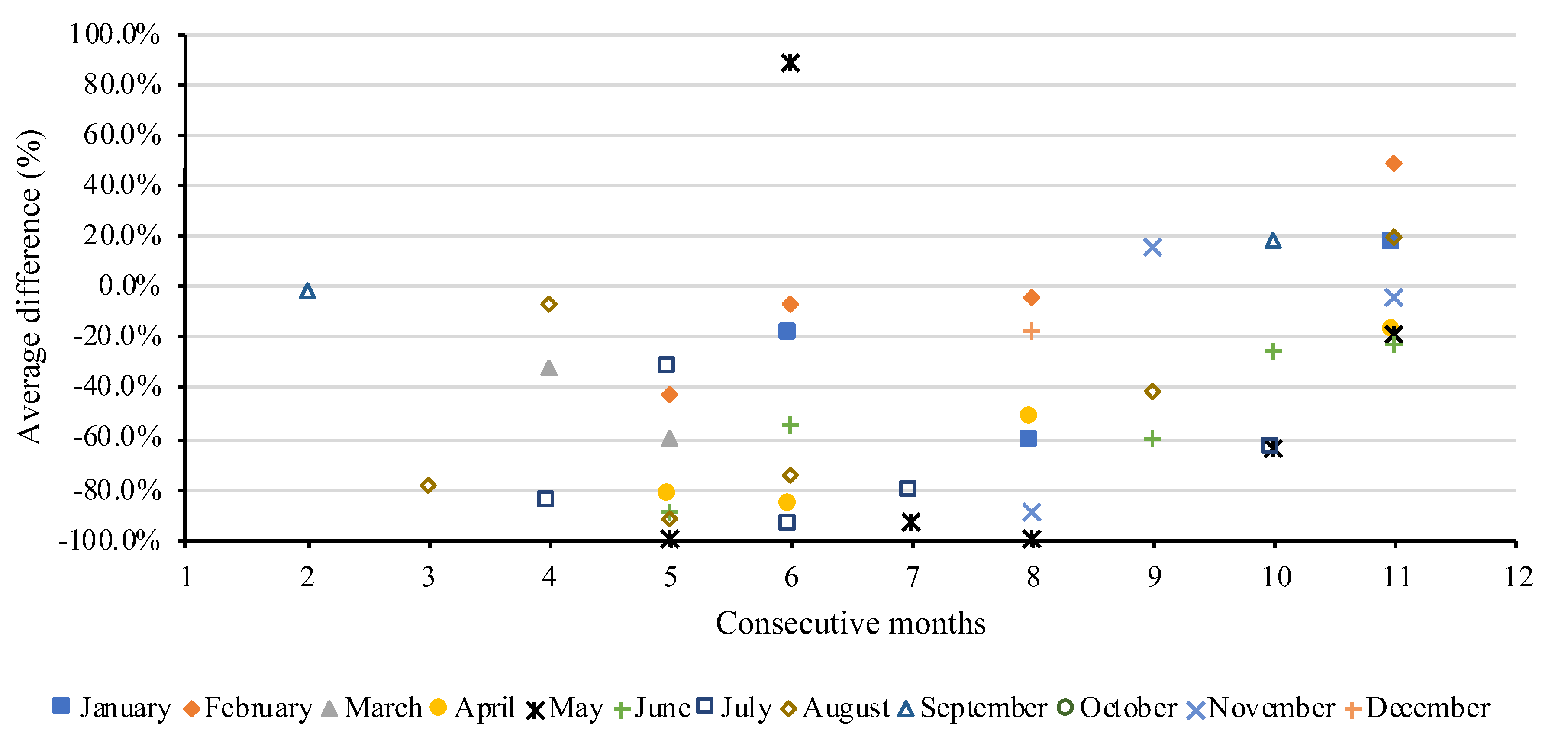
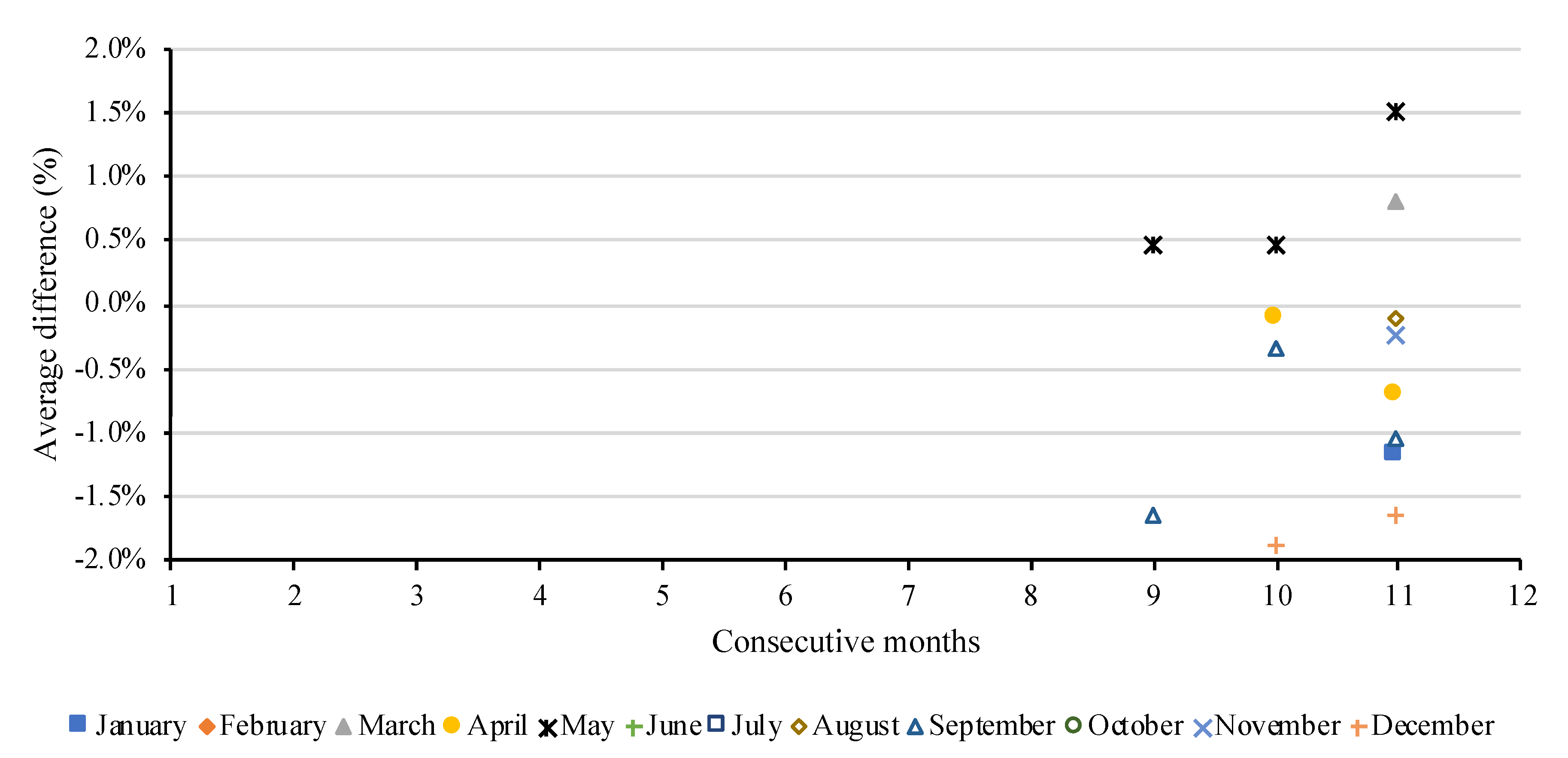
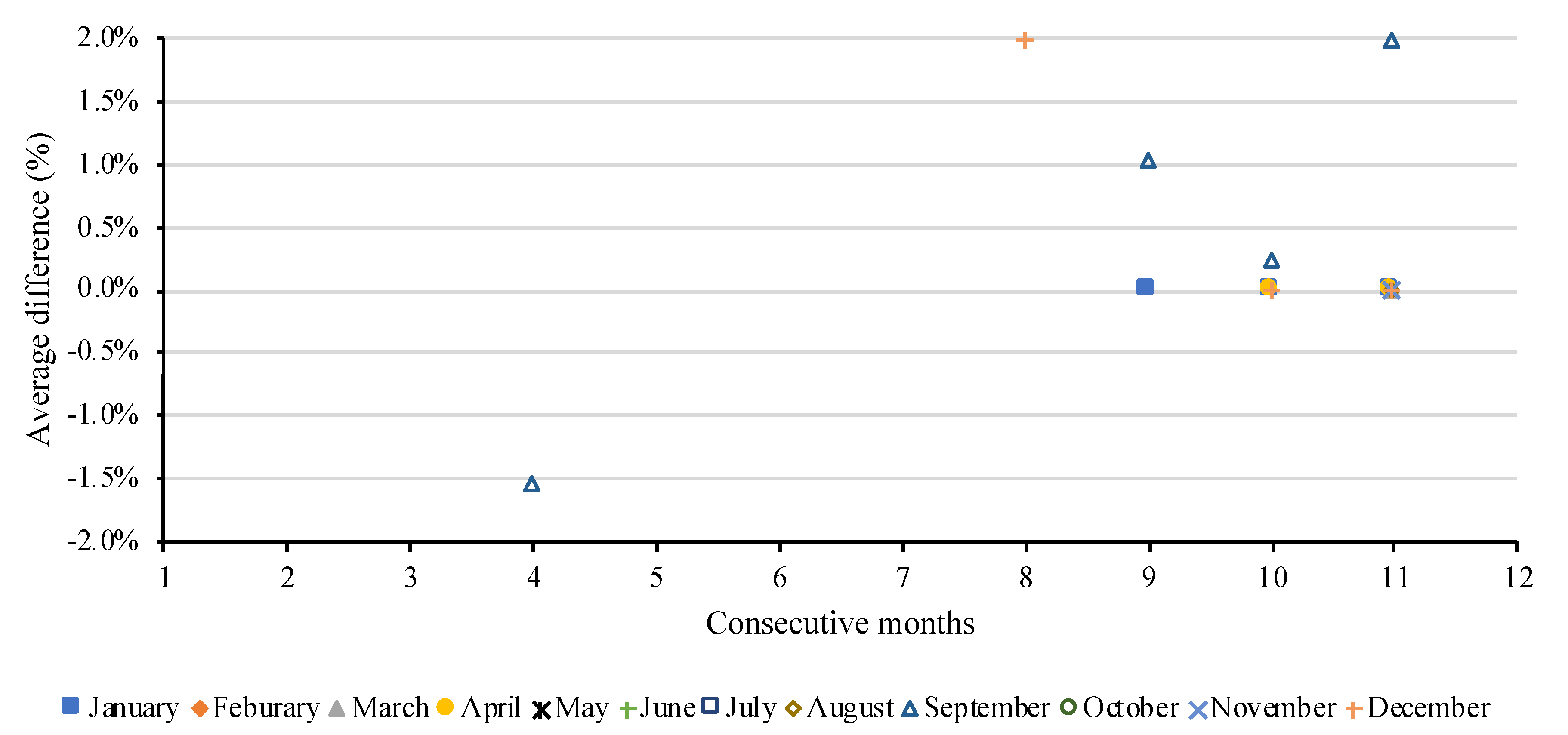
4.1.4. Overall Coefficient Rank Analysis and Annual Prediction

Overall coefficient ranks using all the ±100%, 2%, and 2% thresholds for the three coefficients ($E_{w.i.}$, $HS$, and $T_{h.p.}$) were applied to find the best short-term heating energy use monitoring period. This information can be used to identify the best period to install data loggers for measuring the overall residential heating performance. The same ranking approach from the previous subsections (i.e., Section 4.1.1, Section 4.1.2 and Section 4.1.3) was applied, except that an overall average difference (%) was used by calculating the overall average of the % differences from each coefficient.

Table 7. Results from the ranking analysis for all the three coefficients.

Start Month	End Month	Period	Overall Average Difference (%)	Ranking
January	November	11 months	5.47	2
February	January	12 months	Not Applicable (NA)	5
March	February	12 months	NA	5
April	February	12 months	NA	5
May	April	12 months	NA	5
June	May	12 months	NA	5
July	June	12 months	NA	5
August	June	11 months	6.92	3
September	June or August (except July)	10 or 12 months	6.19 or NA	4
October	September	12 months	NA	5
November	September	11 months	−1.18	1
December	November	12 months	NA	5

summarizes the results of the overall coefficient ranks. The best period was the 11-month period starting in November and ending in September. The second and third rankings were also 11-month periods, however, other months did not pass all the ±100%, 2%, and 2% thresholds. These results show that only one month can be skipped to measure the overall residential heating performance of an apartment building. On the other hand, the results from the previous study showed that four months can be skipped when monitoring the overall cooling performance [25].

In addition, the rankings #1–3 were applied to other residences in the case study apartment to predict annual heating energy use (see Section 4.1.5). The results from the overall coefficient rank analysis were very useful to analyze overall residential energy performance with reduced amounts of data, such as 11 months rather than 12 months.

4.1.5. Verification and Annual Prediction

In this section, we present the results from a verification process of the coefficient checking method and an annual prediction using the weekly natural gas use data. Residences #301, #304, #503, and #601 from the apartment building were selected for the verification process and to make the annual prediction because these units passed both the statistical indices of the goodness-of-fit thresholds. The verification process was conducted to check if the best heating periods, found in unit #602 with the coefficient checking method, can be applied to the other case study residences. If the best periods can be utilized for several residences for short-term monitoring, the time and money required to install the data loggers can be significantly reduced. As such, this test is important. The process assumes that the residences have similar characteristics, such as residences located in a high-rise building, and change-point models have the goodness-of-fit index for the residential interval data, such as the weekly heating energy use data.

The verification process results are shown in

Table 8. Results from the verification process.

Category	Coefficient	Ranking from #602	Applied Starting Month	Applied Ending Month	Applied Period	#301 Difference (%)	#304 Difference (%)	#503 Difference (%)	#601 Difference (%)
Individual	$E_{w.i.}$	1	June	February	9 months	−16.4	−67.3	−111.5	−26.7
		2	May	February	10 months			−149.2
		3	August	June	11 months			16.4
	$HS$	1	May	January	9 months	1.6	3.5	5.8	1.7
		2	September	May	9 months		−1.2	−0.8
	$T_{h.p.}$	1	September	May	9 months	0.4	−0.4	0.4	1.7
Overall	$E_{w.i.}$	1	November	September	11 months	46.2	−6.7	−80.5	−5.8
	$HS$					13.3	0.1	4.6	−3.1
	$T_{h.p.}$					−12.2	0.0	−4.1	3.4
	$E_{w.i.}$	2	January	November	11 months	3.5		−107.1	−40.0
	$HS$					−1.5		−8.7	1.2
	$T_{h.p.}$					0.0		4.1	0.0
	$E_{w.i.}$	3	August	June	11 months			16.4
	$HS$							−0.1
	$T_{h.p.}$							0.0

. The first column shows the category for individual coefficients when they passed each threshold, or overall coefficient when they passed all three thresholds. The highest rank to the lowest rank resulting from #602 were applied to the four residences in turn. When the rank passed the threshold, the % differences compared to the 12-month original coefficients were not calculated anymore, as shown in the last four columns of the table. It was found that all the residences (#301, #304, #503, and #601) passed the ±100%, 2%, and 2% thresholds within ranking #3 from the best periods at #602. For the heating weather-independent coefficient ($E_{w.i.}$), the 9-month period starting in June and ending in February (i.e., ranking #1) was acceptable for #301, #304, and #601. The 11-month period starting in August and ending in June (i.e., ranking #3) was acceptable for #503. For the heating slope coefficient ($HS$), the 9-month period starting in May and ending in January (i.e., ranking #1) was acceptable for #301 and #601. The 11-month period between August and the end of June (i.e., ranking #2) was acceptable for #503. For the heating change-point temperature coefficient ($T_{h.p.})$, the 9-month period starting in September and ending in May (i.e., ranking #1) was acceptable for all of the case study units. Thus, the 9-month period between September and the end of May could be an important period for the heating balance-point temperature heating slope coefficients.

Finally, for the overall coefficient approach, the 11-month period starting in November and ending in September (i.e., ranking #1) was acceptable for unit #304. The 11-month period between January and the end of November (i.e., ranking #2) was acceptable for residences #301 and #601. The 11-month period starting in August and ending in June (i.e., ranking #3) was acceptable for #503.

Then, using the best heating periods obtained from the overall coefficient rank analysis, annual predictions were calculated (see

Table 9. Results from the annual prediction analysis.

Residence	Category	Applied Starting Month	Applied Ending Month	Difference (%)			R2	CV-RMSE (%)	NMBE (%)	Monitored Annual Natural Gas (NG) Use (kW h)	Predicted Annual NG Use (kW h)	Annual Difference (%)
				${\mathit{E}}_{\mathit{w}.\mathit{i}.}$	$\mathit{H}\mathit{S}$	${\mathit{T}}_{\mathit{h}.\mathit{p}.}$
#602	Baseline	January	December	Not Appli-cable (NA)	NA	NA	0.89	31.7	0.6	3541.5	3468.2	−2.1
	Best period (Ranking #1)	November	September	−3.3	−0.2	0.0	0.89	31.8	0.9	3541.5	3458.6	−2.3
#301	Baseline	January	December	NA	NA	NA	0.92	32.6	0.2	6833.9	6873.5	0.6
	Best period (Ranking #2)	January	November	3.5	−1.5	0	0.92	32.7	1.7	6833.9	6775.3	−0.9
#304	Baseline	January	December	NA	NA	NA	0.95	22.7	−0.2	6006.7	5988.7	−0.3
	Best period (Ranking #1)	November	September	−6.7	0.1	0	0.95	22.8	−0.1	6006.7	5982.6	−0.4
#503	Baseline	January	December	NA	NA	NA	0.92	32.9	−0.1	6859.5	6914.9	0.8
	Best period (Ranking #3)	August	June	16.4	−0.1	0	0.92	32.8	−0.3	6859.5	6925.8	1.0
#601	Baseline	January	December	NA	NA	NA	0.93	26.1	−0.2	4496.3	4553.5	1.3
	Best period (Ranking #2)	January	November	−40	1.2	0	0.93	26.4	−1.1	4496.3	4590.8	2.1

). In other words, the best periods that resulted from the overall coefficient ranks in Table 8 were applied to the four residences. The category column shows the applied periods from the passed ranks. The 12-month baseline period was also applied to compare with the results from the best periods. Every case study unit passed the statistical indices for NMBE (±6.67%) and CV-RMSE (40%), as shown in Table 3.

In summary, the results showed that the coefficient checking method was effective for residences in the multi-family residential building type to identify the best monthly periods for non-weather-related and weather-related heating load, as well as heating change-point temperatures. This was very meaningful to show how the short-term energy monitoring period ranking results from one residence can be applied to other residences in the same apartment for non-weather-related, weather-related, and overall residential heating energy performance. It is worth noting that the previous study [25] found that residences should have similar change-point temperatures in order to obtain better results when the cooling coefficient checking method was used. For this study, residences #301, #304, #503, #601, and #602 had heating change-point temperatures of 17.6, 19.1, 17.6, 21.2, and 22.7 °C, respectively. Thus, the best monthly periods from the heating coefficient checking method were properly applied to each selected residence in the case study apartment due to the similar heating change-point temperatures.

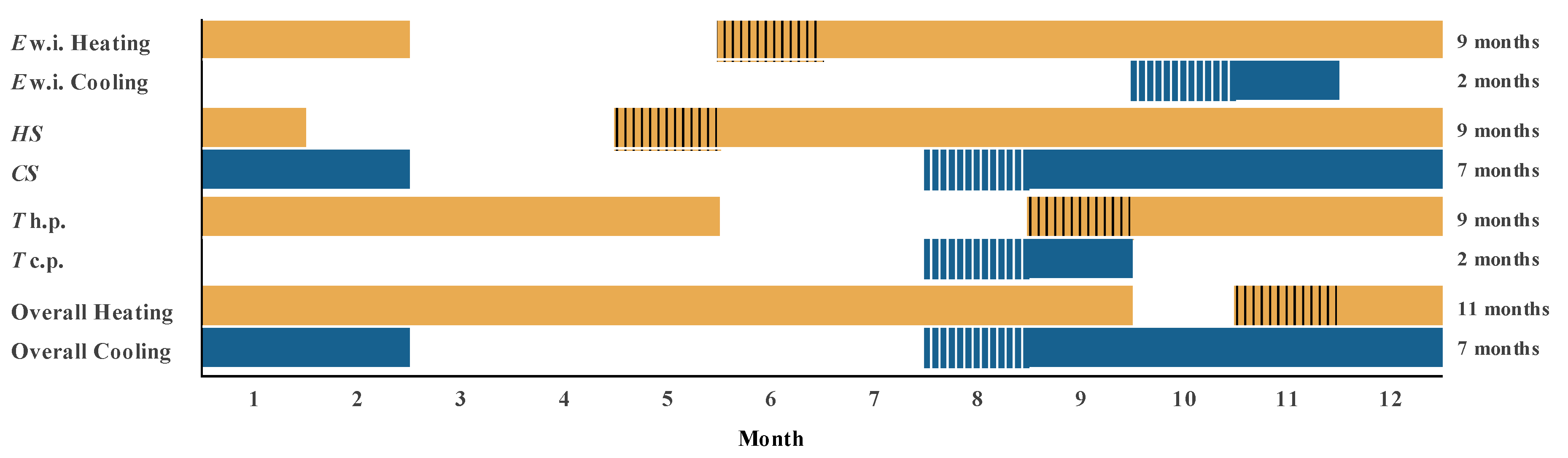
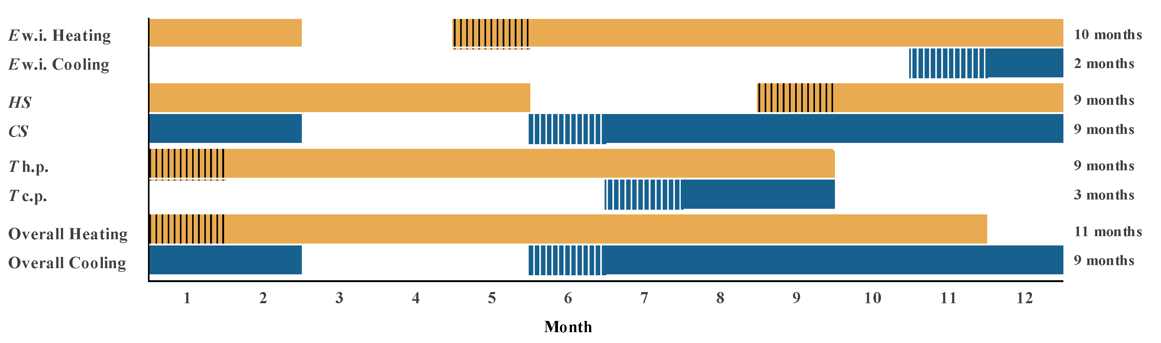
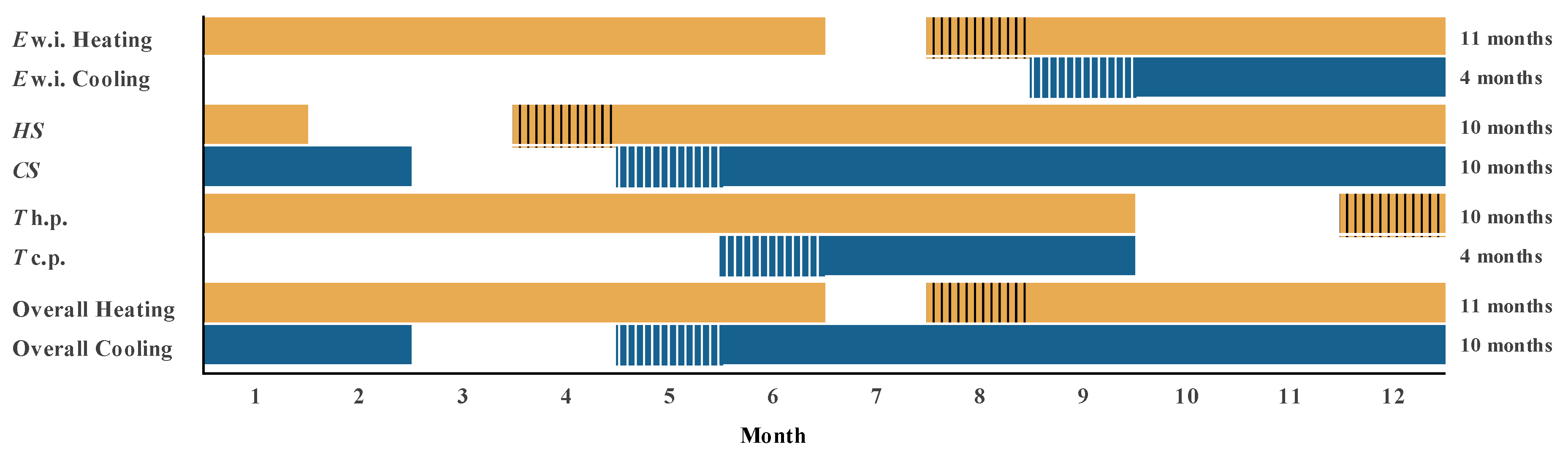
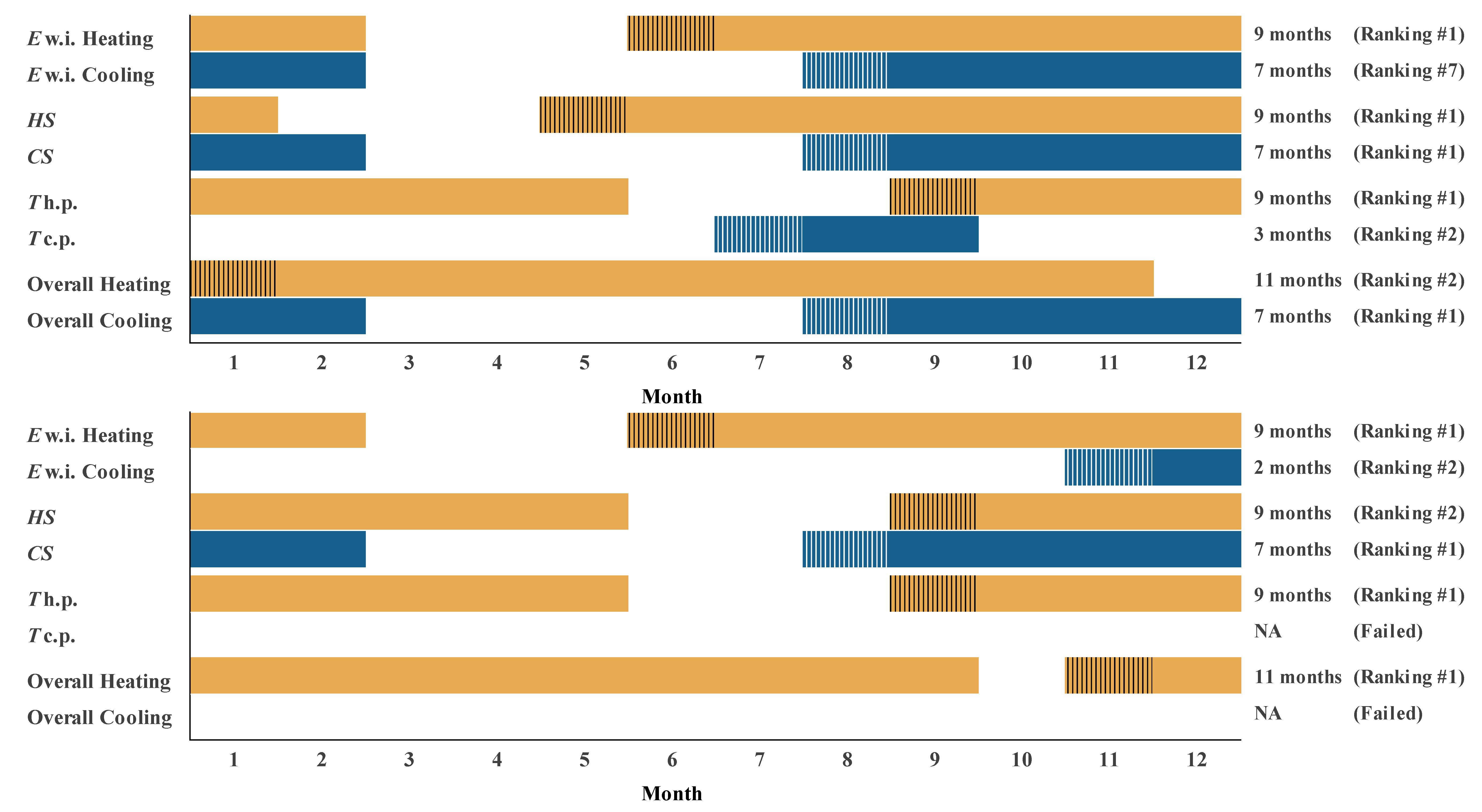
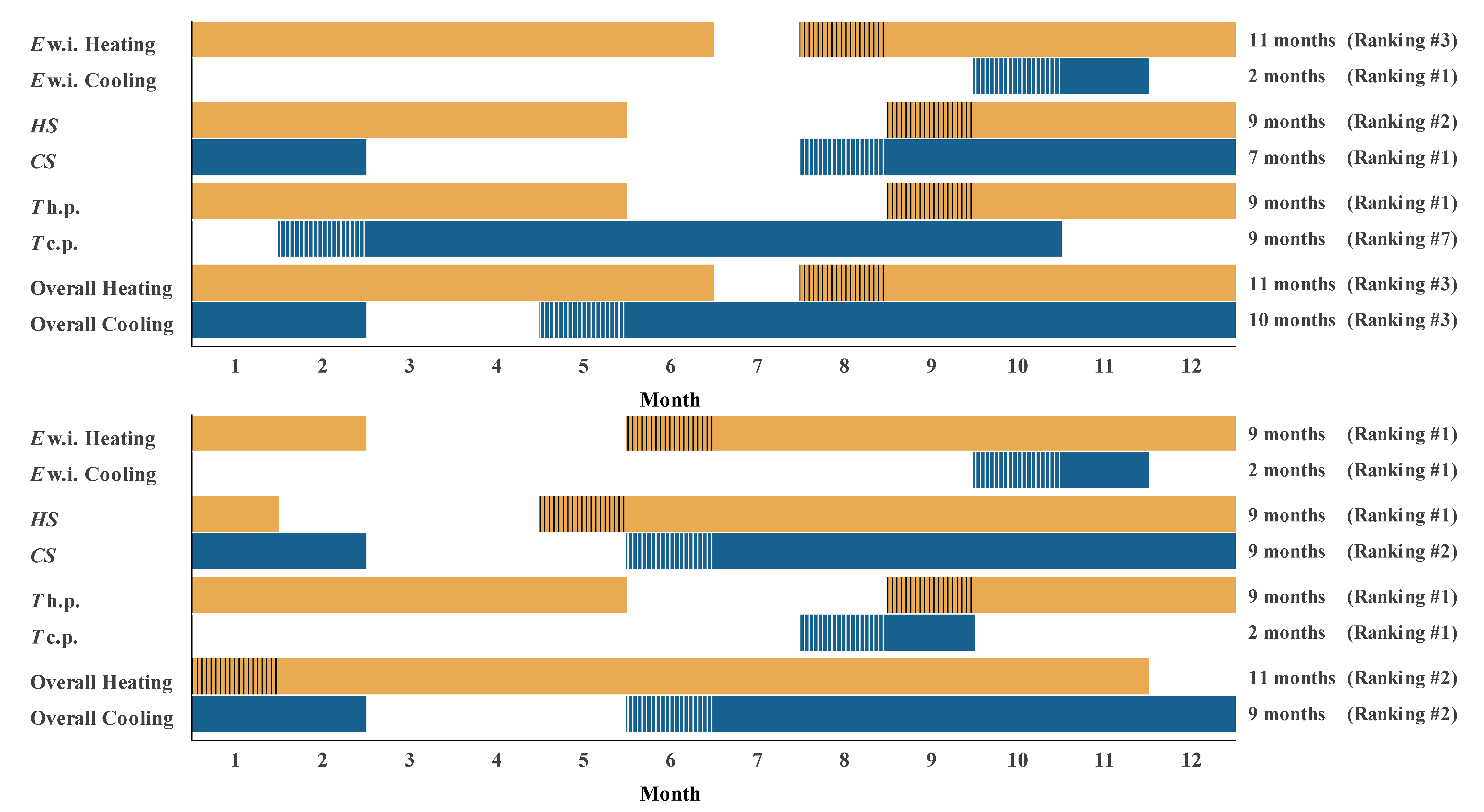
4.2. Comparison between Short-Term Heating and Cooling Energy Monitoring Performance

A graphical approach was developed to compare the best energy monitoring periods when cooling and heating energy performance was considered. The main findings from this comparison were different monthly and seasonal periods between short-term heating and cooling energy monitoring. Figure 7, Figure 8 and Figure 9 show the results from the comparison between the heating and cooling performance for short-term monitoring data from unit #602. The perpendicular line patterns on the bars indicate the starting month of the monitoring period that was determined for each coefficient. The orange and blue-colored bars represent the time periods for heating and cooling loads, respectively. The heating and cooling periods show the significant differences on the months in Figure 7 through Figure 9. For example, for the non-weather-related energy monitoring periods, the starting month of June (Summer) with 9 months were required for heating while the starting month of October (Fall) with 2 months were required for cooling (see the upper two bars in Figure 7).

The discontinued spaces where the bars are not presented on the x-axis show the months when it is not necessary to measure heating or cooling energy use performance. In other words, monitoring costs can be saved because monitoring is not needed during these months. Unfortunately, when both the heating and cooling loads’ interval data were considered, all 12 months were required to analyze all the coefficients. In addition, all 12 months were required for the heating energy use data. In other words, the orange bars do not have the common months that are not presented on the x-axis from Figure 7 through Figure 9. However, it was observed that the time periods from March to July in Figure 7 (i.e., ranking #1), from March to May in Figure 8 (i.e., ranking #2), and from March to April in Figure 9 (i.e., ranking #3) do not require monitoring systems or data loggers to be installed in order to analyze the cooling energy use data. This graphical approach is very useful to identify the months when it is unnecessary to perform short-term monitoring in order to save time and costs. In other words, the blue bars have the common months that are not presented on the x-axis from Figure 7 through Figure 9.

In addition, the graphical approach is useful to easily compare the length of the time periods required to identify the weather-independent energy use, the weather-dependent energy use, and the change-point temperatures. Typically, the length of the time period required for the cooling energy performance was shorter than the heating energy performance. Particularly, the lengths of the periods for the non-weather-related cooling load and cooling change-point temperature were much shorter. For example, the highest-ranked time periods for the weather-independent cooling load and cooling balance-point temperature were 2 months long, while the periods for the heating energy use data were 9 months long. Using the graphical approach, it was also observed that the starting months were more distributed for the heating energy use data, while the starting months for the cooling energy use data were not distributed. The starting months for the cooling slope, the cooling balance-point temperature, and the overall cooling approach were the same, or within a difference of one month.

Figure 10 and Figure 11 show the graphical approach used to compare the best short-term monitoring periods from unit #602 to evaluate if the identified short-term periods could be applied to the other residences (#301, #304, #503, and #601). The #1 and #2 ranked time periods from #602 were properly applied to search the best energy monitoring periods at #301, with the exception of the non-weather-related cooling coefficient at the ranking #7 (see the upper plot in Figure 10). The figure shows that the cooling energy use data does not need to be collected between March and June. The results were similar for unit #304. The #1 and #2 ranked time periods from unit #602 were properly applied to search the short-term energy monitoring periods at #304, with the exception of the cooling balance-point temperature and overall cooling coefficients (i.e., failed) (see the lower plot in Figure 10). The short-term monitoring periods from #602 did not work for the cooling change-point temperature coefficient and the overall cooling coefficient because the cooling balance-point temperature of 24.1 °C at #602 was significantly different from the balance-point temperature of 7.6 °C at #304.

At #503, with the exception of the cooling balance-point coefficient, the time periods in rankings #1 through #3 from #602 were properly applied to search the best monitoring periods, as shown in Figure 11 in the upper plot. The figure identifies that the month of July is not necessary when collecting heating energy use data. In residence #601, the #1 and #2 ranked time periods from #602 were able to completely describe the short-term monitoring periods (see the lower plot in Figure 11). For this case, March to May can be excluded when collecting cooling energy use data. This graphical approach is very useful for identifying the time periods when monitoring can be applicable and highlighting the unnecessary months to save time and costs. Furthermore, the graphical analysis approach from the coefficient checking method can also be useful to estimate missing heating and cooling energy use data from other residences that have similar characteristics, such as residences in a high-rise apartment building. In summary, the comparison analysis, including the graphical approach, shows the effectiveness of the coefficient checking method because the best short-term energy monitoring periods for heating and cooling loads are significantly different even though the residences have the same building characteristics. Using the statistical coefficients along with the physical meanings, the best short-term monitoring periods can be found by a specific category, such as non-weather-related and weather-related heating and cooling energy use as well as estimated occupancy, building system, and/or appliance types and schedules. Furthermore, it was observed that the best short-term monitoring periods from unit #602 were well applied to the other residences (#301, #304, #503, and #601) for both heating and cooling loads. This shows the applicability of the coefficient checking method if residences have similar building characteristics, and the change-point models provide the goodness-of-fit results for residential interval energy use data.

5. Discussion

In this paper, we presented the approaches and results from the heating coefficient checking method using interval natural gas use data. A 3PH model was used to estimate heating loads from the 49 residences of a case study high-rise residential building. Using the goodness-of-fit indices for 3PH models and the resultant cases from the previous study [25], the five residences were selected. Then, the three coefficients of the 3PH models were used to search the best periods in terms of short-term energy monitoring on non-weather-related and weather-related heating energy use. We found that 9-month periods were required to search the best short-term heating energy monitoring periods when non-weather-related and weather-related heating loads and heating change-point temperatures are considered. In addition, the 9-month to 11-month periods were needed for the analysis to apply to other case study residences. In the previous study, the short-term monitoring periods for analyzing the cooling energy performance were 2 months, 7 months, and 2 months for each cooling coefficient [25]. Between 2-month to 10-month periods of the short-term cooling energy monitoring were needed to apply the same analysis to other case study residences.

Based on the best monthly periods, the unnecessary monitoring months (i.e., when the data logger is not necessary to observe heating and/or cooling energy use performance) were also found. The graphical approach (see Figure 7 through Figure 11) effectively identified the months when it is unnecessary to perform short-term monitoring. Time and costs can be saved by not installing or stopping the monitoring systems during the unnecessary months.

However, this study showed some limitations. The analysis approach of this study should consider two factors: (1) the residences should have similar characteristics, as would be expected of residences in the multi-family residential building type, and (2) goodness-of-fit indices for residential interval energy use data, such as weekly heating energy use data, should be acceptable for the change-point models. In addition, the impact on the location of each residence was not considered. For example, the residence on the fourteenth floor will be more affected by heat gains from the solar radiation, compared to the residence on the second floor. To improve the current coefficient checking method, we will cover those limitations by developing new statistical models.

6. Conclusions

We presented the approaches and results from the heating coefficient checking method, as well as the comparison with the results from the cooling coefficient checking method in the previous study [25]. Using the statistical coefficients along with the physical meanings from the change-point models of the coefficient checking method, the best short-term monitoring periods were found by specific categories, such as non-weather-related and weather-related heating and cooling energy use. The physical meanings from the coefficients could be used to estimate occupancy, building system, and/or appliance types and schedules. This will be very helpful when an energy auditor starts the process to find specific energy-saving opportunities at residences.

In addition, we found that the best short-term monitoring periods from unit #602 were well applied to the other residences (#301, #304, #503, and #601) for both heating and cooling loads. This shows the applicability of the coefficient checking method. This would be very useful if monitoring equipment met malfunctions (i.e., missing data) at some residences in the same apartment. An energy auditor can use energy consumption data from one residence to apply to others. It was also found that the period of short-term energy monitoring can be used to effectively collect targeted data for an annual prediction.

From the comparison analysis, it was found that the best short-term energy monitoring periods for heating and cooling loads were significantly different. The differences can provide an energy auditor with the useful information to reduce time and costs by avoiding unnecessary months for installing monitoring systems for heating and/or cooling loads. Furthermore, it is noteworthy that the short-term heating energy monitoring periods were much longer than the cooling energy monitoring periods. Such a result can be caused because the heating energy use data had higher CV-RMSE values, even though the R² values of the heating energy use were actually higher than the cooling energy use. Therefore, it was observed that CV-RMSE is a more important statistical index for the coefficient checking method. For a future study, specific reasons for the period differences between heating and cooling loads will be identified. The actual time and costs saved from the coefficient checking method will also be quantified.

Even though the coefficient checking method has some limitations, the approach provides a simple evaluation using the coefficients from change-point models. As a result, the analysis approach used in this study will help enhance energy auditing processes to identify both the best heating and cooling periods for short-term monitoring, which can save time and cost by avoiding unnecessary monthly periods for collecting interval heating and/or cooling energy performance data. In addition, the detailed comparison between the heating and cooling monitoring periods will be helpful to effectively collect targeted data for energy audits and annual predictions in multi-family residential buildings.

References

1. The Ministry of Trade Industry and Energy. National Energy Basic Plan of 2019; The Ministry of Trade Industry and Energy: Sejong, Korea, 2019.
2. Martins, J.F.; Pronto, A.G.; Delgado-Gomes, V.; Sanduleac, M. Chapter 4—Smart Meters and Advanced Metering Infrastructure. In Pathways to a Smarter Power System; Taşcıkaraoğlu, A., Erdinç, O., Eds.; Academic Press: Cambridge, MA, USA, 2019; pp. 89–114. ISBN 978-0-08-102592-5. [Google Scholar]
3. Cebe, M.; Akkaya, K. Efficient certificate revocation management schemes for IoT-based advanced metering infrastructures in smart cities. Ad Hoc Netw. 2019, 92, 101801. [Google Scholar] [CrossRef]
4. Bohli, J.M.; Sorge, C.; Ugus, O. A privacy model for smart metering. In Proceedings of the 2010 IEEE International Conference on Communications Workshops, Capetown, South Africa, 23–27 May 2010; pp. 1–5. [Google Scholar]
5. Molina-Markham, A.; Shenoy, P.; Fu, K.; Cecchet, E.; Irwin, D. Private memoirs of a smart meter. In Proceedings of the BuildSys’10—Proceedings of the 2nd ACM Workshop on Embedded Sensing Systems for Energy-Efficiency in Buildings; ACM: Zurich, Switzerland, 2010; pp. 61–66. [Google Scholar]
6. Oh, S.; Haberl, J.S.; Baltazar, J.-C. Analysis methods for characterizing energy saving opportunities from home automation devices using smart meter data. Energy Build. 2020, 216, 109955. [Google Scholar] [CrossRef]
7. Mack, P. Chapter 35 - Big Data, Data Mining, and Predictive Analytics and High Performance Computing. In Renewable Energy Integration; Jones, L.E., Ed.; Academic Press: Boston, MA, USA, 2014; pp. 439–454. ISBN 978-0-12-407910-6. [Google Scholar]
8. ASHRAE. Chapter 19—Energy estimating and modeling methods. In ASHRAE Handbook—Fundamentals; ASHRAE: Atlanta, GA, USA, 2017. [Google Scholar]
9. Kissock, K.; Haberl, J.S.; Claridge, D.E. Inverse Modeling Toolkit: User’s Guide (ASHRAE Final Report for RP-1050); ASHRAE: Atlanta, GA, USA, 2001. [Google Scholar]
10. Haberl, J.S.; Sreshthaputra, A.; Claridge, D.E.; Kissock, J.K. Inverse Model Toolkit: Application and testing (RP-1050). ASHRAE Trans. 2003, 109, 435–448. [Google Scholar]
11. Pham, A.-D.; Ngo, N.-T.; Ha Truong, T.T.; Huynh, N.-T.; Truong, N.-S. Predicting energy consumption in multiple buildings using machine learning for improving energy efficiency and sustainability. J. Clean. Prod. 2020, 260, 121082. [Google Scholar] [CrossRef]
12. Fan, C.; Xiao, F.; Yan, C.; Liu, C.; Li, Z.; Wang, J. A novel methodology to explain and evaluate data-driven building energy performance models based on interpretable machine learning. Appl. Energy 2019, 235, 1551–1560. [Google Scholar] [CrossRef]
13. US DOE Home Energy Audits. Available online: https://www.energy.gov/energysaver/weatherize/home-energy-audits (accessed on 3 April 2020).
14. Gunay, B.; Shen, W.; Newsham, G.; Ashouri, A. Detection and interpretation of anomalies in building energy use through inverse modeling. Sci. Technol. Built Environ. 2019, 25, 488–503. [Google Scholar] [CrossRef]
15. Perez, K.X.; Cetin, K.; Baldea, M.; Edgar, T.F. Development and analysis of residential change-point models from smart meter data. Energy Build. 2017, 139, 351–359. [Google Scholar] [CrossRef] [Green Version]
16. Kim, K.H.; Haberl, J.S. Development of a home energy audit methodology for determining energy-efficient, cost-effective measures in existing single-family houses using an easy-to-use simulation. Build. Simul. 2015, 8, 515–528. [Google Scholar] [CrossRef]
17. Do, H.; Cetin, K.S. Evaluation of the causes and impact of outliers on residential building energy use prediction using inverse modeling. Build. Environ. 2018, 138, 194–206. [Google Scholar] [CrossRef]
18. Ali, M.T.; Mokhtar, M.; Chiesa, M.; Armstrong, P. A cooling change-point model of community-aggregate electrical load. Energy Build. 2011, 43, 28–37. [Google Scholar] [CrossRef]
19. Zhang, Y.; O’Neill, Z.; Dong, B.; Augenbroe, G. Comparisons of inverse modeling approaches for predicting building energy performance. Build. Environ. 2015, 86, 177–190. [Google Scholar] [CrossRef]
20. Wang, J.; Gao, Y.; Chen, X. A Novel Hybrid Interval Prediction Approach Based on Modified Lower Upper Bound Estimation in Combination with Multi-Objective Salp Swarm Algorithm for Short-Term Load Forecasting. Energies 2018, 11, 1561. [Google Scholar] [CrossRef] [Green Version]
21. Noussan, M.; Nastasi, B. Data Analysis of Heating Systems for Buildings—A Tool for Energy Planning, Policies and Systems Simulation. Energies 2018, 11, 233. [Google Scholar] [CrossRef] [Green Version]
22. Nugraha, G.D.; Musa, A.; Cho, J.; Park, K.; Choi, D. Lambda-Based Data Processing Architecture for Two-Level Load Forecasting in Residential Buildings. Energies 2018, 11, 772. [Google Scholar] [CrossRef] [Green Version]
23. Abushakra, B.; Paulus, M.T. An hourly hybrid multi-variate change-point inverse model using short-term monitored data for annual prediction of building energy performance, part I: Background (1404-RP). Sci. Technol. Built Environ. 2016, 22, 976–983. [Google Scholar] [CrossRef]
24. Singh, V.; Reddy, T.A.; Abushakra, B. Predicting annual energy use in buildings using short-term monitoring: The dry-bulb temperature analysis (DBTA) method. ASHRAE Trans. 2014, 120, 397–405. [Google Scholar]
25. Oh, S.; Kim, K.H. Change-point modeling analysis for multi-residential buildings: A case study in South Korea. Energy Build. 2020, 214, 109901. [Google Scholar] [CrossRef]
26. Korean Meteorological Administration Korean Meteorological Data Portal. Available online: https://data.kma.go.kr (accessed on 19 March 2020).
27. Lee, K.; Baek, H.-J.; Cho, C. The estimation of base temperature for heating and cooling degree-days for South Korea. J. Appl. Meteorol. Climatol. 2014, 53, 300–309. [Google Scholar] [CrossRef]
28. Kissock, J.K.; Haberl, J.S.; Claridge, D.E. Inverse Modeling Toolkit: Numerical algorithms (RP-1050). ASHRAE Trans. 2003, 109, 425–434. [Google Scholar]
29. Prahl, D.; Beach, R. Analysis of Pre-Retrofit Building and Utility Data; National Renewable Energy Lab (NREL): Golden, CO, USA, 2014.
30. ASHRAE. ASHRAE Guideline 14-2014; ASHRAE: Atlanta, GA, USA, 2014. [Google Scholar]
31. Kim, K.H.; Haberl, J.S. Development of methodology for calibrated simulation in single-family residential buildings using three-parameter change-point regression model. Energy Build. 2015, 99, 140–152. [Google Scholar] [CrossRef]
32. Sever, F.; Kissock, K.; Brown, D.; Mulqueen, S. Estimating industrial building energy savings using inverse simulation. ASHRAE Trans. 2011, 117, 348–355. [Google Scholar]
Figure 1. Overall procedures.
Energies 13 03189 g001
Figure 2. Floor plan of the case study residence in the high-rise apartment.
Energies 13 03189 g002
Figure 3. Procedures used for the coefficient checking method for the heating energy use data.
Energies 13 03189 g003
Figure 4. Non-weather-related coefficient ( E w . i . ) differences (%) from the baseline coefficient.
Energies 13 03189 g004
Figure 5. Heating slope coefficient ( H S ) differences (%) from the baseline coefficient.
Energies 13 03189 g005
Figure 6. Heating balance-point temperature differences (%) from the baseline coefficient.
Energies 13 03189 g006
Figure 7. Comparison of the best periods from ranking #1 for unit #602.
Energies 13 03189 g007
Figure 8. Comparison of the best periods from ranking #2 for unit #602.
Energies 13 03189 g008
Figure 9. Comparison of the best periods from ranking #3 for unit #602.
Energies 13 03189 g009
Figure 10. Comparison of the best periods for unit #301 (upper) and unit #304 (lower).
Energies 13 03189 g010
Figure 11. Comparison of the best periods for unit #503 (upper) and unit #601 (lower).
Energies 13 03189 g011