Total Cost of Ownership Model and Significant Cost Parameters for the Design of Electric Bus Systems


1
Department of Electrical Engineering, Chalmers University of Technology, SE-412 96 Gothenburg, Sweden
2
Blekinge Institute of Technology, TISU, SE-37179 Karlskrona, Sweden
3
Rise Research Institutes of Sweden, Lindholmspiren 3A, SE-41756 Gothenburg, Sweden
*
Author to whom correspondence should be addressed.
Energies 2020, 13(12), 3262; https://0-doi-org.brum.beds.ac.uk/10.3390/en13123262
Submission received: 14 May 2020
/
Revised: 10 June 2020
/
Accepted: 17 June 2020
/
Published: 24 June 2020
(This article belongs to the Special Issue Electric Systems for Transportation)
Abstract
:Without experiences of electric buses, public transport authorities and bus operators have faced questions about how to implement them in a cost-effective way. Simple cost modelling cannot show how costs for different types of electric buses differ between different routes and timetables. Tools (e.g., HASTUS, PtMS, and optibus) which can analyse such details are complicated, time consuming to use, and provide insufficient insights into the mechanisms that influence the cost. This paper therefore proposes a method for how to calculate total cost of ownership, for different types of electric buses, in a way which can predict how the cost varies based on route and timetable. The method excludes factors which cause minor cost variations in an almost random manor, in order to better show the fundamental mechanisms influencing different costs. The method will help in finding ways to reduce the cost and help to define a few cases which deserve a deep analysis with more complete tools. Testing of the method in a Swedish context showed that the results are in line with other theoretical and practical studies, and how the total cost of ownership can vary depending on the variables.

1. Introduction
Electric cars and buses has been proposed by several studies and authorities as a long-term solution for the sustainable development of transport systems, mainly because of their high efficiency, very low emissions when being driven, low noise levels, and the possibility of using renewable sources for their electricity (e.g., [1,2,3]). Several predictions estimate that electric vehicles will dominate the sales within the next decade (e.g., BloombergNEF believe electric cars will dominate after 2036, and electric buses after 2030 [4] and IEA believe that sales of EVs will be 70% in 2030 [5]) as the price for batteries is likely to decrease and governmental incentives are likely to increase to support such development of the transport sector. A commonality in countries with incentives to tackle climate-change issues related to transport (e.g., taxes on fossil fuels) is that the current approximately 50% higher purchase price for electric cars can be compensated with a much lower price for electricity per km. For example, in Sweden in 2019, the VW e-Golf had a lower total cost of ownership (TCO) after three years (accumulated TCO after five years) than a comparable VW Golf powered by fossil fuels with a mileage of 15 km per year [6]. However, TCO is different for cars and buses, because buses usually have a higher use rate and longer mileage (a bus is normally driven 4–8 times more kilometres than a car). However, bus operators have been reluctant to use electric buses in their operations, mainly because of higher purchase costs and a lack of knowledge regarding how to design, operate, and maintain electric bus systems [7]. Contradictory, a study by Borén [1] summarized several studies about electric buses in Sweden and showed that electric buses can reduce the total cost of ownership for bus operators by more than 10% over a 10-year period, as well as societal costs due to low life-cycle emissions and noise levels when compared to buses powered by diesel and gas (methane). This depends on country-specific conditions, and a recent study in Texas (USA) show that electric buses can become cost competitive in about 5 years [8], while a study in India show that electric buses can be cost competitive within 25 years [9], and a study in Turkey showed that electric buses have twice as long pay-back time (almost six years) than diesel buses [10]. Since the greenhouse gas emissions from electricity production varies a lot from country to country, electric buses could actually emit more greenhouse gas emissions in total than diesel buses if the electricity used for electric buses is produced with high carbon intensity, e.g., electricity mix in Malta, Poland, Latvia, and Estonia [11]. Some of these emissions can be linked to the production of batteries if there is an extensive use of energy that stem from fossil resources (e.g., oil, coal, and natural gas) [12]. This can, however, be compensated by subscriptions or shares in (or establishment of) new facilities for electricity produced from renewable sources. However, the efforts to reduce climate change and other sustainability impacts cannot only address the transport system, leaving the electricity sector to continue to use fossil fuels. The increase in renewable electricity production and a decline in the cost of it will likely make it possible to achieve a rather quick transition towards sustainable electricity production. Electric buses will then have a minor contribution to climate change and other emissions.
While there can be many environmental and health-related advantages to switch from fossil-fuelled buses to electric, it is important to make that transition relatively easy and cost-efficient to get bus-operators (and taxpayers in the long run) onboard. There have been analyses completed and models/tools designed that focus on charging systems’ design and costs [13], location of charging infrastructure [14], costs and sustainability for electric buses [1], life-cycle environmental impacts [12], and procurement processes [15]. There are also several commercial tools (e.g., HASTUS, PtMS, and Optibus [16,17,18]) used by public transport authorities and bus operators for the calculation of costs related to bus traffic, but without the integration of electric bus systems. Based on that, the authors of this paper have identified a need to focus on modelling and analysis of the total cost of operating electric buses that are charged either at the bus depot or/and along the bus route. What complicates the search for the most cost-effective electric bus system is that the cost of different types of bus systems changes with route properties and timetables.
1.1. Different Types of Electric Buses
Electric buses have a very low operating cost compared with conventional buses, but a higher investment cost of the battery and chargers, and sometimes additional cost of the driver waiting during charging and for extra buses required due to the charging time. It is not possible to minimize all these cost at the same time, so there is a need to find a cost-effective compromise, which depend on the timetable and bus route properties, and that is why several different charging strategies are relevant for analysis.
Charging at the end stops means that the buses can have smaller batteries than buses charged at a bus depot, as they can charge after each trip. This can be cost effective as long as there are many departures per hour, allowing the chargers to be frequently used. The chargers are used very little if the bus route has low bus traffic density, and a low utilization of the chargers increases the cost per trip kilometre. One of the drawbacks of charging at the end stop after each trip is that there is a need for extra buses to have time to charge.
The operators want to minimize the number of buses for a bus line since the investment in buses is a major cost driver. That is why the second charging strategy in this paper, end-stop charging off-peak, is included. All buses then drive during peak times without charging. Between the morning and afternoon peak times, typically 09:00 to 14:00, all buses are not needed in traffic, so then they can charge. This will reduce the number of buses, but it will also require bigger batteries onboard since the buses need to be able to drive for about three hours without charging. It is not obvious which timetables and bus routes that could make one or the other charging strategy more cost effective.
1.2. Aim of the Paper
This paper addresses the needs and challenges described earlier. There is not one solution of electric buses which can always be assumed to be the best, and there are many factors which influence when a certain type of electric bus is cost effective or not. The goal of this paper is to present a cost model which can model the main mechanisms that influence the costs of electric buses when different routes and timetables are compared. Besides calculating costs, the model can also help explain why and how different factors influence the costs, and thus make it easier to find ways to reduce costs. The model can be used for many types of electric buses, but in this paper, it is only used to analyse electric buses mainly charged at the end stops. The costs for electric buses are also compared with buses powered by biofuels (gas and diesel) to find which type of routes of electric buses with end-stop charging are most cost effective.
1.3. Limitations
To better serve the purpose of identifying the underlying mechanisms, rather than giving an exact conclusion of a specific route, several simplifications are made. For example, the Total Cost of Ownership (TCO) model can calculate the cost of a non-integer number of buses. Such simplifications make it much easier to identify some general trends in cost changes and explain what causes them, but they also mean that the model is not intended to use when conducting the final and detailed cost analysis on a route. Rather, its purpose is to help determine which types of buses are interesting to investigate for a specific route, while the final analysis should be made with a more detailed bus-planning and cost analysis tool. The focus of the paper is to present the cost model, while analysis of bus routes is included only as examples of how the model can be used. The cost results presented should therefore not be seen as representative for all bus routes. The parameter values used in the examples are for a Swedish context and may need to be changed when analysing other bus routes.
The paper analyses the two charging strategies for electric buses: end-stop charging—when they are charged at the end stops on a route (included in the opportunity charging concept); and end-stop off-peak charging—buses charged at the end stops for the whole day except during the peak hours. The buses are also charged in the depot during night in order to be fully charged when they start operations. Both the electric bus charging strategies are compared with buses powered by biomethane or Hydrogenated Vegetable Oil (HVO), which is a biodiesel that can be used as a drop-in fuel in conventional diesel engines. In Sweden almost all buses run on biofuels, so we have not included diesel buses in the comparisons in Section 5. Diesel buses will have exactly the same costs as HVO buses, excluding the fact that the price of diesel fuel differs to that of HVO.
1.4. Structure of the Paper
Section 2 explains what the model calculates and in what steps. First, the method and core assumptions are presented. The modelling starts from a formula for calculating the TCO, and that formula is used to identify which intermediate variables influences the total cost. In Section 3, the parameters which are used to describe the bus route and timetable are presented, as are the basic cost parameters. Section 4 then shows how the intermediate variables can be calculated from the parameters for the route and timetable. The explanations of the charging strategies, and some assumptions related to them, are also found in Section 4, as deriving the model is closely linked to the explanation of the charging strategies. In Section 5, an analysis of end-stop-charged buses is presented, with the aim of explaining the mechanisms which influence the cost of running a route and how different types of routes and timetables influences their TCO. This analysis is intended to demonstrate what the model can be used for, rather than providing cost results which can be used for any bus route. Finally, Section 6 summaries the main findings in the paper, followed by a critical assessment and comparison with other studies. The very last part then focuses on how the paper contributes to the research community, and on recommended further work.
2. Model for Total Cost of Ownership
2.1. Method
The TCO model is built in Matlab [19], which is a software that integrates computation, visualization, and programming in an environment where problems and solutions are expressed in mathematical notation. The model is based on a direct step by step calculation of the results starting only from the parameters describing the route and the timetable, as well as the bus and cost parameters. This direct calculation method is possible since the calculations have been broken down in steps which can calculate their respective outputs while only knowing input parameters and intermediate results calculated in previous steps. All the equations have been solved analytically before creating the TCO calculation program. Furthermore, the order of the calculations has been carefully selected so that there is no need to feed results back to previous calculation steps, avoiding the need for numerical solvers in the program. This leads to a quick program that is easy to follow, despite having a significant number of steps in the calculations.
Another key part of the method is to avoid calculating more details than needed. This is done by, as far as possible, directly calculate energies and bus time for the whole fleet of buses, rather than for each individual bus. Furthermore, the smallest step in the calculation of a whole day of bus traffic is the single bus trip. No finer time step is analysed, which means that there is no need to simulate the individual buses, which also ensures a quick calculation.
Since the purpose is to find and model the general mechanisms which influence the TCO, it is important to only include the important factors and exclude all minor effects that will mainly show up as a noise in the calculation of the cost. The way we do this is to start from the end result, the TCO equation, and derive the model backwards from there. This ensures that we only include things that can influence the TCO, while all other aspects of buses will automatically be excluded. Later in this section, we also discuss how the model avoids factors which can cause small variations up and down in cost when timetable and route parameters only slightly change. These are therefore seen as noise, which is not a part of the overall trend in the cost variations.
2.2. Output of the Total Cost of Ownership Model
In this paper, the TCO will be presented either as a total cost per year for the investigated route, or as the route’s total cost per trip kilometre. The cost per trip kilometre is the TCO per year divided by the total distance all the buses drive in service. Cost of driving outside the timetable, such as driving to or from the depot and driving between different routes, is included in both cost measures, but when the specific cost per km is calculated, the cost is only divided on the kilometers driven during the trips. This is important since driving to and from the depot adds nothing to the value of the route, while it adds to the cost of operating the route.
The total cost per year is obviously a good measure of how cost effective a certain bus type is for a specific route. However, it is not so useful for general conclusions and comparisons of different bus routes which have very different bus traffic density and different lengths. Then, the total yearly cost will be very different and does not clearly illustrate which system is more cost-effective. When comparing different routes and different bus traffic volume, it is often better to compare cost per trip (km) instead. Even if bus lines can have total yearly costs which are different by an order of magnitude, a comparison of their cost per trip (km) will be revealing. The difference in costs per trip (km) then indicates why one of the routes is more cost-effective than the other.
2.3. Parameters Used to Determine Total Cost of Ownership
The TCO is calculated as the sum of operating cost and investment-related costs. In this model, the operating cost is the sum of driver cost, energy cost, maintenance and insurance and electric grid fees. The cost of the investment is determined from the depreciation of the chargers, batteries and buses. The final calculation steps of the TCO are shown in Figure 1.
There are, of course, other costs for a route, such as the cost of depots (excluding chargers), ticket systems, etc. In this analysis it is assumed that such costs are the same for all the investigated bus types and therefore will not be important when comparing different bus types with each other. However, when cost differences between the alternatives are small, minor variations in these other costs can very well be what tips the scale in favour of one bus type or another, and that is why a final decision on what type of buses to use for a route should always be conducted based on a detailed bus-planning and cost analysis tool.
To determine these seven costs, the model use nine intermediate variables which are calculated for the analysed routes and timetables. These are:
- Driver time per year;
- Energy use per year;
- Total driven distance per year;
- Trip distance per year;
- Number of places with chargers (i.e., number of grid connections);
- Total combined power of all chargers;
- Number of chargers;
- Number of buses;
- Bus battery size.
These nine variables, together with eight cost parameters, determine the seven parts that make up the TCO. The TCO per year is the sum of the seven costs, and the TCO per trip kilometre is the TCO per year divided by the number of trip kilometres per year.
2.4. Simplifications Aimed to Find General Trends Rather than Route-Specific Results
There are some costs which vary only in steps, and these steps can make it difficult to see the general trend in the costs. For example, when the headway is varied, the number of buses needed for a route changes in steps of one. The exact headway at which the number of buses changes is not necessarily the same for the compared charging strategies. Comparing two types of buses, it may sometimes look as if one is more cost effective than the other, but with just a slight adjustment of the headway, the result can be the opposite. To avoid this, the cost model is defined to calculate as if it is possible to buy a non-integer number of buses, and by extension, a non-integer number of depot chargers. Normally several routes are driven by the same operator, and then the possibility to use a non-integer number of buses for a route is even more reasonable since buses and drivers can be shared between different routes, making it possible to plan the bus schedules so that buses can operate on several routes.
The number of end-stop chargers are, however, an integer in the model, as the step in the number of chargers will be much more important for the cost effectiveness of the different charging strategies. End-stop chargers are sometimes less well-utilized than depot chargers, and it is important that the model includes that effect, as it is a reason why the TCO for end-stop charging significantly varies between different routes. Furthermore, end-stop chargers can only support the routes that use the bus stop at which they are placed and can therefore not be shared as easily between routes as the buses can.
When planning bus schedules for a route, there is often a need for buses to be inactive and wait for the next departure. The need for such waiting time can vary in a very random way with changes in route properties and timetables. To avoid such “noise” influences on the TCO calculations, the TCO model does not create real bus schedules. Instead, the model just estimates the total number of buses needed in traffic, how many will be driving to and from the depot, and how many will be charging at different times during the day. This simplification is a feature and not a bug, since it allows for a clearer illustration of the system effects when analysing the total amount of buses occupied by different tasks rather than focusing on analysing the buses individually.
Another simplification is that the model does not keep track of the State of Charge (SoC) of individual batteries, but instead, the SoC of the buses are ensured by a few conditions regarding the size of the required batteries, and by determining how much charging is required in total to achieve energy balance of the fleet over the day. To allow for this simplification, the model assumes that the batteries are sized to handle some worst-case energy use that individual buses can experience between charges. Optimizing the battery size can further reduce costs, but this is not included in this version of the cost model.
2.5. Cost of Conventional Combustion Engine Buses
The TCO model is mainly developed to analyse electric buses, but it can also analyse conventional buses since they are less complex. As there is no need for conventional buses to be fuelled during the day, they only need to meet the requirement of driving their designated amount and the minimum number of trips to and from the depot. They need no extra time to charge or extra time to drive to and from the depot, as may be needed by electric buses. The TCO for them is calculated using the same formula, but with slightly different cost parameters, as shown in Table 1. Rather than calculating the volume of fuel consumed, the cost of the conventional buses fuel is calculated from required traction energy, the fuel cost per litre and the average fuel efficiency of the powertrain.
3. Model Input Parameters and Variables
The TCO model has many input variables which we use to describe the route and the timetable. Several of these are, later in this paper, varied to analyse how they influence the TCO. The parameters are factors which we do not vary in this analysis, but they are still needed to determine the TCO. The parameters describe important values which influence the cost of buses, batteries, chargers, drivers, and the electricity grid.
3.1. Route Variables
We do not need to know all details of the route but must know any property which influences the nine TCO variables. In this TCO model we selected to base the route description on the time it takes to drive a trip rather than how long the route is, since the required number of buses and driver time are both directly determined by the time required, rather than the distance driven. The route distance is also an input parameter, but most calculations are made based on analysing time. Then, only a few results are translated into driven distance when it is needed to calculate the TCO variables. The route properties are independent of the used timetable.
The main route variable is the net time it takes to drive one trip, which can vary over the day. In our model, we have different trip times in the off-peak period (), in the peak period (), and during the evening (). We also need to know the time to drive from the depot to the route or back from the end stop to the depot (). For simplicity reasons, we assume it to be the same time for both end stops. This is often not the case, but the given value can then be the average time for the two end stops. To determine the driven distance, we also need parameters for the trip distance (), and the distance from depot to the route’s end stops (). If needed, the trip length and net trip time can be used to calculate the average speed of the bus.
3.2. Timetable Variables
In this cost model, we have assumed that the route and timetable are identical in both directions. A simple way of describing the timetable is shown in Figure 2. It shows a generic timetable description as a curve showing the number of departures per hour from the end stops and its variation during the day. In the diagram we can see that the timetable can be described by seven time-dependent variables and three variables for number of departures per hour. By changing these 10 variable values, the timetable can be altered in our TCO analysis. Since the buses often run into the night, beyond midnight, the calculation uses time values beyond 24 h, as this simplifies the calculations. In Figure 2, the last bus departs from the end stop at 01:00 in the night, and this is coded as 25.0 h in our model.
In addition to the variables in Figure 2, there are also variables to define the layover time needed off-peak (), during peak times (), and in the evening (). The layover time is the time between when the bus arrives at the end stop from one trip, and the time it departs for the return trip. The layover time is mainly used as a buffer time so that a delayed incoming bus shall still mostly be able to depart on time on its next trip. The layover time can also provide some breaks for the driver between trips.
Instead of defining different timetables for the different types of days (weekdays, weekends, holidays etc.) the total traffic during a whole year is instead calculated as the defined typical day, multiplied with the number of effective traffic days which give an estimate of the total yearly traffic. In this paper we use .
3.3. Bus, Driver and Battery Parameters
In this section, the parameters used to determine the cost of buses, driver, and batteries are described. In the examples in this paper, we assume 12 m buses, and they have the values given in Table 1. The different size of batteries for the two types of electric buses depends on different charging strategies. Why different battery sizes are used depends on the longest time a bus can be in traffic without charging, and this will be explained more in Section 4.1. A conservative estimation of battery cost has been used. The battery price is assumed to be constant, so it is the same after seven years when the batteries are replaced. The residual battery value after seven years has also been set to zero. Table 1 shows parameter values which are relevant for Sweden 2019, mainly based on data from pilot projects. The parameter values are included to allow the reader to check and interpret the numeric results in this paper. It shall, however, be noted that development of electric buses is rapid, and the production volumes are growing fast; therefore, these parameter values can change and should not be seen as generally applicable.
For all the buses, the average power during the trip has been assumed to be 25 kW, which is based on measured energy consumption of electric buses in Sweden. It includes auxiliary loads, heating and cooling, and is a typical average value over the year. The effect that the worst-case consumption will be higher has to be considered when sizing the batteries. The economic life of the bus (depreciation period) has been set to 10 years, while the batteries have been assumed to last seven years. In the near future, batteries will most likely last 10 years, but the first generation of bus batteries may live a little shorter.
The driver wage is set to 300 SEK/h, and the driver schedules are assumed to be planned so that 90% of the driver’s time can be used to drive the bus and wait during layover time or wait during charging. This means that the effective driver cost will be 333 SEK/h that there is a driver in the bus. It is also assumed that the driver must be paid during the time the bus charge at end stops, but not when charging at the depot.
3.4. Electric Grid Parameters
There is a need to invest in one grid connection at each charger location, irrespective of how many chargers are in the same location. It is assumed that the chargers will require so much power from the grid that one new transformer or substation will have to be built for each charger location, including some new distribution lines. The cost of a new substation will depend on the total power of all the chargers in that location. The initial cost of building a substation is set to 1 Million (M) SEK and the total cost includes an additional 1000 SEK/kW. This means that a 500-kW substation will cost SEK 1.5 M SEK and a 2 MW substation 3 MSEK. These cost levels are based on dialogue with the local electric utility company in Gothenburg, Sweden, and assume that end-stop chargers are normally not built in the city centre where cost is often much higher. When calculating the depreciation of the grid investment, the economic life for the substations and grid connection has been set to 20 years.
There is also an annual fee for using the grid. This can be very different in different regions, and in this paper, it includes one fixed annual fee per substation of 5000 SEK per year plus an annual fee depending on the installed peak power of the chargers, which is 500 SEK/kW per year.
3.5. Charger Parameters
The chargers are assumed to have a base cost of 5000 SEK per charger plus a size-dependent cost of 3000 SEK/kW. The low base cost means that the cost is almost only proportional to the total installed power of the chargers. The charger depreciation is calculated using an economic life of 10 years. This is similar to a normal contract period with a bus operator in Sweden. These cost levels are based on data from pilot projects and estimates how that cost will be reduced when building many new bus chargers at once for a contract with many bus lines. The cost has also been found to be consistent with the cost of high-power charges for electric cars, which are based on the same technology.
The assumed charger power is 300 kW for the end-stop-charged buses, and is 11 kW per bus for the night chargers for buses with 100 kWh battery and 22 kW for buses with 200 kWh battery.
There is also the factor of how much of the layover time which, on average over several trips, can be used for charging at end-stop chargers (), and in this paper it is assumed to be 50%. Since the layover time is required to avoid delays, there are situations in which there will be some trips which are delayed so that there is no layover time to charge. However, the bus batteries are big enough so that one missed charge is not be a problem as long as the bus later during the day can compensate for that missed charging. That is a reason why it is assumed that some of the layover time may, on average, be used for charging.
3.6. Other Parameters
The TCO calculation also requires some other parameters. The interest rate is used to calculate the capital cost of the investments and it has been set to 3%. This is a low interest rate, but a city or government can often borrow at such low rate.
4. Calculating TCO Input Variables from Timetable and Bus Route Parameters
Figure 1 shows the nine variables needed to calculate the TCO of the buses. However, these in turn have to be calculated from the route and timetable, and this section shows the steps in which this is done. In Figure 3, the main steps are shown, and they are then described in the following sections.
4.1. Battery Size and Need to Charge during the Day
Depending on charging strategy, the buses will need to have different battery sizes. The size of the battery must be chosen to meet several requirements. The battery must have enough capacity (kWh) to supply the energy needed for the most demanding bus schedule and should also have some margin to handle disturbances, which may sometimes lead to a shortened or a completely missed charging.
Another size-related criterion is that the battery must have enough capacity to be able to deliver the necessary traction power and to handle the charger power. It is not possible to have a very small battery and discharge or charge at very high power. The fact that batteries in buses with end-stop charging must be capable of charging at high power is a reason for why they are assumed to be more expensive per kWh of stored energy. The higher cost is due to the battery cells being more expensive per kWh when they are optimized for high charging power and the battery system needing a more effective cooling system.
Finally, the battery must not wear out to quickly, and have margin so that it can still meet all the requirements for energy and power also when the battery has aged. Typically, the capacity of the battery is reduced by up to 20% when it reaches its end of life, but the maximum discharge and charge power will also be reduced when the battery ages and, as such, this also needs to be included when deciding the battery size for a bus.
For the end-stop-charged buses, the charge power and number of charge cycles will be the critical factors, and therefore it is assumed that a 100-kWh power-optimized battery is required, despite the fact that a trip typically only requires 25 kWh if it is one hour long.
For the buses which use end-stop charging but only off-peak, a 200-kWh power-optimized battery has been assumed. The peak traffic periods are up to about three hour long which requires about 75 kWh of energy.
The battery size could be optimized for each route and timetable, but it is deemed likely that the market will settle on a few battery sizes as this simplifies moving buses between different contracts and the offers possibility for the buses to have a second life if a contract is not renewed. Therefore, it is not likely that buses will be optimized for the route they operate on, rather, there will be a few standard battery sizes which the operator selects from. The optimal sizing of a battery is a very complex task and is not included in this paper.
4.2. Determining the Number of Buses Needed to Drive the Trips
The number of buses needed is calculated in two steps. First, the number of buses required to drive the trips are calculated. This will be determined by the highest number of buses in traffic during the peak periods, and it will be equal to the number of conventional buses required. After that, there is a calculation of how many extra buses are needed in order to have time to charge electric buses. This number can be zero or larger, depending on the timetable and charging strategy. The number of extra buses is calculated in the next section.
We start by looking in detail at each bus needed to drive the trips from one of the two end stops, and later we derive the formulas needed to calculate the number of buses from the detailed analysis. The use of the buses is illustrated in Figure 4. There, we can see that bus 1 starts the first trip at time according to the timetable, and before that, it has used some time driving from the depot to the start of the route, illustrated by the light blue bar. bus 1 drive the first trip during the time shown by the green bar, and there is a need for layover time at the end of it. One headway time after bus 1, bus 2 starts the second trip, followed by bus 3 and 4 after each additional headway time. Thus, the number of buses initially increases by one bus for each headway time that passes. The increase in number of buses stops after the gross trip time, because at this point, the buses which have been driving the route in the other direction have arrived and had their layover time, and they are ready to drive the next trip as a return trip. Therefore, after the gross trip time, the number of buses in traffic does not need to be increased as long as the headway is constant. Figure 4 shows that the buses alternate driving the route in both directions, as indicated by the green and blue bars.
The headway is reduced during the morning rush hours after some time in the early morning. There are no longer enough of buses returning from earlier trips to start all the trips. If the headway during rush hour is half of the headway during the early morning, the number of buses will need to increase, as shown in Figure 5, in which the morning rush hours starts at 06:00 and ends at 09:00. Note that these times show when the headway changes for the departures from the end stop. Further down the line, the reduced headway will occur later, as it takes some time for the buses to drive from the end stop. Just like at the start of the traffic in early morning, there will be a need for more buses at the beginning of the rush hours. In this example, every second bus starting a trip from the end stop must be an additional bus coming from the depot. As before, the number of buses increases, now by one every second headway time. This continues for a time equal to the gross trip time when enough buses arrive from the other direction of the route.
At the end of the rush hour, when the headway is increased, not all buses arriving from the other direction are needed, so after the end of the morning peak, some of the buses are taken out of traffic and return to the depot.
Based on the previous analysis, we can determine the number of buses needed in traffic during the whole day. Note that we previously showed which bus is driving which trip, so that each row in the diagram is the schedule for one particular bus during the day. In the following analysis, we will derive a diagram that looks very similar, but it only shows how many buses are occupied by different activities during the day, without showing which bus is doing what. This way, we can simplify the analysis a lot, and do not need to plan the schedules of the buses. On the other hand, this analysis cannot capture all the small details involved in planning bus schedules, and some of the details in the scheduling are instead included as factors to take into account that it is not possible to plan bus schedules completely without slack for the bus and drivers.
The number of buses required for the traffic will vary during the day, as shown in the diagram in Figure 6, and it is derived from the timetable and data regarding driving time and layover time for the route. We will later use this diagram to determine how much time is available for charging during different parts of the day. Right now, we only need to know the number of buses required to drive during the off-peak period, during the peak times and in the evening. Note that despite being similar to the timetable diagram in Figure 2, this shows the total number of busses in traffic, while the timetable diagram shows the frequency of departures. How many buses are needed will not only depend on the timetable but also on the time it takes to drive the route. A short route of course needs fewer buses to follow a certain timetable than a longer bus route with the same timetable.
The number of buses required for driving all trips during peak traffic:
where the gross trip time in the peak is:
As stated earlier we do not round this off to the nearest higher integer, but instead analyse the TCO based on a non-integer number of buses. This way of calculating the number of buses assumes that the gross trip time is shorter than the peak periods. That is the case for most routes in cities, at least in Sweden, since the peak period in the morning and afternoon are typically 2 h and 3 h or more, respectively, while very few routes have more than a 2-h trip time. The number of buses in traffic during the midday off-peak period can be calculated in the same way:
where the gross trip time off-peak is:
Finally, the number of buses in traffic during the evening is:
where the evening gross trip time is:
4.3. Determining the Number of Extra Buses to Provide Time to Charge
We now know the number of base buses needed to drive the traffic, but there is also a need to provide time for the buses to charge, and that may require extra buses. Thus, in this section, we determine the number of extra buses needed for charging. Note that the biogas buses and HVO buses do not require any extra buses beyond the base buses. Besides night charging, which is assumed to allow the buses to start each day fully charged, we divide the charging in three categories to make it easier to build and understand the model. The categories of daily charging are:
4.3.1. Extra Buses for End-Stop Charging for a Whole Day (EndStop1)
With this charging strategy, the buses are charged after each trip, and it is called EndStop1 in the calculations. The energy charged equals the energy used during the last trip, which means that the buses always starts each trip with the same battery state-of-charge. The number of extra buses required is determined by calculating how much time is required to charge the bus after each trip. The calculation is made for the peak periods, as that is when the greatest number of buses will be charging simultaneously. The amount of energy that the bus must charge at each end stop is:
The charge time is:
This charge time can be used to calculate a factor for how many buses need to be charging per bus in traffic:
Now the number of extra buses required to allow for charging at end stops during peak times can be determined:
The number of buses charging off-peak and in the evening can be calculated with Equations (7)–(10) using the net trip time off-peak and in the evening. The extra buses required for charging at the end stops are illustrated by the red area in Figure 7, where the grey area is the buses in traffic from Figure 6. In the diagram, the time to drive from, or back to the depot is also shown as light blue segments. The longer the distance between depot and bus route, the longer the light blue segments will be.
From the diagram in Figure 7, we can see that the maximum number of buses used during the day will be during peak traffic:
Since the diagram also shows the highest number of buses which are simultaneously charging, it can also be used to determine the number of end-stop chargers required, which will be completed in a later section.
4.3.2. Extra Buses for End-Stop Charging during Off-Peak Time Only (EndStop2)
Since the highest number of buses during the day will determine how many buses must be bought, there is a possibility to save on the bus investment if it is possible to change when the buses charge so that fewer buses are needed during the peak times. This will occupy more buses off-peak, but that does not influence the investment in buses if it does not exceed the bus number in the peak times. The lowest number of buses required is the number of buses in traffic during the peak times, so the best we can do, in terms of reducing the number of buses, is to limit them to the highest number of buses in traffic during the peak times. If we do that, it means that no buses can charge during the peak periods.
Figure 8 shows a charging strategy which adds to the charging off-peak in order to compensate for the elimination of the charging in the peak periods, and it is called EndStop2 in the calculations below. The yellow colour shows the charging which cannot be done during the peak since the number of buses have been reduced. This will be compensated for in two ways. Some of the buses which needs extra charging will be driven to the depot and can charge there, illustrated by the green colour in Figure 8. The other buses, which remains in traffic in the midday period, will need to further charge at the end-stop chargers. That extra charging at the end stops is illustrated by the purple colour in Figure 8, and it allows the buses to charge the battery so that it is full before the afternoon peak starts. The charging shown in red is the charging which is needed between the trips just to keep battery state-of-charge the same from trip to trip, and it is the same as the charging shown in Figure 7.
There is a charge deficit also from the afternoon peak, but it will not be necessary to charge the batteries to full capacity again after that peak. The reason why this deficit does not need to be restored is that there will be enough time during the rest of the day to charge at the end stops so that the battery state-of-charge can remain constant from the start of one trip to the start of the next. This deficit can be compensated for before the next day during the night charging in the depot. Thus, we do not need to analyse any extra charging after the second peak. This does not mean that the buses cannot charge a little extra after that peak; it simply means that such charging is not necessary to consider when sizing the number of buses and chargers. In general, there will be possibilities for additional charging also after the afternoon peak, but it will not be necessary to do that.
The buses which are in traffic between the peak times, besides needing to charge in order to keep the batteries from draining, will need to stay for additional time at the end stops to further charge the battery after each trip to ensure that it is full before the second peak. How much extra time is required for the charging depends on the ratio between how long the first peak was, and how long the period between the peak times are. A conservative (high) estimate of how long the buses drained their batteries for during the first peak can be seen in Figure 8:
Based on that, a worst-case charging energy deficit can be determined from the number of departures per hour, the trip time, and the average power consumption:
A conservative (low) estimate of the time they can charge up again can also be seen in Figure 8:
If we assume that all the charging can be completed at midday, without having to add any extra buses, we can determine the number of buses needed to charge as the sum of the buses needed for normal end-stop charging, plus the extra buses needed to be charged:
Note that this number in some extreme cases can become higher than the number of buses in traffic during the peak times. That is taken care of in Equation (22) when this number of buses is compared with a calculation of made for the case when we need to add buses to allow some charging also during the peak times.
If the timetable is such that the number of buses in traffic between the peak times is not significantly lower than in the peak times, we obtain the second case where there may not be enough buses available to charge off-peak in order to compensate for the charging deficit from the peak. It will still be possible to move charging from the peak times to off-peak time, but not fully, so some extra buses will be needed to allow for additional charging. Those extra buses do not only increase the possibility of charging between the peak times but will also allow charging during the peak times. Such a case is illustrated in Figure 9, and it can be seen that the number of buses is higher than the highest number of buses in traffic during the peak times, but it is still lower than what would have been required if the buses were charged to full capacity after each trip as well as also during the peak times.
Thus, if the number of buses required midday, , is higher than the number of buses in traffic during the peak times, the charge balance equation must be altered to include the need for some buses that can charge both during the two peak times as well as in the midday period. In this case we also know that no buses will drive to the depot in the midday period.
Thus, it can be calculated how much extra charging is possible during the midday period for all the buses which are not needed in traffic during the peak times,
There will be a remining energy deficit if this maximum midday charging is not sufficient:
The extra buses that need to charge this energy have to do it during the morning peak, the midday period and during the afternoon peak. It may seem strange that the charging can be done also during the afternoon peak, since we earlier stated that the buses should be fully charged before the second peak starts, but that statement was based on the assumption that no charging could take place during the afternoon peak. It will not be important that all buses are fully charged at the beginning of the second peak if some of them avoid draining too much by charging a little also during the peak. The critical factor is that they shall not be at their minimum charge level before the end of the afternoon peak, not that they are fully charged at the beginning of that peak.
Note that it is not the added buses themselves which charge all this energy, as they will have a full battery when the morning peak starts. Instead, the added buses take over the task of driving the trips in order to relieve the other buses so that they can have more time to charge up. The time which one extra bus can be used to relieve other buses is:
It will take some time for the extra buses to relieve the other buses, and there will always be some waiting time for a bus which has been charging before it can start driving trips again. Therefore, it is not realistic to assume that all of the time added by the extra buses can be used for the charging of buses. The fraction of the added time which can be used for charging is:
The charge balance for the added buses lets us calculate the number of extra buses required:
Since the equations do not check that the remaining energy is a positive value, this number of extra buses can become negative. This never happens in reality, but according to Equation (22), it will not be a problem since it is compared with the number for the first case to find out what the right number of buses is. The total number of buses needed for the route at midday, for this second case, is:
We can now use the number of buses determined for the two cases to decide what the actual need of the buses will be in the midday period:
A third and even more extreme case is if the timetable has the same number of departures per hour during the whole day. This case is illustrated in Figure 10, and we can see that there is no possibility to move any charging to the midday period, so the number of extra buses will be higher. In this case, the strategy to charge off-peak will no longer add any benefit, and the resulting number of buses becomes the same as the number of buses needed for the normal end-stop-charging strategy.
The TCO variable “Number of buses”, can now be determined for the charging strategy EndStop2:
4.4. Number of Chargers
There is a need in the depot for one charger per bus for all types of electric buses, and the power demand will depend on the size of the buses’ batteries. Thus, there is always a need to build one new substation and pay for one connection to the grid at the depot. For end-stop-charged buses, there is additionally a need for building chargers at both end-stops of the route, so in total three substations and grid connections are needed. Thus, for end-stop-charged buses, the total number of chargers will equal the total number of buses plus the number of end-stop chargers.
The number of end-stop chargers is typically one per end stop for one route, but if the number of buses driving on that route becomes very high, there will be a need to add more chargers if more than one bus at a time need to charge at each end stop. Therefore, the number of end-stop chargers can be determined from the maximum number of buses simultaneously charging at the end stops. This is represented by the red and purple parts in Figure 7, Figure 8, Figure 9 and Figure 10.
For the EndStop1 charging strategy, the number of charging buses is always highest during the peak periods, while the number is highest between the peak times for EndStop2 charging strategy. It is not realistic to assume that a charger can be used 100% of the time, so we assume that a charger should on average not be used more than of the time, and the maximum utilization is therefore set to 50% in this paper. This will provide a margin to allow for buses to be delayed without having a big influence on other buses’ ability to charge. A system with such a margin will also be able to work even if one charger is out of order for a limited time. Thus, the number of end-stop chargers for a bus route with end-stop charging for the whole day will be:
where ceil is a function rounding upwards to the nearest integer number.
Note that this means that we can never have less than two end-stop chargers but can have both odd and even number of chargers from three and up. It is possible to have a different number of chargers at the different end stops since bus schedules can be planned so that the buses charge longer on one side of the route than the other. However, we do not allow a system with only one charger per route, since such a system will not be able to maintain service if that single charger fails for longer than a short time.
The strategy to charge between the peak times rather than during the peak times will require another number of end-stop chargers. Still, the number of chargers can be determined by the highest number of simultaneously charging buses; it is just that the highest number of charging buses will occur in the midday period and may require a different number of chargers.
We can now determine the required number of chargers:
The total power of all the chargers is also needed in order to determine the cost of the chargers:
The end stop charger power is and the depot charger power is 11 kW for EndStop1 and 22 kW for EndStop2.
4.5. Calculating Energy Use and Driving Distance
Energy use can be determined from all the driving by all the buses. For the cost analysis, we do not need to know which bus is driving where, just the sum of all the driving. This is the sum of driving the trips plus driving to and from the depot. The number of trips during a day can be determined from the timetable parameters. All the trip numbers are multiplied by a factor of two since the route has the same departures from both directions. First, it is determined how long during the day the bus route operates at different numbers of departures per hour:
The number of trips are:
which results in a total trip number:
From this, the total trip distance can be calculated:
The total energy used during that distance is:
where the total net trip time, excluding the layover time, is:
The distance driven during the trips and the energy consumed for it are the same, irrespective of charging strategy. However, the distance driven to and from the depot will differ between the strategies, since the number of buses and the number of the buses which have to drive to the depot in the midday period vary. The number of times a bus has driven to or from the depot during a day is represented by the light blue areas in Figure 7, Figure 8 and Figure 9. All the blue areas have the same length, so we need to determine the number of times a bus drives from the depot per day for each charging strategy. The number of times a bus drives to the depot will of course always be the same.
Based on the number of times a bus drives to and from the depot, the distance driven to and from the depot can be determined:
The energy used when driving to and from the depot:
We have now determined the TCO variables of “Total Energy”, “Trip distance” and “Total distance”.
4.6. Calculating Total Driver Time
It is important to calculate how much driver time is needed for the different charging strategies since the driver wage is a high cost in many countries. A driver is of course needed for the whole time that the bus is in motion, but also for the layover time, and for some, but not all, charging. Charging at the end stops between each trip is typically only a few minutes at a time, for which the driver will have to wait. In contrast, charging in the depot is completed while the bus is parked, hence, drivers do not need to be in duty during this type of charging. The extra charging at the end stops can sometimes be completed during a driver’s break. This will not lead to any extra driver cost, but in this paper, we assume that a driver must be paid also during all the extra charging at the end stops. The total time drivers must be in duty during a day can be calculated as:
where takes into account that it is not possible to plan driver schedules so that all of the driver’s time is spent in active duty. In this example, it is assumed that 90% of the driver’s time can be deemed as active duty. The same equation can be used for all types of buses, but the charging time will be different between them, and the driving time will differ due to different amount of driving to and from the depot. The time the buses drive is:
where:
The charging time is different for the different types of buses. For EndStop1, it is:
where the charging time per trip during different parts of the day for EndStop1, , can be determined according to Equation (8).
For EndStop2, the corresponding value is:
where the first two terms represent the charging according to EndStop1, but only off-peak and in the evening. This charging is shown in red in Figure 8 and Figure 9. The third part corresponds to the extra charging by the busses which are not in traffic during the midday period, and the fourth part is the charging by extra buses (if there are any).
4.7. TCO for Combustion Engine Buses
We have now defined equations for the nine TCO parameters for two types of electric buses. In order to better interpret the variations in the TCO for these two types of electric buses, they will be compared with the TCO for combustion engine buses. We use the same way of determining the TCO of the electric buses based on the nine TCO parameters, with different values of most parameters. Since there is no need for combustion engine buses to charge, we can analyse them only based on the trips they drive and driving to and from the depot, as illustrated in Figure 11.
Trip distance is the same for all types of buses, as it is determined only by the timetable and route. The total driving distance, traction energy use, and trip distance are calculated in the same way for combustion engine buses as electric buses, but with the difference of being based on a different number of buses during the peak time and midday.
Instead of calculating the cost of electricity, the energy cost of the combustion engine buses will be the fuel cost, which is determined from the required traction energy, just like for the electric buses. The cost parameter for the fuel takes into account both the fuel cost per litre and the fuel consumption per kWh of traction energy, i.e., there is no need to calculate the fuel consumption in litres explicitly. The fuel cost of HVO buses used in this paper is 3.5 SEK/kWh for traction energy, and 4.0 SEK/kWh for biogas. They are based on prices from Reference [1], which indicates a HVO price of 1.46 SEK/kWh and a biogas price of 1.25 SEK/kWh, and this paper has assumed an average powertrain efficiency of 36%.
Chargers are replaced by one fuel station at the depot. However, many bus routes share the cost of the fuel station, so we assume the investment cost of the fuel station to be included in the fuel cost per litre.
5. TCO Analysis
In this section, the TCO model is used to explore how the cost of the two end-stop-charging strategies vary for different bus routes and different timetables. As a reference, the costs will be compared to the cost of a bus for compressed biogas (CBG) and one bus running on biodiesel (HVO). The main purpose of the paper is to develop the TCO model and explain how different charging strategies influence the TCO, so the analysis in this section is mainly included to demonstrate how the TCO model can be used to understand how the timetable, charging strategy and bus route influence the TCO.
The parameter values used in this paper are relevant for Swedish bus operators in 2019. The technology for buses, batteries and chargers are under rapid development, so the results discussed below should only be considered as an example. Conclusions for other regions in the world or for costs from 2020 and onwards should always be based on updated parameter values.
5.1. Cost Comparison for Different Bus Types
The cost of different types of buses are compared in Figure 12 for a specific bus route and timetable, where a bar-chart shows how the TCO varies between different types of buses. Besides the bar-chart, there is another diagram showing the investigated timetable as the number of departures per hour over a full day. We start by comparing the TCO for the electric buses with two different charging strategies. Due to reduced number of buses, the cost of the bus depreciation is lower for the charging strategy that does not charge during the peak times (EndStop2) when compared to charging during the whole day (EndStop1). A second order effect is that less driver hours are needed for EndStop2 since fewer buses are driven to and from the depot. However, the higher cost of bigger batteries outweighs the savings from fewer buses, and the total cost is slightly higher for the EndStop2 strategy than for EndStop1, at least in this case.
Electric buses have almost the same total cost as buses powered by biogas. Electricity is much cheaper than biogas, but the buses, batteries and chargers are still much more expensive than the biogas buses. The extra driver time for charging also adds to the cost of these electric buses. HVO buses are cheaper than biogas buses, due to a lower bus price, less maintenance and, for now, cheaper fuel. However, it will be difficult to find enough supply of HVO with a high reduction in greenhouse gas emissions in large quantities. Therefore, HVO buses are not seen as a long-term, large-scale solution for buses in Sweden.
However, only comparing the bus types for one route and one timetable can be misleading as it can give the impression that the cost difference between different types of buses are always the same. This is not the case, since the TCO can vary differently for the different type of buses when the bus route and timetable are changed.
5.2. TCO Variations for Different Timetables
The TCO model can help analyse how the timetable influences the costs of different types of buses. In Figure 13, the cost of three types of buses are compared for one bus route, but with three different timetables of varying bus traffic density. In this analysis, the bus traffic density is varied in the same proportions over the whole day. Thus, the ratio between peak and off-peak traffic remains the same, and the start and end of the traffic periods also remain the same in the three compared cases.
In Figure 13, the cost per km for biogas buses is found to be the same, irrespective of the number of departures per day. Since conventional buses do not share any infrastructure on the bus route, doubled bus traffic density results in all costs increasing by a factor of two. Thus, the cost per trip (km) for biogas buses is not changed when the bus traffic density is changed by the same factor over the whole day. Electric buses with chargers at the end-stops instead become increasingly expensive per trip (km) as the bus traffic density is lowered. This is caused by the investment in grid connection and chargers being shared by fewer and fewer buses as the bus traffic density decreases. This can be seen as the yellow and blue parts in the bar-chart growing as the bus traffic density is lowered. The increase in total cost per km is only in the order of 5%, but it represents an important difference compared to conventional buses, as the electric buses are relatively more cost effective at a higher bus traffic density. The two different end-stop-charging strategies both change cost in a similar way, as the bus traffic density influences their respective TCO in a similar way.
Another important timetable parameter is the ratio of departures per hour in the peak and off-peak periods. In the following, we analyse the effect of keeping the peak bus traffic density constant and varying the off-peak traffic. This will give a different result to that when we vary the bus traffic density over the whole day, since the number of buses is mainly determined by the bus traffic density during the peak times and not so much by the off-peak traffic. Therefore, an increased traffic off-peak can be expected to reduce the cost per km. The results of varying the off-peak bus traffic density is shown in Figure 14. For all three cases, the timetable has 12 departures per hour in the peak times. The difference is in the number of departures off-peak which are either the same (12) two thirds (8) or one third (4) of the number of departures in the peak times. The number of departures during the evening has been set to 50% of the off-peak departures per hour.
According to Figure 14, the cost per km for biogas buses is found to be lower the higher the bus traffic density is off-peak. The main reason for this reduction is that the same number of buses are driving more trips and, thus, the bus depreciation is divided among more trips (km). Another contributing mechanism is that the number of times the bus drives to and from the depot decrease as more and more of the buses drive the whole day without a midday break in the depot. This is reflected as a lower driver cost per trip (km) and lower fuel consumption per trip (km).
The electric buses also reduce their cost per trip (km) if the departures per hour off-peak is increased. They have the same reason for reducing the costs as the biogas buses, but on top of that, they have charger depreciation and grid fees which are also divided by more and more km in traffic. Therefore, the electric buses have even more of a reduction to their TCO when the off-peak traffic is increased than the biogas buses have. In Figure 14, the dotted line shows that biogas buses have lower or the same TCO as the electric buses at four departures per hour off-peak. However, the dashed line shows that the electric buses are significantly cheaper than the biogas buses at 12 departures per hour during the whole day. Generally, we can conclude that electric buses with end-stop charging will be most cost effective for routes which have a high amount of and constant traffic during the whole day, but it is not possible to determine one type of bus which is always the cheapest.
Now that we have looked at the TCO with some different timetables, we can see that it seems that the whole idea of not charging during the peak times in order to reduce the number of buses manages to achieve the expected reduction in the number of buses; but in these cases, this does not lead to a lower TCO than charging for the whole day, mainly due to a more expensive battery. The authors of this paper hypothesized that the costs for these two charging strategies would change differently with timetable variations, leading to EndStop2 having a lower TCO for some timetables, but so far it seems that the TCO for EndStop1 and EndStop2 follow each other well. This illustrates the value of having a rather detailed TCO model, as there are often several second order effects which may influence the TCO.
5.3. TCO with Future Cost Levels
Since electric buses are new products, their cost is still high. Once they are produced in high volumes, the cost of an electric bus, excluding the battery, is likely to be the same as for a conventional bus. This means that the cost of the electric powertrain is assumed to be the same as the cost of a diesel powertrain. Furthermore, increasing production volumes of batteries for cars has led to rapidly falling battery prices, and it is likely that the cost of power-optimized batteries for buses can fall to about 2500 SEK/kWh and to 1500 SEK/kWh for energy-optimized batteries. The TCO for our compared bus types under these assumptions are shown in Figure 15, which reveals that electric buses might have a lower TCO than conventional diesel buses that are powered by HVO (or diesel).
The TCO in Figure 15 is not a lower limit for electric buses. There are at least three more ways in which the cost may be further reduced. The service life of an electric bus is likely to be longer than that of a combustion engine bus, due to less vibrations and fewer parts that can be worn out. The service life of the battery is also likely to increase, as it is currently extensively researched by universities and companies globally due to the high economic value in such improvements. Finally, the maintenance cost can be expected to become lower for electric buses than for combustion engine buses. When these improvements also occur, electric buses are likely to become even cheaper than conventional buses. Looking at the size of the different parts in the TCO bar-chart, it can be seen that even though the battery is often said to be a very expensive part, an increase in the service life of electric buses and a reduction in the maintenance cost may be just as important for reducing the TCO as future reductions of battery prices.
6. Concluding Discussions
6.1. Main Findings
This paper explains and shows the main mechanisms that influence the costs of electric buses when different routes and timetables are compared. The most significant results of this paper can be summarized as:
- A new model that demonstrates how to calculate the TCO for electric buses that depends on the nine most significant input variables. The calculations result in four operating and three annual depreciation cost parameters that forms the TCO.
- Testing of the method in a Swedish context from 2019 showed that the TCO for electric buses is generally in line with buses powered by biomethane and slightly higher than buses powered by HVO. However, the TCO can be both higher or lower depending on cost variations related to departures per hour, electric grid connections, the distance to the depot, and the length of the route. It is likely that future TCOs will be lower for electric buses when compared to buses powered by biomethane or HVO, mainly due to lower prices for batteries and buses and costs related to maintenance.
This paper has presented a TCO model which fills a gap between the very simple cost comparisons which present one TCO for each type of bus, and the very complex bus-planning tools which can calculate the exact TCO for one specific route with all its details and its exact timetable. The presented TCO model is aimed at describing the main mechanisms which make the TCO for different type of buses vary in different ways when route properties and timetables vary. It ignores some details on purpose to make it easier to understand, for example, the reasons why one type of bus can have the lowest cost of one timetable and at the same time be more expensive than other types of buses for another timetable.
By explaining these mechanisms, this TCO model can help build a general understanding of the cost structure of electric buses. Such knowledge is important to determine what type of buses to investigate with the more detailed bus-planning tools. The TCO model can also be used to find modifications to a charging strategy which can reduce costs, or to estimate how future cost reductions in different parts of the system will influence the determination of which type of bus will be most cost effective.
The results from the TCO analysis in Section 5 demonstrate how useful this type of model is, as it shows, for example, that it is not at all sufficient to analyse the cost effectiveness of charging off-peak by only looking at its influence on the number of buses required. Reducing the number of buses was the primary motivation for such a strategy, but other effects such as a bigger battery and less driver hours will also influence how the TCO changes using this strategy.
6.2. Critical Assessment and Comparisons with Other Studies
The results in this paper are theoretical but based on experiences where the authors have been involved in or lead earlier projects with electric buses (e.g., [1,7,15,20,21]). Results from testing the proposed methodology for the TCO of electric buses is well in line with these previous experiences, as well as other recent studies with comparable economic prerequisites (e.g., the Nordic countries) [22]. There are, however, some differences in results regarding the TCO of other buses when compared to studies from countries other than those in northern Europe (e.g., [23,24]). As mentioned in Section 1, electric buses can become cost competitive in about 5 years in Texas [8] and 25 years in India [9], and have twice as long pay-back time (almost six years) than diesel buses in Turkey [10]. These differences are mainly related to incentives for fossil fuels, but also the cost of drivers and maintenance personnel, as well as regional fluctuations in prices for busses and batteries. As shown in this paper, such variations in input data can, in the end of a procurement period, make a difference in terms of revenue (or loss) for a bus operator. The authors of this paper therefore stress the importance of using the model with updated prices and other data for the routes(s) if the model is used in a study for the procurement of electric bus traffic.
As for all models, it is important to know this model’s limitations, and its purpose. The model should be used for more strategic investigations, such as when making general comparisons between different charging strategies or analysing what bus routes are especially good to focus on when introducing electric buses. The final decision on how to operate a certain bus route should always be based on the results of tools that are created for that purpose.
6.3. Conclusions
The authors of this paper believe the results have contributed to the research community, as there is currently a lack of theoretical TCO models based on experiences from real-life public transport tests of electric buses. Both the model and the data received from testing in a Swedish environment are considered to be useful for public transport authorities, bus operators, and other stakeholders involved in public transport planning that have intentions to move towards sustainability. The model and results from testing are adapted to conditions in Sweden and northern Europe, but the model could be adopted to other regional conditions as well.
For further work, the model could be tested further with data from several real-life cases, which could lead to a database of TCOs for different routes, buses, and regional prerequisites that could be useful for future investment analysis for public transport authorities and bus operators. The TCO model could also be complemented with societal costs of emissions of air and noise, and possible social sustainability-related costs in line with earlier studies (e.g., [1,23]). The model could also be complemented with scenarios that includes electric buses charged only at bus depots to find out when it would be most cost competitive to invest in depot- or end-stop-charged buses, and also in comparison with other buses with low climate impacts.
Author Contributions
Conceptualization, A.G., S.B., and O.E.; methodology, A.G., S.B., and O.E.; software, A.G.; validation, A.G., and S.B.; formal analysis, A.G.; investigation, A.G., and S.B.; resources, A.G.; data curation, A.G.; writing—original draft preparation, A.G., S.B., and O.E.; writing—review and editing, A.G., and S.B.; visualization, A.G., and S.B.; supervision, A.G., and S.B.; project administration, S.B.; funding acquisition, S.B. All authors have read and agreed to the published version of the manuscript.
Funding
This research was until June 2018 funded by the Swedish Energy Agency and in-kind co-funding organizations in the project “Decision support for implementing electric buses in public transport”, with grant number 41411-1. After that date, the Swedish universities Blekinge Institute of Technology and Chalmers University of Technology have funded the research.
Acknowledgments
Organizations involved in the project “Decision support for implementing electric buses in public transport” contributed to this research by providing real-time data and experiences from using electric buses in public transport in Gothenburg, Karlstad, Umeå, Västerås, and Ängelholm, or looking into possibilities to use electric buses in other Swedish cities. In addition, participating organizations in earlier projects regarding energy transfer solutions for electrified bus systems (EAEB), and electric bus studies in the GreenCharge project can be considered to have contributed to this research, as it builds on findings of these earlier projects.
Conflicts of Interest
The authors declare no conflict of interest. The funders had no role in the design of the study; in the collection, analyses, or interpretation of data; in the writing of the manuscript, or in the decision to publish the results.
References
- Borén, S. Electric buses’ sustainability effects, noise, energy use, and costs. Int. J. Sustain. Transp. 2019, 1–16. [Google Scholar] [CrossRef] [Green Version]
- Johansson, T.B.; Kågesson, P.; Johansson, H.; Jonsson, L.; Westin, J.; Hejenstedt, H.; Hådell, O.; Holmgren, K.; Wollin, P. Fossilfrihet på väg; Ministry of Enterprise, SOU: Stockholm, Sweden, 2013.
- UK Department for Transport. The Road to Zero; Department of Transport: London, UK, 2018.
- BloombergNEF Electric Vehicle Outlook 2020—Executive Summary. Available online: https://bnef.turtl.co/story/evo-2020/page/1 (accessed on 2 June 2020).
- IEA. Global EV Outlook 2019; IEA: Paris, France, 2019. [Google Scholar]
- Rask, K. Allt om elbil. 2019. Available online: https://alltomelbil.se/elbilen-blir-lonsam-allt-snabbare-jamfort-med-fossilalternativ/ (accessed on 2 June 2020).
- Borén, S.; Nurhadi, L.; Ny, H. Preferences of Electric Buses in public Transport; Conclusions from Real Life Testing in Eight Swedish Municipalities. Int. J. Environ. Ecol. Eng. 2016, 10, 259–268. [Google Scholar]
- Quarles, N.; Kockelman, K.M.; Mohamed, M. Costs and Benefits of Electrifying and Automating Bus Transit Fleets. Sustainability 2020, 12, 3977. [Google Scholar] [CrossRef]
- Sheth, A.; Sarkar, D. Life cycle cost analysis for electric vs diesel bus transit in an Indian scenario. Int. J. Technol. 2019, 10, 105–115. [Google Scholar] [CrossRef] [Green Version]
- Topal, O.; Nakir, İ. Total Cost of Ownership Based Economic Analysis of Diesel, CNG and Electric Bus Concepts for the Public Transport in Istanbul City. Energies 2018, 11, 2369. [Google Scholar] [CrossRef] [Green Version]
- Moro, A.; Lonza, L. Electricity carbon intensity in European Member States: Impacts on GHG emissions of electric vehicles. Transp. Res. Part D Transp. Environ. 2018, 64, 5–14. [Google Scholar] [CrossRef] [PubMed]
- Nordelöf, A.; Romare, M.; Tivander, J. Life cycle assessment of city buses powered by electricity, hydrogenated vegetable oil or diesel. Transp. Res. Part D Transp. Environ. 2019, 75, 211–222. [Google Scholar] [CrossRef]
- Grauers, A.; Olsson, O.; Carlsson, N.; Ohlin, G.; Rosengren, L.-G. Analys av Energiförsörjning för Elektrifierade Bussystem; Chalmers University of Technology: Gothenburg, Sweden, 2016. [Google Scholar]
- Xylia, M.; Leduc, S.; Patrizio, P.; Kraxner, F.; Silveira, S. Locating charging infrastructure for electric buses in Stockholm. Transp. Res. Part C Emerg. Technol. 2017, 78, 183–200. [Google Scholar] [CrossRef]
- Borén, S.; Grauers, A. Stakeholder collaboration models for public transport procurement of electric bus systems. Int. J. Sustain. Policy Pract. 2019, 15, 19–29. [Google Scholar] [CrossRef]
- GIRO Inc. HASTUS Software. Available online: https://www.giro.ca/en-ca/our-solutions/hastus-software/ (accessed on 1 June 2020).
- Optibus Optibus—The Future of Mass Transit. Today. Available online: https://www.optibus.com (accessed on 1 June 2020).
- Automated Business Solutions PtMS for Windows. Available online: http://ptmsforwindows.com/ (accessed on 1 June 2020).
- MathWorks MATLAB. Available online: https://uk.mathworks.com/products/matlab.html (accessed on 9 June 2020).
- Nurhadi, L.; Borén, S.; Ny, H. Advancing from Efficiency to Sustainability in Swedish Medium-sized Cities: An Approach for Recommending Powertrains and Energy Carriers for Public Bus Transport Systems. Procedia-Soc. Behav. Sci. 2014, 111, 1218–1225. [Google Scholar] [CrossRef] [Green Version]
- Ntemiris, S.; Grauers, A. EAEB Project - Role Playing Workshop; Chalmers University of Technology: Gothenburg, Sweden, 2017. [Google Scholar]
- Mahmoud, M.; Garnett, R.; Ferguson, M.; Kanaroglou, P. Electric buses: A review of alternative powertrains. Renew. Sustain. Energy Rev. 2016, 62, 673–684. [Google Scholar] [CrossRef]
- Tong, F.; Hendrickson, C.; Biehler, A.; Jaramillo, P.; Seki, S. Life cycle ownership cost and environmental externality of alternative fuel options for transit buses. Transp. Res. Part D Transp. Environ. 2017, 57, 287–302. [Google Scholar] [CrossRef]
- Meishner, F.; Uwe Sauer, D. Technical and economic comparison of different electric bus concepts based on actual demonstrations in European cities. IET Electr. Syst. Transp. 2020, 10, 144–153. [Google Scholar] [CrossRef]
Figure 1.
The calculation steps of the TCO model, its nine input variables in the white boxes at the top and its eight cost parameters as inputs from the left and right side of the model.
Figure 1.
The calculation steps of the TCO model, its nine input variables in the white boxes at the top and its eight cost parameters as inputs from the left and right side of the model.

Figure 2.
The generic way of describing the timetable which is used in the TCO model.

Figure 3.
Steps 1–6 for how to calculate the nine TCO input variables, and information flow between these steps (to the left). The white boxes show some of the key variables calculated in different steps and the output variables.
Figure 3.
Steps 1–6 for how to calculate the nine TCO input variables, and information flow between these steps (to the left). The white boxes show some of the key variables calculated in different steps and the output variables.

Figure 4.
Example of buses needed to drive the trips during early morning traffic.

Figure 5.
Example of buses needed to drive the trips during early morning traffic and the morning rush hours.
Figure 5.
Example of buses needed to drive the trips during early morning traffic and the morning rush hours.

Figure 6.
Number of buses in traffic during the day. Derived from the timetable and route parameters.
Figure 6.
Number of buses in traffic during the day. Derived from the timetable and route parameters.

Figure 7.
Number of buses, including buses charging at end stops and driving to and from the depot.

Figure 8.
How the number of buses during peak traffic can be reduced by moving charging to other times.
Figure 8.
How the number of buses during peak traffic can be reduced by moving charging to other times.

Figure 9.
How the number of buses during peak traffic can be reduced by moving charging to other times, when the off-peak traffic is almost as high as the peak traffic.
Figure 9.
How the number of buses during peak traffic can be reduced by moving charging to other times, when the off-peak traffic is almost as high as the peak traffic.

Figure 10.
How the number of buses during peak traffic cannot be reduced if the off-peak traffic is the same as the peak traffic.
Figure 10.
How the number of buses during peak traffic cannot be reduced if the off-peak traffic is the same as the peak traffic.

Figure 11.
How the use of buses with combustion engines varies during the day.

Figure 12.
The cost of different types of buses on the reference bus route and with the reference timetable. EndStop1 and 2 buses are powered by electricity, while the others are powered by biogas (CNG) or biodiesel (HVO). (Note that the y-axis starts at 18 SEK/km, so the driver cost is more than half the TCO).

Figure 13.
The cost per km for end-stop-charged and biogas (CBG) buses with varying bus traffic density for a whole day. (Note that the y-axis starts at 18 SEK/km, so the driver cost is more than half the TCO).
Figure 13.
The cost per km for end-stop-charged and biogas (CBG) buses with varying bus traffic density for a whole day. (Note that the y-axis starts at 18 SEK/km, so the driver cost is more than half the TCO).

Figure 14.
The cost per km for end-stop-charged and biogas (CBG) buses with varying bus traffic density off-peak. (Note that the y-axis starts at 18 SEK/km, so the driver cost is more than half the TCO).
Figure 14.
The cost per km for end-stop-charged and biogas (CBG) buses with varying bus traffic density off-peak. (Note that the y-axis starts at 18 SEK/km, so the driver cost is more than half the TCO).

Figure 15.
The cost per km for end-stop-charged and biogas (CBG) buses with cost parameters estimated for high production volumes. (Note that the y-axis starts at 18 SEK/km, so the driver cost is more than half the TCO).
Figure 15.
The cost per km for end-stop-charged and biogas (CBG) buses with cost parameters estimated for high production volumes. (Note that the y-axis starts at 18 SEK/km, so the driver cost is more than half the TCO).


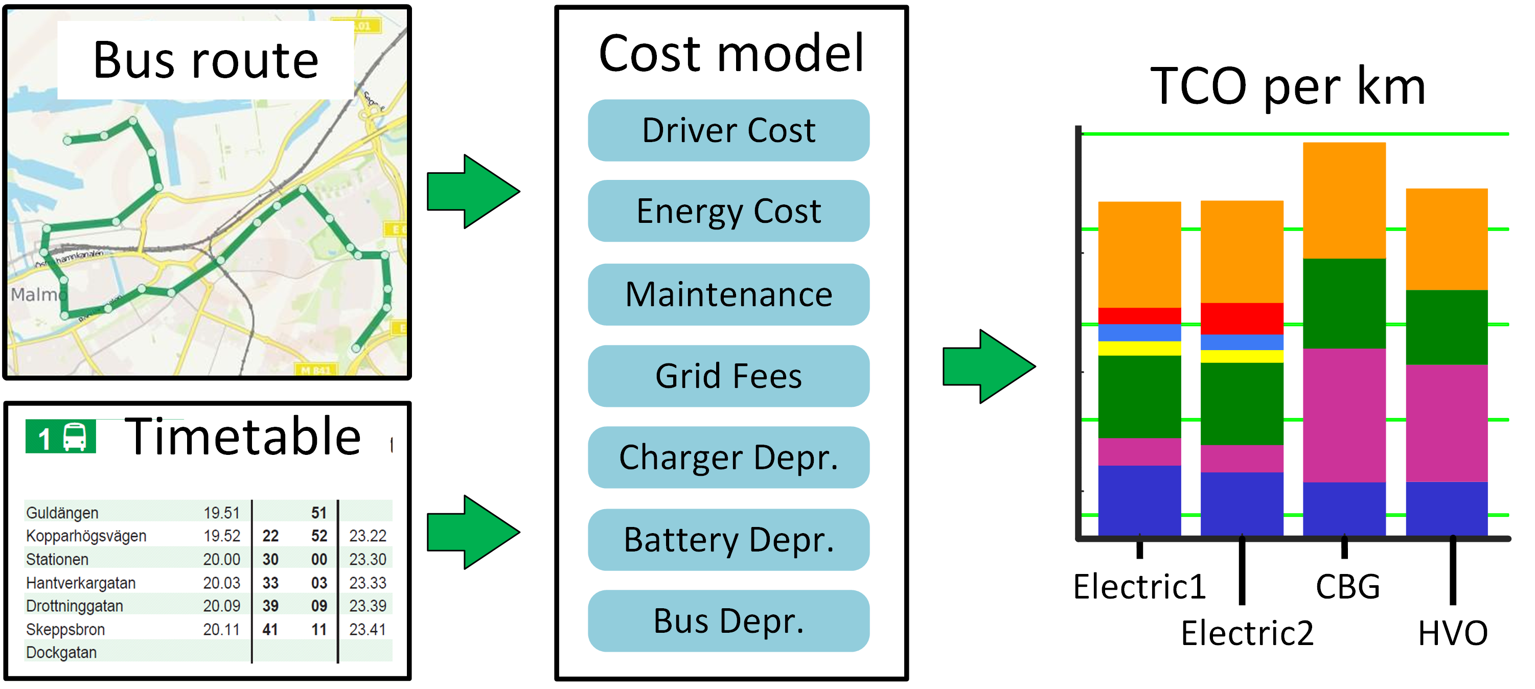
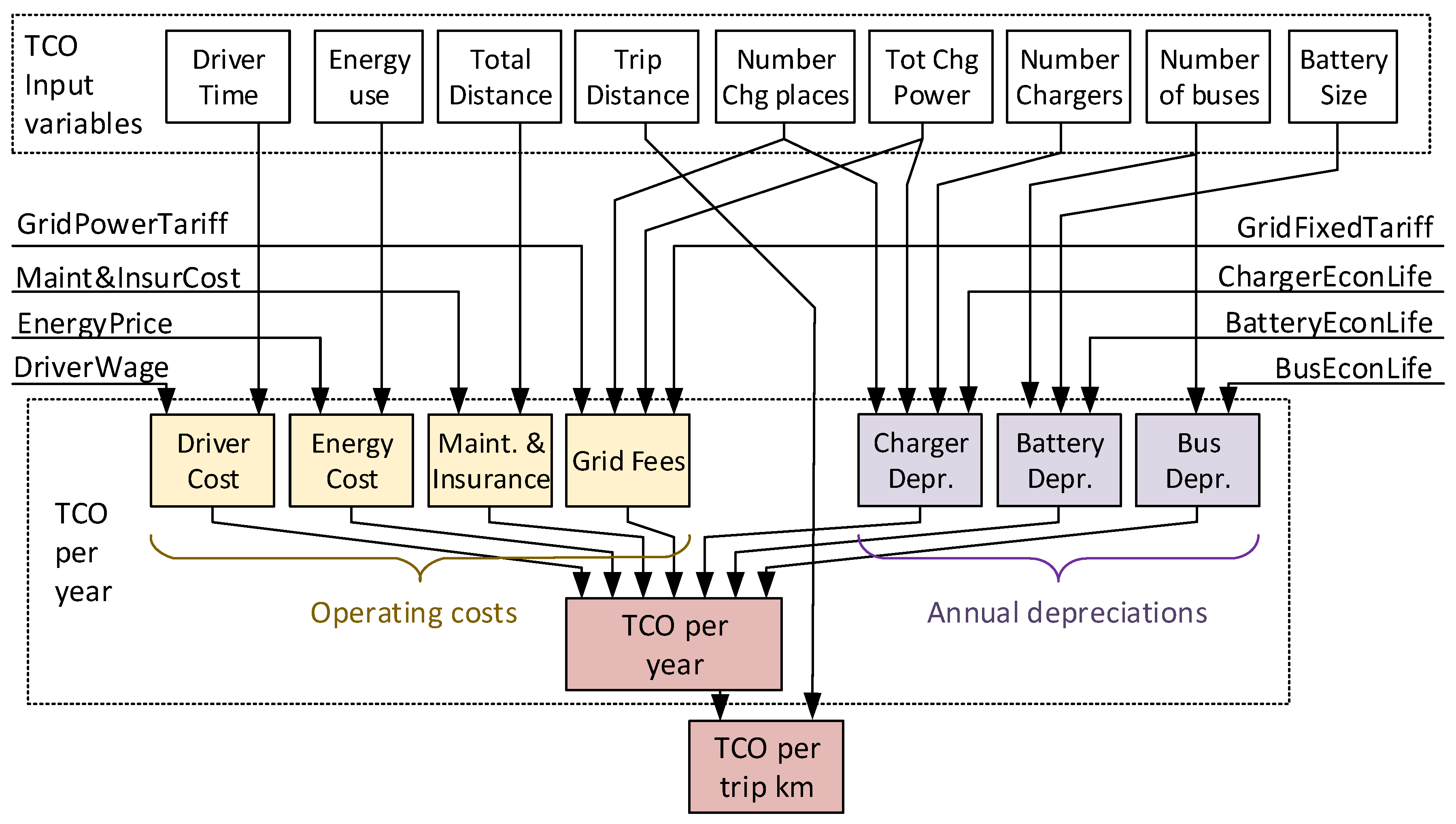
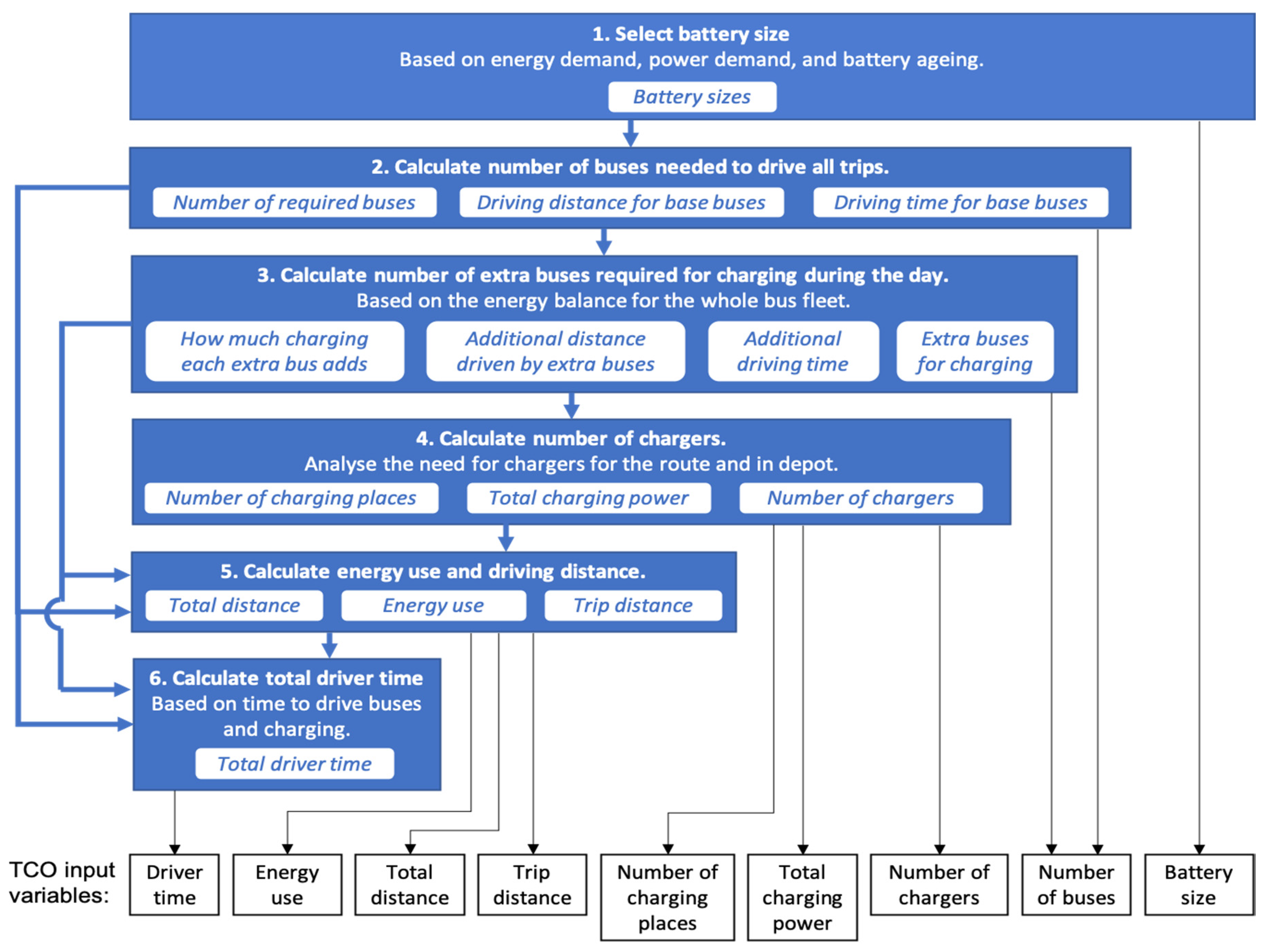
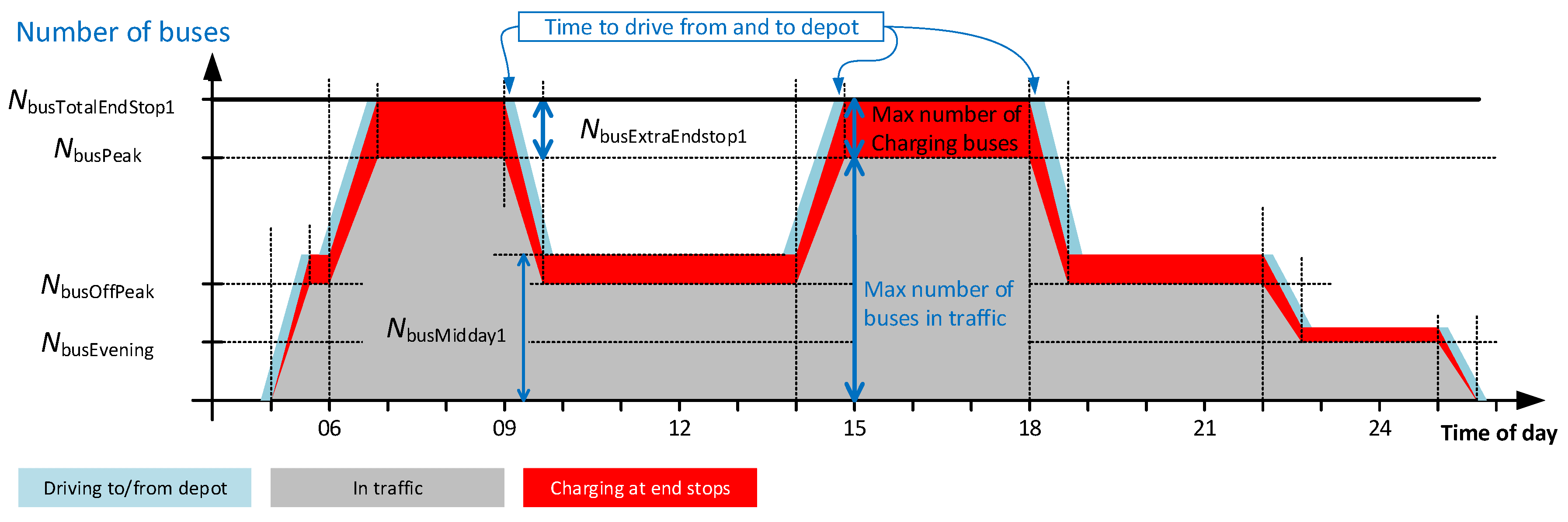
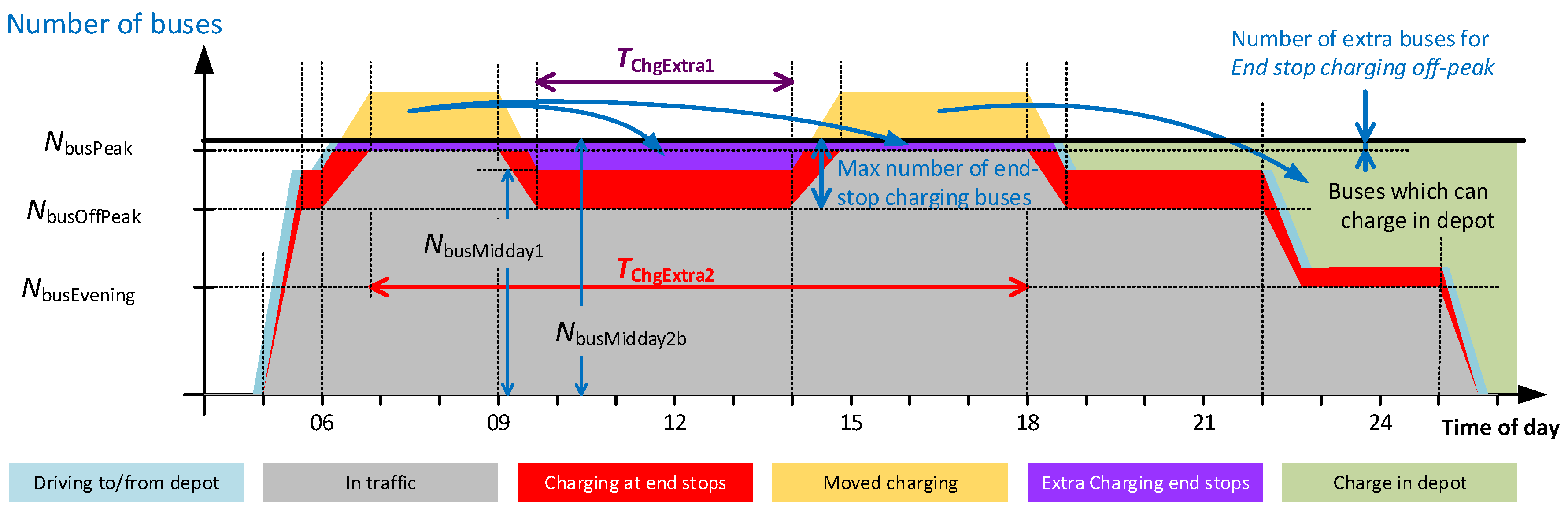
Table 1.
The cost parameters for buses powered by HVO, biomethane, and electricity when charging at the end stop, and at the end stop only during off-peak time. The values are relevant for Sweden 2019, and based on results from pilot projects.
Table 1.
The cost parameters for buses powered by HVO, biomethane, and electricity when charging at the end stop, and at the end stop only during off-peak time. The values are relevant for Sweden 2019, and based on results from pilot projects.
| Cost Parameters | HVO | Biomethane | Electricity | |
|---|---|---|---|---|
| End-Stop | End-Stop Off-Peak | |||
| Price (Million SEK) | 2.2 | 2.5 | 3 (excl. battery) | |
| Battery capacity (kWh) | - | - | 100 | 200 |
| Max energy used between charging (kWh) | - | - | 25 | 75 |
| Maintenance including chargers (SEK/km) | 3 | 3.6 | 3.3 | 3.3 |
| Bus Economic Life (year) | 10 | 10 | 10 | 10 |
| Battery Economic Life (year) | - | - | 7 | 7 |
| Battery Price (SEK/kWh) | - | - | 4000 | 4000 |
| Energy Cost (SEK/kWh) | 3.5 | 4 | 0.82 | 0.82 |
© 2020 by the authors. Licensee MDPI, Basel, Switzerland. This article is an open access article distributed under the terms and conditions of the Creative Commons Attribution (CC BY) license (http://creativecommons.org/licenses/by/4.0/).
Share and Cite
MDPI and ACS Style
Grauers, A.; Borén, S.; Enerbäck, O. Total Cost of Ownership Model and Significant Cost Parameters for the Design of Electric Bus Systems. Energies 2020, 13, 3262. https://0-doi-org.brum.beds.ac.uk/10.3390/en13123262
AMA Style
Grauers A, Borén S, Enerbäck O. Total Cost of Ownership Model and Significant Cost Parameters for the Design of Electric Bus Systems. Energies. 2020; 13(12):3262. https://0-doi-org.brum.beds.ac.uk/10.3390/en13123262
Chicago/Turabian StyleGrauers, Anders, Sven Borén, and Oscar Enerbäck. 2020. "Total Cost of Ownership Model and Significant Cost Parameters for the Design of Electric Bus Systems" Energies 13, no. 12: 3262. https://0-doi-org.brum.beds.ac.uk/10.3390/en13123262
Note that from the first issue of 2016, this journal uses article numbers instead of page numbers. See further details here.