Induction Motor Adaptive Backstepping Control and Efficiency Optimization Based on Load Observer

Abstract

In this paper, an adaptive load torque observer based on backstepping control is designed, which achieves accurate load estimation where the load is unknown. Based on this, in order to reduce the loss of the motor at low load, a smooth switching strategy of rotor flux based on speed error is designed. According to the real-time speed error of the induction motor, the smooth switching strategy achieves dynamic flux switching. Firstly, when the uncertain load occurs for the first time in the recursive design, the adaptive law of the load is designed, and a novel adaptive load torque observer is obtained, which accurately estimates the uncertain load torque in real time. Secondly, the relationship between the loss and the rotor flux is established by analyzing the loss model of induction motor, and the optimal rotor flux is obtained. The smooth switching control strategy based on speed error is designed to realize the efficiency optimization of induction motor. Finally, the control strategy proposed in this paper is experimentally verified on the LINKS-RT platform. The results show that the proposed control strategy has excellent load disturbance attenuation performance and reduces the energy loss.

1. Introduction

Induction motors (IMs) are widely used in electric vehicles and industrial robots due to reliability, high power density and excellent speed regulation performance [1,2,3]. The conventional proportional-integral (PI) control strategy has been applied in induction motor (IM) speed control system, which is easy to implement [4]. However, it is usually operated under rated flux, the loss of motor is large, and it has a weak performance in load disturbance attenuation. In modern industrial applications, the variable frequency speed control system of IM requires not only requires excellent control performance, but also requires the reduction of motor energy loss.

Actually, the control performance of IM drive system is easily affected by compounded disturbances, including parameters variation and external load disturbance [5,6,7]. In addition, external load disturbance can inevitably influence the control performance, bringing out speed fluctuation. Advanced control schemes have been utilized in speed control of IM drives for obtaining perfect load disturbance attenuation and speed response, such as sliding mode control [8,9], active disturbance rejection control [10,11], neural network control [12,13], fuzzy control [14,15], port-controlled Hamiltonian control [16,17,18] and so on. The Elman neural network control algorithm is designed in rotor position of IM drives application, which approximates the parameter uncertainties and lumped disturbances [12]. In Reference [14], a self-tuning algorithm is proposed to automatically adjust the output factor of the fuzzy logic speed controller, which improves the control effect of the fixed parameter fuzzy logic control algorithm in parameter variations and load disturbance. Nevertheless, the selection of fuzzy rules depends on human experience, which brings difficulty to the realization of the algorithm. The sliding mode algorithm is a complex control strategy which improves the ability of robustness to variable motor parameters and load disturbance attenuation. It has an attractive application prospect for the design of controllers and observers of motor drive system, realizing accurate estimation of load disturbance as well as obtaining satisfactory control performance [19,20]. In Reference [19], the second-order sliding mode disturbance observer is used to observe the disturbances, including motor parameters change and unmodeled dynamics. The output of the designed sliding mode disturbance observer is utilized as feedforward compensation to correct the current error caused by traditional deadbeat predictive current controller. In Reference [20], the second-order sliding mode control strategy is applied to the IM servo system to overcome the shortcomings of the first-order sliding mode control. The higher sampling frequency is applied in order to improve the dynamic performance in drive system, but with the increase of the sampling frequency, the hardware requirements are higher, which brings difficulty to the later experimental verification.

The backstepping control algorithm constructs the control law of IM by selecting Lyapunov function, which is applied to ensure the system stability and is widely used in the servo drive system [21,22,23]. In Reference [23], the improved backstepping nonlinear technology is equipped with an observer, which shows the superiority in robustness and speed response. The design idea of backstepping control technology is to recursively select the appropriate state variables as the virtual control input of low dimensional subsystem. Each backstepping design step generates a new virtual control variable, which is represented by the previous design step, and the final Lyapunov function is the sum of the Lyapunov functions designed in the previous recursive steps [24]. The backstepping control strategy is combined with the adaptive scheme, which has a superior property [25,26]. In Reference [26], the backstepping control strategy is combined with the adaptive mechanism to identify the rotor resistance of the induction motor on line. The designed rotor resistance observer has good performance in load disturbance and speed change, which improves the robustness of the control system.

IMs have significant efficiency optimization control effects when they are at light load operations [27,28]. In the traditional field oriented control technique, the rotor flux is constant in order to realize high dynamic performance, but it is detrimental for efficiency optimization [29]. Among the existing loss minimization control strategies, the loss model control has a faster convergence speed than the search control and is easy to implement, which has caused extensive research [30,31]. The loss model control establishes the relationship between the total loss and the rotor flux through the equivalent circuit in the stationary reference frame of the IM, and obtains the optimal rotor flux when the loss is minimal. In order to improve the system dynamic performance degradation caused by the optimal rotor flux in the efficiency optimization control, the rotor flux of the drive system is restored to the given rotor flux when the speed or load changes suddenly [32]. In Reference [28], low pass filter, torque producing current compensation to speed controller and variable structure speed controller in model based control of IM drives are discussed. Three control strategies are proposed to improve the dynamic performance of the system, and to save energy during sudden load transitions. However, when the motor changes from the optimal rotor flux to the given rotor flux in case of sudden speed and load torque, it is switched according to the time point of sudden change. In many practical applications, it is difficult to determine the time point when the running state of the motor changes (speed or load mutation).

In this paper, a novel adaptive load torque observer based on speed error and load torque error is proposed inspired from the work investigated in Reference [33]. The load torque adaptive law is presented in the first recursive design step, and a novel adaptive load torque observer is obtained compared with the conventional adaptive backstepping control strategy [34]. The designed observer accurately estimates the unknown load online, and achieves excellent speed control of IM. The Gaussian smooth switching control method based on the speed error realizes dynamic flux switching, which improves the efficiency of the motor at low load operation. The LINKS-RT experimental platform verifies the effectiveness of the proposed control algorithm in unknown load torque estimation, speed tracking performance, and smooth switching of rotor flux.

The organization of this paper is described below—Section 2 is devoted to the mathematical model of IM. Section 3 provides the design of control strategy including rotor flux observer, novel adaptive backstepping control. Section 4 is devoted to the optimization of efficiency through smooth switching control of the rotor flux. The experimental results are discussed in Section 5. Section 6 describes the conclusions.

2. Mathematical Model of IM

The mathematical model of IM on the $d-q$ axis can be presented by the following equation under the field oriented control strategy [26].

$$\begin{array}{c}\left\{\begin{array}{c}{\dot{i}}_{sd}=\upsilon i_{sd}+(n_p\omega +\frac{L_m{R}_r{i}_{sq}}{L_r{\lambda }_{rd}})i_{sq}+\frac{L_m{R}_r}{\sigma L_s{L}_r^2}{\lambda }_{rd}+\frac{1}{\sigma L_s}{u}_{sd}\hfill \\ {\dot{i}}_{sq}=\upsilon i_{sq}-(n_p\omega +\frac{L_m{R}_r{i}_{sq}}{L_r{\lambda }_{rd}})i_{sd}-\frac{L_m{n}_p\omega }{\sigma L_s{L}_r}{\lambda }_{rd}+\frac{1}{\sigma L_s}{u}_{sq}\hfill \\ {\dot{\lambda }}_{rd}=\frac{L_m{R}_r}{L_r}{i}_{sd}-\frac{R_r}{L_r}{\lambda }_{rd}\hfill \\ \dot{\omega }=\frac{1}{J}(T_e-T_L-B\omega ),\hfill \end{array}\right.\end{array}$$

(1)

where $\sigma =1-L_m^2/\phantom{L_m^2\left(L_r{L}_s\right)}\left(L_r{L}_s\right)$ is leakage coefficient, $\upsilon =-(L_m^2{R}_r+L_r^2{R}_s)/\phantom{(L_m^2{R}_r+L_r^2{R}_s)(\sigma L_s{L}_r^2)}(\sigma L_s{L}_r^2)$, and $T_e=\left(3n_p{L}_m{\lambda }_{rd}{i}_{sq}\right)/\phantom{\left(3n_p{L}_m{\lambda }_{rd}{i}_{sq}\right)\left(2L_r\right)}\left(2L_r\right)$ is electromagnetic torque. $u_{sd}$, $u_{sq}$, $i_{sd}$ and $i_{sq}$ stand for the component of stator voltage and current on the $d-q$ axis. $L_m$, J, B, $n_p$ and $T_L$ present mutual inductance, moment of inertia, friction coefficient, pole pairs and load torque. $L_s$ and $L_r$ are stator inductance and rotor inductance. ${\lambda }_{rd}$ and $\omega$ are rotor flux and mechanical angular speed of rotor.

The angular speed of $d-q$ axis ${\omega }_e$, the slip angular frequency ${\omega }_s$ and the electrical angular speed ${\omega }_r$ of IM are presented as [23]

$${\omega }_e={\omega }_s+{\omega }_r=\frac{L_m{R}_r}{L_r{\lambda }_{rd}}{i}_{sq}+n_p\omega .$$

(2)

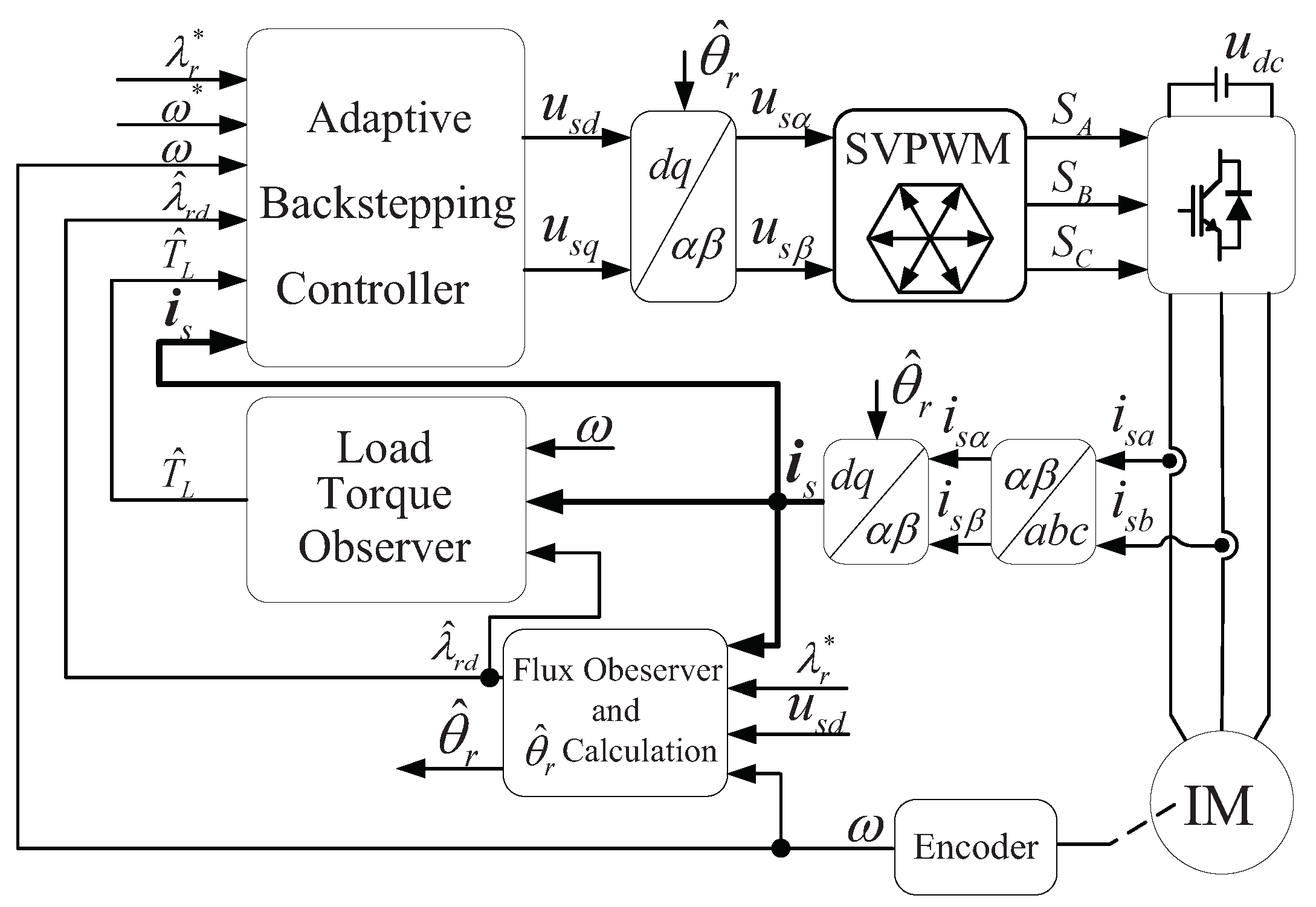
The block diagram of IM drive system based on the novel adaptive load torque observer is shown in Figure 1. ${\omega }^{*}$ and ${\lambda }_r^{*}$ are the given speed and rotor flux. ${\widehat{T}}_L$ and ${\widehat{\lambda }}_{rd}$ are the estimations of ${\widehat{T}}_L$ and ${\lambda }_{rd}$. ${\mathit{i}}_s$ is the stator current, and ${\mathit{i}}_s={\left[\begin{array}{cc}{i}_{sd}\hfill & i_{sq}\end{array}\right]}^T$. ${\widehat{\theta }}_r$ is the estimated value of the rotor flux position of the motor, which will be used for Clark transformation and Park transformation.

3. Design of Control Strategy

3.1. Rotor Flux Observer

It can be obtained from the rotor flux formula in Equation (1) that the rotor flux observer can be estimated from the stator current $i_{sd}$.

$${\dot{\widehat{\lambda }}}_{rd}=\frac{L_m{R}_r{i}_{sd}}{L_r}-\frac{R_r{\widehat{\lambda }}_{rd}}{L_r}.$$

(3)

Define the rotor flux error $e_{\lambda }={\lambda }_{rd}-{\widehat{\lambda }}_{rd}$, then ${\dot{e}}_{\lambda }=-\frac{R_r{e}_{\lambda }}{L_r}$. Choosing Lyapunov function $V_1=e_{\lambda }^2/\phantom{e_{\lambda }^{2}2}2$, and the derivative of it is expressed as

$${\dot{V}}_1=e_{\lambda }{\dot{e}}_{\lambda }=-\frac{R_r{e}_{\lambda }^2}{L_r}\le 0,$$

(4)

if and only if $e_{\lambda }=0$, ${\dot{V}}_1=0$. According to the Lyapunov stability theory and the LaSalle invariant theory, the rotor flux observer is asymptotically stable.

3.2. Novel Adaptive Backstepping Controller

In order to achieve the goal of remarkable performance speed control, the backstepping control scheme is adopted. Considering the uncertain load disturbance, the novel adaptive load torque observer is designed to accurately estimate the change of load torque in real time based on the principle of backstepping control. The novel load adaptive law is different from the convention, which is presented when the load torque first appears.

Define speed error, rotor flux error and their time derivative

$$\left\{\begin{array}{c}{e}_{\omega }={\omega }^{*}-\omega \hfill \\ e_{\lambda }={\lambda }_{rd}^{*}-{\widehat{\lambda }}_{rd}\hfill \end{array}\right.$$

(5)

$$\left\{\begin{array}{c}{\dot{e}}_{\omega }={\dot{\omega }}^{*}-\dot{\omega }\hfill \\ {\dot{e}}_{\lambda }={\dot{\lambda }}_{rd}^{*}-{\dot{\widehat{\lambda }}}_{rd}.\hfill \end{array}\right.$$

(6)

Consider the Lyapunov function

$$V_2=\frac{1}{2}(e_{\omega }^2+e_{\lambda }^2+a^{-1}{\tilde{T}}_L^2),labeleq7$$

(7)

where parameter $a>0$. ${\tilde{T}}_L=T_L-{\widehat{T}}_L$, ${\tilde{T}}_L$ and ${\widehat{T}}_L$ are the error value and estimated value of load torque. The time derivative of $V_2$ is

$${\dot{V}}_2=e_{\omega }{\dot{e}}_{\omega }+e_{\lambda }{\dot{e}}_{\lambda }+a^{-1}{\tilde{T}}_L{\dot{\tilde{T}}}_L=e_{\omega }({\dot{\omega }}^{*}-\dot{\omega })+e_{\lambda }({\dot{\lambda }}_{rd}^{*}-{\dot{\widehat{\lambda }}}_{rd})-a^{-1}{\tilde{T}}_L{\dot{\widehat{T}}}_L.$$

(8)

The q-axis current error $e_{iq}$ and the virtual control current $i_{sq}^{*}$ are derived as

$$\left\{\begin{array}{c}{e}_{iq}=i_{sq}^{*}-i_{sq}\hfill \\ i_{sq}^{*}=\frac{2J{L}_r}{3n_p{L}_m{\widehat{\lambda }}_{rd}}({\dot{\omega }}^{*}-\kappa ),\hfill \end{array}\right.$$

(9)

where $\kappa$ is a function, which is given in Equation (11).

Combining Equations (1), (8) and (9), the Equation (8) can be rewritten as

$$\begin{array}{cc}\hfill {\dot{V}}_2& =\frac{3n_p{L}_m{\widehat{\lambda }}_{rd}}{2J{L}_r}{e}_{\omega }{e}_{iq}+e_{\omega }(\kappa +\frac{{\widehat{T}}_L}{J}+\frac{B\omega }{J})+e_{\lambda }({\dot{\lambda }}_{rd}^{*}-\frac{L_m{R}_r}{L_r}{i}_{sd}+\frac{R_r}{L_r}{\widehat{\lambda }}_{rd})+{\tilde{T}}_L(\frac{e_{\omega }}{J}-a^{-1}{\dot{\widehat{T}}}_L)\hfill \\ \hfill & =\frac{3n_p{L}_m{\widehat{\lambda }}_{rd}}{2J{L}_r}{e}_{\omega }{e}_{iq}-k_1{e}_{\omega }^2-k_2{e}_{\lambda }^2-k_3{\tilde{T}}_L^2,\hfill \end{array}$$

(10)

where $k_i>0(i=1,2,3)$. Then the function $\kappa$, q-axis virtual control current $i_{sq}^{*}$ and load torque adaptive law are designed as

$$\left\{\begin{array}{c}\kappa =-k_1{e}_{\omega }-\frac{{\widehat{T}}_L}{J}-\frac{B\omega }{J}\hfill \\ i_{sd}^{*}=\frac{L_r}{L_m{R}_r}({\dot{\lambda }}_{rd}^{*}+\frac{R_r}{L_r}{\widehat{\lambda }}_{rd}+k_2{e}_{\lambda })\hfill \\ {\dot{\widehat{T}}}_L=a{k}_3{\tilde{T}}_L+a\frac{e_{\omega }}{J}.\hfill \end{array}\right.$$

(11)

By substituting (1) into (11), the load torque adaptive law is rewritten as

$${\dot{\widehat{T}}}_L=-a{k}_{3}J\dot{\omega }+\frac{a}{J}{e}_{\omega }+a{k}_3\left(\frac{3n_p{L}_m{\widehat{\lambda }}_{rd}}{2L_r}{i}_{sq}-{\widehat{T}}_L-B\omega \right).$$

(12)

According to Equation (12), the novel adaptive load torque observer can be expressed as

$${\widehat{T}}_L=-a{k}_{3}J{\int }_{\omega (0)}^{\omega (t)}d\omega +a{\int }_0^t\left[\frac{e_{\omega }}{J}+k_3\left(\frac{3n_p{L}_m{\widehat{\lambda }}_{rd}}{2L_r}{i}_{sq}-{\widehat{T}}_L-B\omega \right)\right]dt.$$

(13)

Substituting function $\kappa$ and (6) into (9), it can obviously get that

$${\dot{e}}_{\omega }=\frac{3n_p{L}_m{\widehat{\lambda }}_{rd}}{2J{L}_r}{e}_{iq}-k_1{e}_{\omega }+\frac{1}{J}{\tilde{T}}_L$$

(14)

$$i_{sq}^{*}=\frac{2J{L}_r}{3n_p{L}_m{\widehat{\lambda }}_{rd}}\left[k_1({\omega }^{*}-\omega )+\frac{1}{J}{\widehat{T}}_L+{\dot{\omega }}^{*}+\frac{B\omega }{J}\right].$$

(15)

Combining Equations (14) and (15), ${\dot{V}}_2$ can be described as

$${\dot{V}}_2=-k_1{e}_{\omega }^2-k_2{e}_{\lambda }^2-k_3{\tilde{T}}_L^2<0.$$

(16)

Choosing the Lyapunov function

$$V_3=V_2+\frac{e_{iq}^2}{2}.$$

(17)

Then, the time derivative of $V_3$ is given by

$$\begin{array}{cc}\hfill {\dot{V}}_3& =-k_1{e}_{\omega }^2-k_2{e}_{\lambda }^2-k_3{\tilde{T}}_L^2+\frac{2L_r}{3n_p{L}_m{\widehat{\lambda }}_{rd}}(k_1+a{k}_3-\frac{B}{J})e_{iq}{\tilde{T}}_L+e_{iq}(\frac{3n_p{L}_m{\widehat{\lambda }}_{rd}}{2J{L}_r}{e}_{\omega }\hfill \\ \hfill & +\frac{2J{L}_r}{3n_p{L}_m{\widehat{\lambda }}_{rd}}{k}_1{\dot{\omega }}^{*}-k_1{i}_{sq}+\frac{2k_1{L}_r}{3n_p{L}_m{\widehat{\lambda }}_{rd}}{\widehat{T}}_L+\frac{2L_r}{3n_p{L}_m{\widehat{\lambda }}_{rd}}B\omega +\frac{B}{J}{i}_{sq}\hfill \\ \hfill & +\frac{2L_r}{3J{n}_p{L}_m{\widehat{\lambda }}_{rd}}a{e}_{\omega }+\frac{2J{L}_r}{3n_p{L}_m{\widehat{\lambda }}_{rd}}{\ddot{\omega }}^{*}-\upsilon i_{sq}-\frac{2L_{r}B}{3n_{p}J{L}_m{\widehat{\lambda }}_{rd}}{\widehat{T}}_L-\frac{2L_r{B}^2}{3n_{p}J{L}_m{\widehat{\lambda }}_{rd}}\omega \hfill \\ \hfill & -\upsilon i_{sq}+{\omega }_e{i}_{sd}+\frac{L_m{\omega }_r}{\sigma L_s{L}_r}{\widehat{\lambda }}_{rd}-\frac{1}{\sigma L_s}{u}_{sq})\hfill \\ \hfill & =-k_1{e}_{\omega }^2-k_2{e}_{\lambda }^2-k_3{\tilde{T}}_L^2-k_4{e}_{iq}^2,\hfill \end{array}$$

(18)

where $k_4>0$. Equation (18) shows that the output $u_{sq}$ of controller is

$$\begin{array}{cc}\hfill u_{sq}=& \sigma L_s(k_4{e}_{iq}+\frac{3n_p{L}_m{\widehat{\lambda }}_{rd}}{2J{L}_r}{e}_{\omega }+\frac{2J{L}_r}{3n_p{L}_m{\widehat{\lambda }}_{rd}}{k}_1{\dot{\omega }}^{*}+\frac{2L_r}{3n_p{L}_m{\widehat{\lambda }}_{rd}}B\omega +\frac{B}{J}{i}_{sq}\hfill \\ \hfill & -k_1{i}_{sq}+\frac{2k_1{L}_r}{3n_p{L}_m{\widehat{\lambda }}_{rd}}{\widehat{T}}_L+\frac{2L_r}{3J{n}_p{L}_m{\widehat{\lambda }}_{rd}}a{e}_{\omega }-\frac{2L_{r}B}{3n_{p}J{L}_m{\widehat{\lambda }}_{rd}}{\widehat{T}}_L-\frac{2L_r{B}^2}{3n_{p}J{L}_m{\widehat{\lambda }}_{rd}}\omega \hfill \\ \hfill & +\frac{2J{L}_r}{3n_p{L}_m{\widehat{\lambda }}_{rd}}{\ddot{\omega }}^{*}-\upsilon i_{sq}+{\omega }_e{i}_{sd}+\frac{L_m{\omega }_r}{\sigma L_s{L}_r}{\widehat{\lambda }}_{rd}).\hfill \end{array}$$

(19)

Substituting (19) into (18) results in

$$\begin{array}{cc}\hfill {\dot{V}}_3=& -k_1{e}_{\omega }^2-k_2{e}_{\lambda }^2-k_4{e}_{iq}^2-{(\frac{\sqrt{k_3}}{\sqrt{2}}{\tilde{T}}_L-\frac{c}{\sqrt{2k_3}}{e}_{iq})}^2-{(\frac{\sqrt{k_3}}{\sqrt{2}}{\tilde{T}}_L-\frac{b}{\sqrt{2k_3}}{e}_{iq})}^2-(k_4-\frac{b^2+c^2}{2k_3})e_{iq}^2\hfill \end{array}$$

(20)

where $b=\frac{L_r}{n_p{L}_m{\widehat{\lambda }}_{rd}}{k}_1$, $c=\frac{L_r}{n_p{L}_m{\widehat{\lambda }}_{rd}}\left(a{k}_3-\frac{B}{J}\right)$.

Define current error of d-axis as $e_{id}=i_{sd}^{*}-i_{sd}$, choose the Lyapunov function as

$$V_4=\frac{e_{id}^2}{2}.$$

(21)

Obviously, ${\dot{V}}_4$ can be written as

$$\begin{array}{cc}\hfill {\dot{V}}_4& =e_{id}{\dot{e}}_{id}=e_{id}({\dot{i}}_{sd}^{*}-\upsilon i_{sd}-{\omega }_e{i}_{sq}-\frac{L_m{R}_r}{\sigma L_s{L}_r^2}{\widehat{\lambda }}_{rd}-\frac{1}{\sigma L_s}{u}_{sd})=-k_5{e}_{id}^2,\hfill \end{array}$$

(22)

where $k_5>0$. Then construct the control law $u_{sd}$

$$u_{sd}=\sigma L_s(k_5{e}_{id}+{\dot{i}}_{sd}^{*}-\upsilon i_{sd}-{\omega }_s{i}_{sq}-\frac{L_m{R}_r}{\sigma L_s{L}_r^2}{\widehat{\lambda }}_{rd}).$$

(23)

Substituting (23) into (22) results in

$${\dot{V}}_4=-k_5{e}_{id}^2<0.$$

(24)

4. Efficiency Optimized through Smooth Switching Control of Rotor Flux

The loss of IM includes stator iron loss, stator copper loss, rotor iron loss, and rotor copper loss. The rotor iron loss is ignored because it is small relative to the stator iron loss. The stator iron loss is represented by iron loss equivalent resistance $R_{\mathrm{Fe}}$, $i_{\mathrm{Fe}d}$ and $i_{\mathrm{Fe}q}$ are the currents through the resistance $R_{\mathrm{Fe}}$. The stable state equivalent circuit of IM can be shown in Figure 2 [27,35].

In the synchronous rotating coordinate system, the current of the $d-q$ axis is direct current, so the voltage of the two ends of mutual inductance $L_m$ in Figure 2 is zero. Based on the principle of rotor flux orientation, we have

$$\left\{\begin{array}{c}{i}_{\mathrm{Fe}d}=i_{sd}\hfill \\ i_{\mathrm{Fe}q}=i_{sq}+i_{rq}\hfill \end{array}\right.$$

(25)

$$\left\{\begin{array}{c}{\lambda }_{sd}={\lambda }_{rd}\hfill \\ {\lambda }_{sq}={\lambda }_{rq}=0,\hfill \end{array}\right.$$

(26)

where $i_{\mathrm{Fe}d}$ and $i_{\mathrm{Fe}q}$ are the d-q axis components of the current flowing through the equivalent resistance $R_{\mathrm{Fe}}$, ${\lambda }_{sd}$ and ${\lambda }_{sq}$ are stator flux of $d-q$ axis, ${\lambda }_{rd}$ and ${\lambda }_{rq}$ are rotor flux of $d-q$ axis. As shown in Figure 2, we have

$$i_{\mathrm{Fe}q}=\frac{{\omega }_e{\lambda }_{sd}}{R_{\mathrm{Fe}}}=\frac{{\omega }_e{\lambda }_{rd}}{R_{\mathrm{Fe}}}$$

(27)

$$i_{rq}=-\frac{{\omega }_s{\lambda }_{rd}}{R_r},$$

(28)

then

$${\omega }_s=-\frac{i_{rq}{R}_r}{{\lambda }_{rd}}=\frac{R_r}{{\lambda }_{rd}}(i_{sq}-i_{\mathrm{Fe}q})=(\frac{i_{sq}}{{\lambda }_{rd}}-\frac{{\omega }_r}{R_{\mathrm{Fe}}})\frac{R_r{R}_{\mathrm{Fe}}}{R_r+R_{\mathrm{Fe}}}.$$

(29)

The stator and rotor copper loss of IM can be expressed as

$$P_{\mathrm{Cu}s}=R_s(i_{sd}^2+i_{sq}^2)$$

(30)

$$P_{\mathrm{Cu}r}=R_r{i}_{rq}^2=\frac{R_r}{{(R_r+R_{\mathrm{Fe}})}^2}{(R_{\mathrm{Fe}}{i}_{sq}-{\omega }_r{\lambda }_{rd})}^2.$$

(31)

where $P_{\mathrm{Cu}s}$ and $P_{\mathrm{Cu}r}$ are stator and rotor copper loss. According to Equation (29), stator iron loss can be written as

$$P_{\mathrm{Fe}}=R_{\mathrm{Fe}}{i}_{\mathrm{Fe}q}^2=\frac{{\omega }_e^2}{R_{\mathrm{Fe}}}{\lambda }_{rd}^2=\frac{R_{\mathrm{Fe}}}{{(R_r+R_{\mathrm{Fe}})}^2}(R_r^2{i}_{sq}^2+2R_r{i}_{sq}{\omega }_r{\lambda }_{rd}+{\omega }_r^2{\lambda }_{rd}^2),$$

(32)

where $P_{\mathrm{Fe}}$ is stator iron loss. Combining Equations (30)–(32), the total loss $P_{loss}$ of IM is given by

$$P_{loss}=P_{\mathrm{Cu}s}+P_{\mathrm{Cu}r}+P_{\mathrm{Fe}}=(\frac{R_s}{L_m^2}+\frac{1}{R_r+R_{\mathrm{Fe}}}{\omega }_r^2){\lambda }_{rd}^2+(\frac{L_r^2}{n_p^2{L}_m^2}{R}_s+\frac{L_r^2{R}_r{R}_{\mathrm{Fe}}}{n_p^2{L}_m^2{R}_r+n_p^2{L}_m^2{R}_{\mathrm{Fe}}})\frac{T_e^2}{{\lambda }_{rd}^2}.$$

(33)

The efficiency of IM can be expressed as

$$\eta =\frac{{\omega }_r{T}_e}{{\omega }_r{T}_e+P_{loss}},$$

(34)

where $\eta$ is the operating efficiency of the motor.

Equation (33) shows that the loss of IM is a function of the rotor flux at a certain speed and electromagnetic torque. In order to reduce the loss in stable state, the purpose of efficiency optimization can be achieved by controlling the rotor flux. Let the first derivative of $P_{loss}$ to the rotor flux to be zero, we have

$${\lambda }_{ropt}^{*}=\sqrt[4]{\frac{L_r^2[R_r{R}_{\mathrm{Fe}}+R_s(R_r+R_{\mathrm{Fe}})]}{n_p^2[R_s(R_r+R_{\mathrm{Fe}})+{\omega }_r^2{L}_m^2]}}{\sqrt{T}}_e,$$

(35)

where ${\lambda }_{ropt}^{*}$ is the given value of the optimal rotor flux.

The Gaussian function based on speed error is used as the rotor flux coordination controller, which can dynamically switch the given flux. The smooth switching function is designed as

$$f(e_{\omega })=1-{\mathrm{e}}^{-{(e_{\omega }/S_d)}^2},$$

(36)

where $S_d$ is positive parameter. Adjust the $S_d$ to control the speed of smooth switching. Figure 3 shows the block diagram of the rotor flux smooth switching strategy. The output of rotor flux smoothing switching controller is designed as

$${\lambda }_{rnew}^{*}=f(e_{\omega }){\lambda }_r^{*}+[1-f(e_{\omega })]{\lambda }_{ropt}^{*},$$

(37)

where ${\lambda }_{rnew}^{*}$ is the value of the given flux calculated by the coordinated controller.

5. Experimental Results

In order to verify the effectiveness of the proposed control strategy in this paper, the experiment is carried out on the experimental setup developed by Beijing Links Corporation. The experimental setup is displayed in Figure 4. The experimental setup mainly consists of two servo drives (R&D servo drive and universal servo drive), two 1.5 KW squirrel cage IMs (drive motor and load motor), LINKS-RT real-time simulator and PC. The overall structure of the experiment is shown in Figure 5. The parameters of IM are shown in

Table 1. Parameters of IM.

Description	Value	Unit
Rated power	1.5	kW
Rated torque	9.6	Nm
Rated speed	1500	rpm
Stator resistance	0.96	$\mathsf{\Omega }$
Rotor resistance	0.93	$\mathsf{\Omega }$
Iron loss resistance	0.9	$\mathsf{\Omega }$
Stator inductance	0.11832	H
Rotor inductance	0.11867	H
Mutual inductance	0.11223	H
Moment of inertia	0.0038	$\mathrm{kg}·{\mathrm{m}}^2$
Friction coefficient	0.001	-
Pole pairs	2	-

. The switching frequency of the inverter is 10 kHz, and the sampling time of the control system is 0.0002 s. The parameters of novel adaptive load torque observer based on backstepping control are $k_1=150$, $k_2=100$, $k_3=3500$, $k_4=1150$, $k_5=2500$, $a=0.001$.

Case 1: At reference speed of 200 rpm, 600 rpm, 1000 rpm, and 1500 rpm, the robustness of the proposed control strategy under unknown load disturbances is tested, and the initial load torque is 1 Nm. 1 Nm load disturbance is added at t = 5 s and the load torque recovers to 1 Nm at t = 10 s. The given rotor flux is 0.2 Wb.

The detailed experimental curves are shown in Figure 6, Figure 7, Figure 8 and Figure 9. Figure 6a, Figure 7a, Figure 8a and Figure 9a show that the proposed algorithm can quickly converge to a given speed, and when the load suddenly increases (t = 5 s) and decreases (t = 10 s), the motor speed returns to the given speed after a short period of adjustment. Compared with the PI control method, the backstepping control method with the novel adaptive load torque observer (AB + LOB) has a shorter setting time and less overshoot. As shown in Figure 6b, Figure 7b, Figure 8b and Figure 9b the rotor flux observer can rapidly track the given rotor flux value under different speeds. Figure 6c, Figure 7c, Figure 8c and Figure 9c show the response curves of electromagnetic torque and load estimation. It can be seen that the proposed load observer can accurately estimate the value of uncertain load in real time. The A-phase current curves at different speeds are presented in Figure 6d, Figure 7d, Figure 8d and Figure 9d. From these figures, it can be seen that the amplitude of the A-phase current increases with the increase of the load torque.

Table 2. The detailed data comparison of Case 1.

Speed	Method	Setting Time	Load up S.F./A.T.	Load down S.F./A.T.
200 rpm	AB + LOB PI	0.18 s 0.22 s	53 rpm/0.28 s 71 rpm/0.31 s	40 rpm/0.31 s 42 rpm/0.33 s
600 rpm	AB + LOB PI	0.16 s 0.19 s	65 rpm/0.28 s 83 rpm/0.30 s	47 rpm/0.31 s 50 rpm/0.32 s
1000 rpm	AB + LOB PI	0.24 s 0.26 s	71 rpm/0.25 s 110 rpm/0.28 s	53 rpm/0.31 s 61 rpm/0.32 s
1500 rpm	AB + LOB PI	0.31 s 0.37 s	81 rpm/0.27 s 82 rpm/0.79 s	66 rpm/0.31 s 68 rpm/0.75 s

shows the detailed data comparison of Case 1. S.F. and A.T. represent speed fluctuation and adjustment time, respectively. From the experimental results of Case 1, the AB + LOB method realizes precise speed control, and has excellent load disturbance attenuation.

Case 2: The actual values of IM parameters (such as resistance, inductance and moment of inertia) are difficult to obtain. In order to analyze the robustness of the proposed control strategy under parameter changes, the following experiments are completed at a given speed of ${\omega }^{*}=600$ rpm.

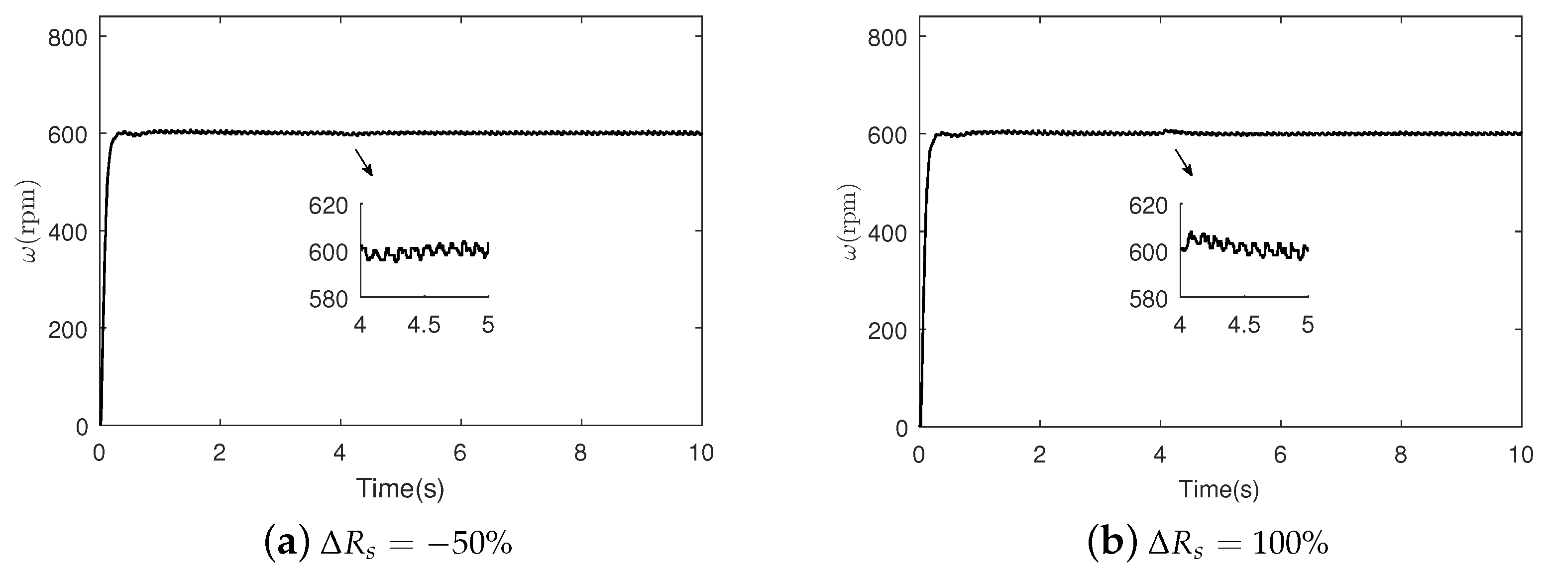
Considering that the actual parameters of IM cannot be changed arbitrarily, this paper verifies the robustness of the proposed algorithm to the parameters by changing the motor parameters used in the AB + LOB method. Suppose $X=X_n(1+\Delta X),X=(R_s,R_r,L_s,L_r,L_m,J)$, where X, $X_n$ and $\Delta X$ represent the actual value, nominal value and parameter variation degree of the motor parameters respectively. $\Delta X$ changes from $0\%$ to the given degree of variation at $t=4$ s. Figure 10, Figure 11, Figure 12 and Figure 13 show the experimental curves of parameters variation.

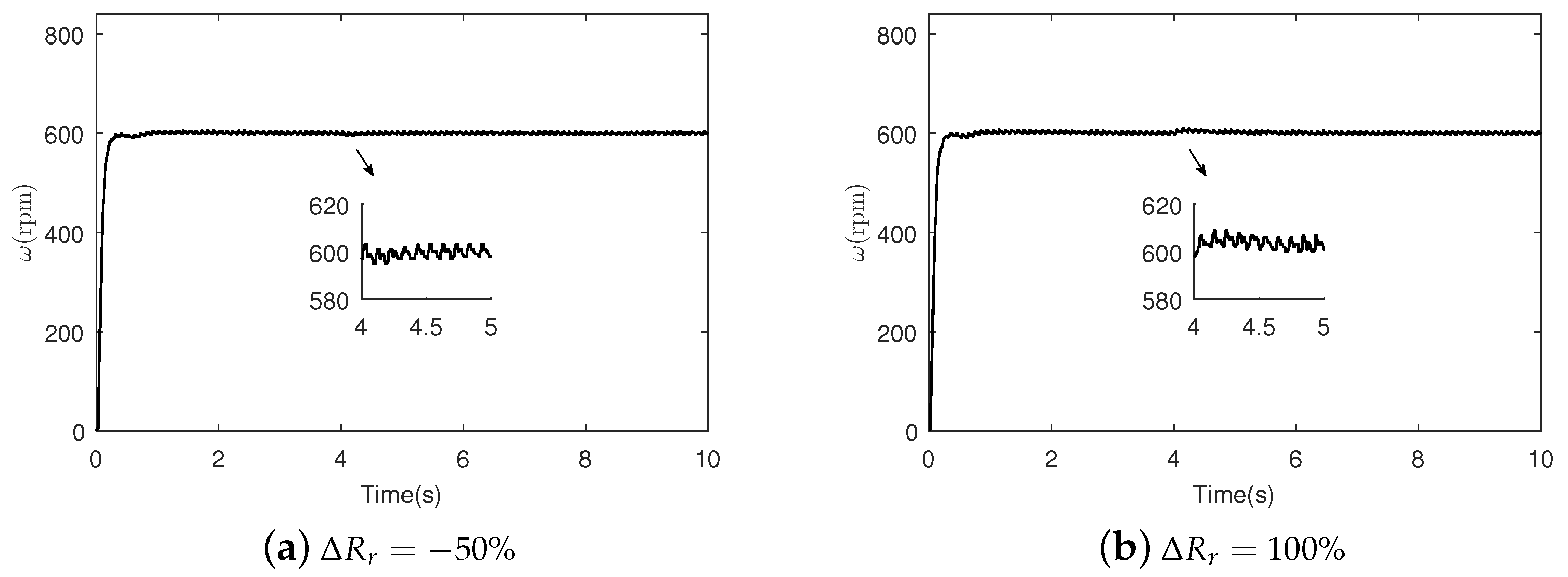
Figure 10 and Figure 11 show the speed curves of the motor under the proposed controller, in which the stator resistance value and the rotor resistance value change suddenly. Figure 10 shows that in the case where the stator resistance value is reduced by 50% and increased by 100%, the speed fluctuations are 1 rpm and 5 rpm, respectively. Figure 11 shows that in the case where the rotor resistance value is reduced by 50% and increased by 100%, the speed fluctuations are 1 rpm and 3 rpm, respectively.

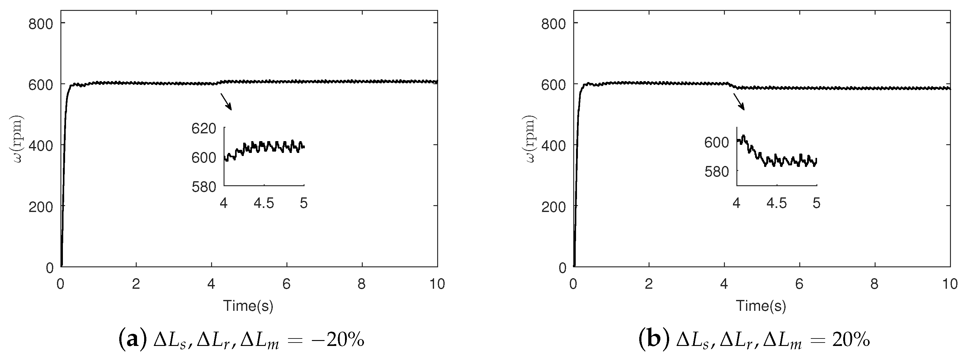
Figure 12 and Figure 13 show the proposed motor speed curve under the controller when the inductance value and the moment of inertia value change suddenly. Figure 12 shows that in the case where the inductance value is reduced by 20% and increased by 20%, the speed fluctuations are 5 rpm and 17 rpm, respectively. Figure 13 shows that when the moment of inertia value is reduced by 50% and increased by 50%, the speed fluctuations are 50 rpm and 20 rpm, respectively.

From the experimental results in Figure 11, Figure 12 and Figure 13, it can be concluded that the proposed speed controller has strong robustness for parameters variation.

Case 3: At reference speed of 600 rpm, the proposed smooth switching strategy for rotor flux based on a Gaussian function is verified. The load torque is 1 Nm at t = 0–10 s, and 1 Nm load disturbance is added at t = 10 s. The given rotor flux is 0.2 Wb. The positive parameter $S_d$ of the Gaussian function is chosen as 4.

As can be seen from Figure 14e, when the motor is at 600 rpm and the load torque is 1 Nm, the loss of the motor is 350 W. According to Equation (34), it can be calculated that $\eta \approx 77.4\%$. From Figure 14d,f, after applying the efficiency optimization control algorithm, the flux is 0.12 Wb and the loss of the motor is 180 W. According to Equation (34), it can be calculated that $\eta \approx 86.9\%$. When t = 10 s, the load torque increases to 2 Nm. From Figure 14b, the smooth switching algorithm still has a good speed response. From Figure 14e,f, it can be calculated that the efficiency of the motor before and after optimization is $86\%$ and $89.2\%$ respectively.

The experimental results in Case 3 verify the effectiveness of Gaussian function smooth switching control algorithm based on speed error. The proposed algorithm has a good speed response and reduces motor loss.

6. Conclusions

In this paper, a novel adaptive load torque observer and the smooth switching control strategy are proposed. The proposed load observer realizes accurate online estimation of unknown load disturbance. The proposed Gaussian smooth switching control method realizes the dynamic flux switching, and reduces the energy loss during the operation of the motor. The experimental results verify the effectiveness of the proposed method. With AB + LOB method, the motor speed control system has good dynamic and steady-state performance, and is robust to unknown load disturbance and parameters variation. With Gaussian smooth switching strategy, the running efficiency of the motor is improved under low load operation. However, the mismatch disturbances are not considered in this paper. Therefore, the future work will focus on eliminating the influence of mismatch disturbance on the motor system.

References

- Skowron, M.; Wolkiewicz, M.; Orlowska-Kowalska, T.; Kowalski, C.T. Application of Self-Organizing Neural Networks to Electrical Fault Classification in Induction Motors. Appl. Sci. 2019, 9, 616. [Google Scholar] [CrossRef] [Green Version]
- Carmenza, M.R.; Adolfo, A.J.M.; Juan, D.B.R. Stochastic Search Technique with Variable Deterministic Constraints for the Estimation of Induction Motor Parameters. Energies 2020, 13, 273. [Google Scholar]
- Nguyen, P.P.; Vansompel, H.; Bozalakov, D.; Stockman, K.; Crevecoeur, G. Inverse Thermal Identification of a Thermally Instrumented Induction Machine Using a Lumped-Parameter Thermal Model. Energies 2020, 13, 37. [Google Scholar] [CrossRef] [Green Version]
- Niu, L.; Xu, D.G.; Yang, M.; Gui, X.G.; Liu, Z.J. On-line Inertia Identification Algorithm for PI Parameters Optimization in Speed Loop. IEEE Trans. Power Electr. 2015, 30, 849–859. [Google Scholar] [CrossRef]
- Wang, B.; Luo, C.; Yu, Y.; Wang, G.L.; Xu, D.G. Antidisturbance Speed Control for Induction Machine Drives Using High-Order Fast Terminal Sliding-Mode Load Torque Observer. IEEE Trans. Power Electr. 2018, 33, 7927–7937. [Google Scholar] [CrossRef]
- Comanescu, M. Design and Implementation of a Highly Robust Sensorless Sliding Mode Observer for the Flux Magnitude of the Induction Motor. IEEE Trans. Energy Convers. 2016, 31, 649–657. [Google Scholar] [CrossRef]
- Li, J.; Ren, H.P.; Zhong, Y.R. Robust Speed Control of Induction Motor Drives Using First-Order Auto-Disturbance Rejection Controllers. IEEE Trans. Ind. Appl. 2015, 51, 712–720. [Google Scholar] [CrossRef]
- Ammar, A.; Bourek, A.; Benakcha, A. Nonlinear SVM-DTC for induction motor drive using input-output feedback linearization and high order sliding mode control. ISA Trans. 2017, 67, 428–442. [Google Scholar] [CrossRef]
- Liu, X.D.; Yu, H.S.; Yu, J.P.; Zhao, L. Combined Speed and Current Terminal Sliding Mode Control with Nonlinear Disturbance Observer for PMSM Drive. IEEE Access 2018, 6, 29594–29601. [Google Scholar] [CrossRef]
- Alonge, F.; Cirrincione, M.; D’Ippolito, F.; Pucci, M.; Sferlazza, A. Robust Active Disturbance Rejection Control of Induction Motor Systems Based on Additional Sliding-Mode Component. IEEE Trans. Ind. Electr. 2017, 64, 5608–5621. [Google Scholar] [CrossRef]
- Du, C.; Yin, Z.G.; Zhang, Y.P.; Liu, J.; Sun, X.D.; Zhong, Y.R. Research on Active Disturbance Rejection Control With Parameter Autotune Mechanism for Induction Motors Based on Adaptive Particle Swarm Optimization Algorithm With Dynamic Inertia Weight. IEEE Trans. Power Electr. 2019, 34, 2841–2855. [Google Scholar] [CrossRef]
- El-Sousy, F.F.M.; Abuhasel, K.A. Intelligent Adaptive Dynamic Surface Control System With Recurrent Wavelet Elman Neural Networks for DSP-Based Induction Motor Servo Drives. IEEE Trans. Ind. Appl. 2019, 55, 1998–2020. [Google Scholar] [CrossRef]
- Bouhoune, K.; Yazid, K.; Boucherit, M.S.; Chériti, A. Hybrid control of the three phase induction machine using artificial neural networks and fuzzy logic. Appl. Soft Comput. 2017, 55, 289–301. [Google Scholar] [CrossRef]
- Farah, N.; Talib, M.H.N.; Shah, N.S.M.; Abdullah, Q.; Ibrahim, Z.; Lazi, J.B.M.; Jidin, A. A Novel Self-Tuning Fuzzy Logic Controller Based Induction Motor Drive System: An Experimental Approach. IEEE Access 2019, 7, 68172–68184. [Google Scholar] [CrossRef]
- Saghafinia, A.; Ping, W.H.; Uddin, M.N.; Gaeid, K.S. Adaptive Fuzzy Sliding-Mode Control into Chattering-Free IM Drive. IEEE Trans. Ind. Appl. 2015, 51, 692–701. [Google Scholar] [CrossRef]
- Yu, H.S.; Yu, J.P.; Liu, J.; Song, Q. Nonlinear control of induction motors based on state error PCH and energy-shaping principle. Nonlinear Dyn. 2013, 72, 49–59. [Google Scholar] [CrossRef]
- Liu, X.D.; Yu, H.S.; Yu, J.P.; Zhao, Y. A Novel Speed Control Method Based on Port-Controlled Hamiltonian and Disturbance Observer for PMSM Drives. IEEE Access 2019, 7, 111115–111123. [Google Scholar] [CrossRef]
- Yu, H.S.; Yu, J.P.; Liu, J.; Wang, Y. Energy-shaping and L2 gain disturbance attenuation control of induction motor. Int. J. Innov. Comput. Inform. Control 2012, 8, 5011–5024. [Google Scholar]
- Wang, B.; Dong, Z.; Yu, Y.; Wang, G.L.; Xu, D.G. Static-Errorless Deadbeat Predictive Current Control Using Second-Order Sliding-Mode Disturbance Observer for Induction Machine Drives. IEEE Trans. Power Electr. 2018, 33, 2395–2403. [Google Scholar] [CrossRef]
- Teja, A.V.R.; Chakraborty, C.; Pal, B.C. Disturbance Rejection Analysis and FPGA-Based Implementation of a Second-Order Sliding Mode Controller Fed Induction Motor Drive. IEEE Trans. Energy Convers. 2018, 33, 1453–1462. [Google Scholar] [CrossRef]
- Fateh, M.; Abdellatif, R. Comparative study of integral and classical backstepping controllers in IFOC of induction motor fed by voltage source inverter. Int. J. Hydrogen Energy 2017, 42, 17953–17964. [Google Scholar] [CrossRef]
- Yu, J.P.; Ma, Y.M.; Yu, H.S.; Lin, C. Adaptive fuzzy dynamic surface control for induction motors with iron losses in electric vehicle drive systems via backstepping. Inform. Sci. 2017, 376, 172–189. [Google Scholar] [CrossRef]
- Zaafouri, A.; Regaya, C.B.; Azza, H.B.; Châari, A. DSP-based adaptive backstepping using the tracking errors for high-performance sensorless speed control of induction motor drive. ISA Trans. 2016, 60, 333–347. [Google Scholar] [CrossRef] [PubMed]
- Lin, F.J.; Wai, R.J.; Chou, W.D.; Hsu, S.P. Adaptive backstepping control using recurrent neural network for linear induction motor drive. IEEE Trans. Ind. Electr. 2002, 49, 134–146. [Google Scholar]
- Li, L.; Zhang, Z.C.; Wang, C.X. A flexible current tracking control of sensorless induction motors via adaptive observer. ISA Trans. 2019, 93, 180–188. [Google Scholar] [CrossRef]
- Regaya, C.B.; Farhani, F.; Zaafouri, A.; Chaari, A. A novel adaptive control method for induction motor based on Backstepping approach using dSpace DS 1104 control board. Mech. Syst. Signal Process. 2018, 100, 466–481. [Google Scholar] [CrossRef]
- Farhani, F.; Regaya, C.B.; Zaafouri, A.; Chaari, A. Real time PI-backstepping induction machine drive with efficiency optimization. ISA Trans. 2017, 70, 348–356. [Google Scholar] [CrossRef] [PubMed]
- Kumar, N.; Chelliah, T.R.; Srivastava, S.P. Adaptive control schemes for improving dynamic performance of efficiency-optimized induction motor drives. ISA Trans. 2015, 57, 301–310. [Google Scholar] [CrossRef] [PubMed]
- Kortas, I.; Sakly, A.; Mimouni, M.F. Optimal vector control to a double-star induction motor. Energy 2017, 131, 279–288. [Google Scholar] [CrossRef]
- Ammar, A.; Benakcha, A.; Bourek, A. Closed loop torque SVM-DTC based on robust super twisting speed controller for induction motor drive with efficiency optimization. Int. J. Hydrogen Energy 2017, 42, 17940–17952. [Google Scholar] [CrossRef]
- Abdelati, R.; Mimouni, M.F. Optimal control strategy of an induction motor for loss minimization using Pontryaguin principle. Eur. J. Control 2019, 49, 94–106. [Google Scholar] [CrossRef]
- Sousa, G.C.D.; Bose, B.K.; Cleland, J.G. Fuzzy logic based on-line efficiency optimization control of an indirect vector-controlled induction motor drive. IEEE Trans. Ind. Electr. 1995, 42, 192–198. [Google Scholar] [CrossRef]
- Butt, S.; Aschemann, H. Adaptive backstepping control for an engine cooling system with guaranteed parameter convergence under mismatched parameter uncertainties. Control Eng. Pract. 2017, 64, 195–204. [Google Scholar] [CrossRef]
- Tan, H. Field orientation and adaptive backstepping for induction motor control. In Proceedings of the 1999 IEEE Industry Applications Conference, Phoenix, AZ, USA, 3–7 October 1999; pp. 2357–2363. [Google Scholar]
- Cui, N.X.; Zhang, C.H.; Sun, F.T. Study on efficiency optimization and high response control of induction motor. Proc. CSEE 2005, 25, 118–123. [Google Scholar]
Figure 1.
Block diagram of induction motor (IM) drive system.
Figure 2.
Equivalent circuit of IM.
Figure 3.
Block diagram of rotor flux smooth switching strategy.
Figure 4.
Experimental setup.
Figure 5.
Overall structure of the experiment.
Figure 6.
Response curves at 200 rpm.
Figure 7.
Response curves at 600 rpm.
Figure 8.
Response curves at 1000 rpm.
Figure 9.
Response curves at 1500 rpm.
Figure 10.
Speed response curves when the stator resistance value changes suddenly.
Figure 11.
Speed response curves when the rotor resistance value changes suddenly.
Figure 12.
Speed response curves when the inductance value changes suddenly.
Figure 13.
Speed response curves when the moment of inertia value changes suddenly.
Figure 14.
The response curve before and after efficiency optimization at 600 rpm.