Using a Crop Model to Benchmark Miscanthus and Switchgrass

Abstract

Crop yields are important items in the economic performance and the environmental impacts of second-generation biofuels. Since they strongly depend on crop management and pedoclimatic conditions, it is important to compare candidate feedstocks to select the most appropriate crops in a given context. Agro-ecosystem models offer a prime route to benchmark crops, but have been little tested from this perspective thus far. Here, we tested whether an agro-ecosystem model (CERES-EGC) was specific enough to capture the differences between miscanthus and switchgrass in northern Europe. The model was compared to field observations obtained in seven long-term trials in France and the UK, involving different fertilizer input rates and harvesting dates. At the calibration site (Estrées-Mons), the mean deviations between simulated and observed crop biomass yields for miscanthus varied between −0.3 t DM ha⁻¹ and 4.2 t DM ha⁻¹. For switchgrass, simulated yields were within 1.0 t DM ha⁻¹ of the experimental data. Observed miscanthus yields were higher than switchgrass yields in most sites and for all treatments, with one exception. Overall, the model captured the differences between both crops adequately, with a mean deviation of 0.46 t DM ha⁻¹, and could be used to guide feedstock selections over larger biomass supply areas.

1. Introduction

The much-needed transition to sustainable and decarbonized energy systems requires continual improvements in the performance of renewable alternatives to our current energy sources. In the transportation sector, biofuels have been emphasized in the past decades given their compatibility with current motoring technologies [1]. First-generation biofuels are currently faced with two fundamental challenges that constrain their development. First, concerns were raised regarding their impacts on food security and food prices [2]. Secondly, they may contribute to deforestation and other land-use changes, resulting in mixed savings in terms of greenhouse gas (GHG) emissions compared to their fossil-based counterparts. This led the European Parliament to cap their contribution at 7% of the final transport fuel consumption [3], despite setting more recently a target of 32% renewables in the EU’s gross final energy consumption by 2030, as well as a target of 14% renewable energy in the transport sector. In this ambitious policy package, attention has shifted to second generation (2G) biofuels that rely on generic, ligno-cellulosic feedstock, rather than the storage compartments of food crops.

One of the reasons for this shift lies in the fact that second-generation biofuels are more efficient in abating GHG emissions compared to fossil fuels, even when factoring in indirect land-use change effects [4]. This was confirmed by a recent meta-analysis involving 50 journal articles dealing with biofuel and bioelectricity pathways, concluding that these advanced biofuels stand the best chance of reducing GHG emissions by 50% or more compared to fossil fuels, whereas their first generation counterparts were unable to match this fraction [5]. However, the efficiency of 2G biofuels hinges on the performance of feedstock supply, in particular when relying on dedicated biomass crops. A wide variety of inedible herbaceous feedstocks can be used for this purpose [6]. Two of them, belonging to the Poaceae family, have been extensively studied in Europe and North America: miscanthus (Miscanthus × giganteus), a sterile hybrid crop originating in Asia, and switchgrass (Panicum virgatum), a widespread species from the United States. Both can be grown in a large range of latitudes, with life spans of about 20 years. Their high biomass yields (up to 20 t DM ha⁻¹ yr⁻¹) and large fractions of cellulose and hemicellulose make them attractive feedstocks for bio-based products [6,7].

Perennial crops in general also have low fertilizer input requirements [8,9], due to their strong rhizome development, dense root system and efficient nutrient recycling [10,11]. As a result, switchgrass and miscanthus are often characterized by lower GHG emissions per hectare than annual crops [12,13]. They may also provide additional benefits, including soil erosion mitigation, soil fertility improvements and increased biodiversity, by providing nesting, shelter and brood places for many invertebrates, including pollinators, wild mammals and birds, especially during winter [14,15]. Moreover, perennial grasses may be successfully grown on marginal or degraded lands, which would alleviate the competition with other potential uses over land [16].

Annual biomass yield potentials are paramount to the economics and environmental performance of crops, but remain subject to large variations over time and space and in relation to crop management practices. Process-based models have been developed to simulate these effects and some were adapted to perennial crops, including miscanthus and switchgrass. Examples include EPIC [17], DAYCENT [18], SWAT [19], STICS [20,21] and CERES-EGC [22]. These models were used to examine the effect of crop management on the yields of switchgrass and miscanthus, in particular their response to fertilizer nitrogen input rates or harvest dates. They may therefore provide guidance as to the selection of the most appropriate feedstock type and management practices for a given supply area [23], and optimize the overall value-chain design.

Alternatively, the performances of candidate energy crops may be compared on the basis of field experiments [24,25]. These provide reference points carrying less uncertainty than simulations from crop models, whose relative prediction errors may reach 20–30% [26]. However, these observations only pertain to a restricted set of locations. Meta-analyses encompassing a wider range of conditions can provide a more comprehensive picture, but only convey general trends. For instance, the study in [27] concluded that miscanthus yielded on average 56% more biomass than switchgrass, which would lead to a favoring of the former crop in general. However, under drier climate conditions switchgrass may prove more drought-tolerant, and outperform miscanthus [28].

Despite the importance of benchmarking candidate crops when designing biomass supply chains, agro-ecosystem models have rarely been used for this purpose. A study compared three perennial grasses in a region of the US with the DayCent model [29], but did not evaluate the capacity of this model to predict crop yields based on field observations. Thus, the question of whether agro-ecosystem models are able to capture differences between candidate feedstocks within a given pedo-climatic context remains open.

Here, we set out to test the capacity of an agro-ecosystem model CERES-EGC [22] in simulating the yields of miscanthus and switchgrass crops under similar pedoclimatic conditions, and in capturing their differences. The model was first adapted to miscanthus and switchgrass, and then calibrated using data from a long-term trial in France. It was subsequently tested against data from a network of experimental sites across France and the UK.

2. Material and Methods

2.1. Model Description

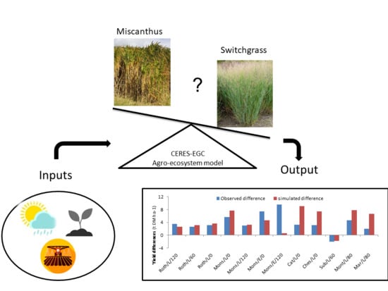
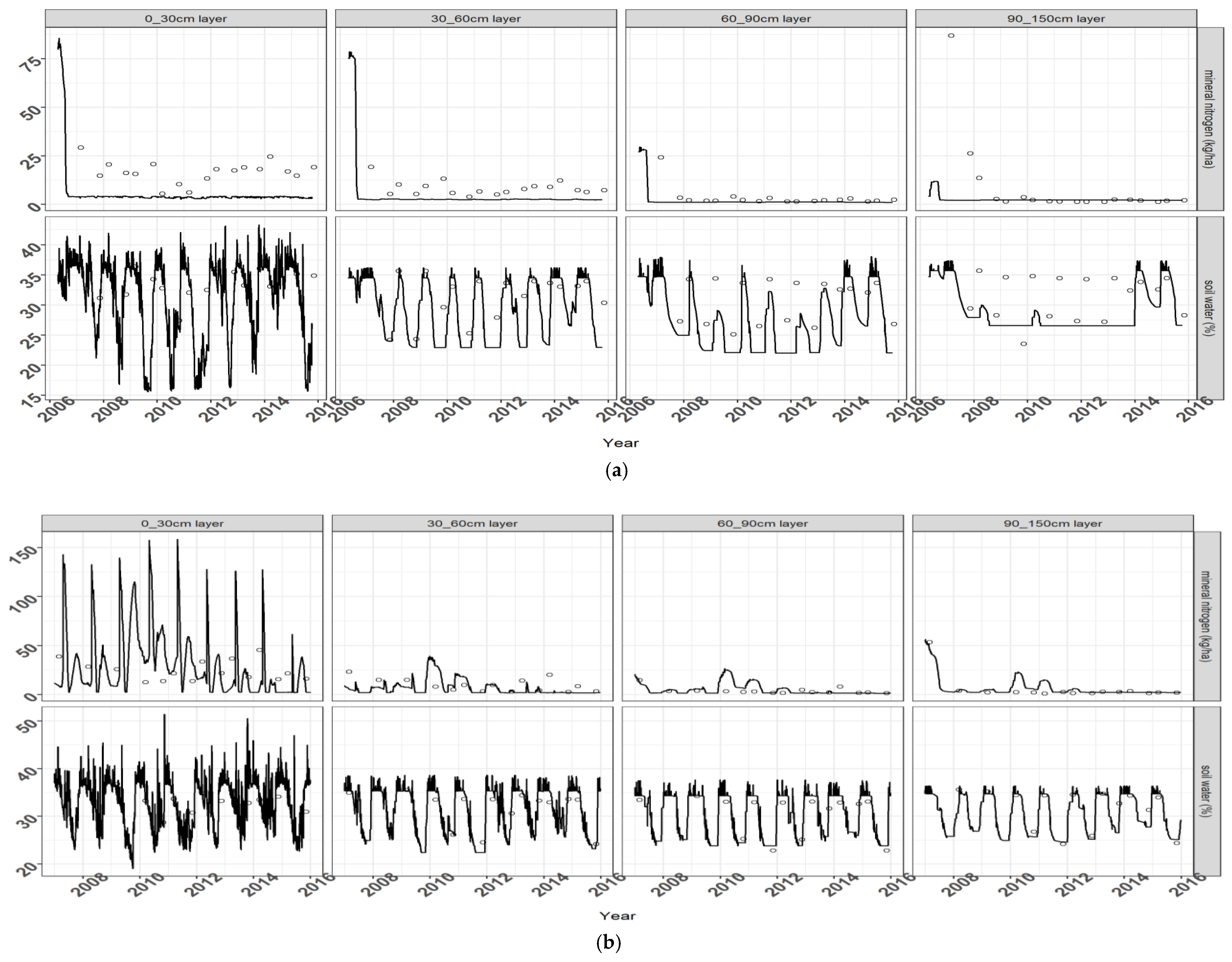
The following paragraphs describe the adaptation of CERES-EGC to the miscanthus and switchgrass crops. Most of the modeling concepts and equations apply to miscanthus, and the switchgrass version was evolved from the miscanthus routines by adjusting the relevant parameters, according to the literature on the ecophysiology of this particular crop.

2.1.1. General Characteristics

CERES-EGC evolved from the CERES suite of crop models [30], and is a process-based model describing soil–crop atmosphere processes in daily time steps with a focus on the simulation of environmental outputs such as N2O emissions [31]. It comprises sub-models accounting for different types of processes. A physical sub-model simulates the transfer of heat, water and nitrate down the soil profile, as well as soil evaporation, plant water uptake and transpiration in relation to climatic demand. A biological sub-model specific to each crop type simulates plant growth and phenological development. The latter drives the growth of various plant components (roots, leaves, stems) and the partitioning of photosynthates among them. A microbiological module simulates the turnover of organic matter in the plough layer, involving decomposition, mineralization and immobilization within three pools of organic matter, characterized by slow to fast turnover rates.

2.1.2. Model Inputs

The weather data needed to run CERES-EGC include daily values of solar radiation, maximum and minimum air temperature, precipitation and evapotranspiration. Soil input data include surface albedo, initial amount and C:N ratio of soil organic matter, soil water contents at wilting point, field capacity, saturation throughout the soil profile (which is divided into layers 10 to 30 cm in thickness), bulk density and stone content. Topsoil pH, clay and calcium carbonate contents are also required. The profiles of soil water and inorganic N contents have to be initialized at the beginning of the simulations, along with the various pools of soil organic C and N accounted for.

Crop management data include planting date and density, rates and types of fertilizer N inputs, dates and amounts of irrigation inputs, and harvest date.

2.1.3. Crop Development Stages

For miscanthus and switchgrass, five development stages were defined with a base temperature of 6 °C for miscanthus and 10 °C for switchgrass. The developmental stages of miscanthus are described below. They also apply to switchgrass.

Stage 1: Shoot emergence. This stage requires a minimum air temperature above 10 °C and daylengths longer than 12 hours.

Stage 2: Leaf growth. Leaves start growing after a thermal time of 900 GDD₆ (Growing Degree Day with a base temperature of 6 °C for miscanthus and 10 °C for switchgrass) has elapsed after emergence. The crop leaf area index (LAI) may increase up to a maximum value of 7.5.

Stage 3: Onset of leaf senescence. Crop LAI diminishes at a daily rate of 0.03 m² m⁻², which doubles when the plant enters its overall senescence (stage 4). This occurs after a thermal time of 3000 GDD₆ has elapsed. Photosynthesis continues during Stage 3, with all the photosynthates being allocated to rhizome. This stage may end prematurely if there are six consecutive days with an air temperature under 10 °C, a frost or 30 consecutive drought days [32]. At the end of this stage, leaves are assumed to have been entirely shed.

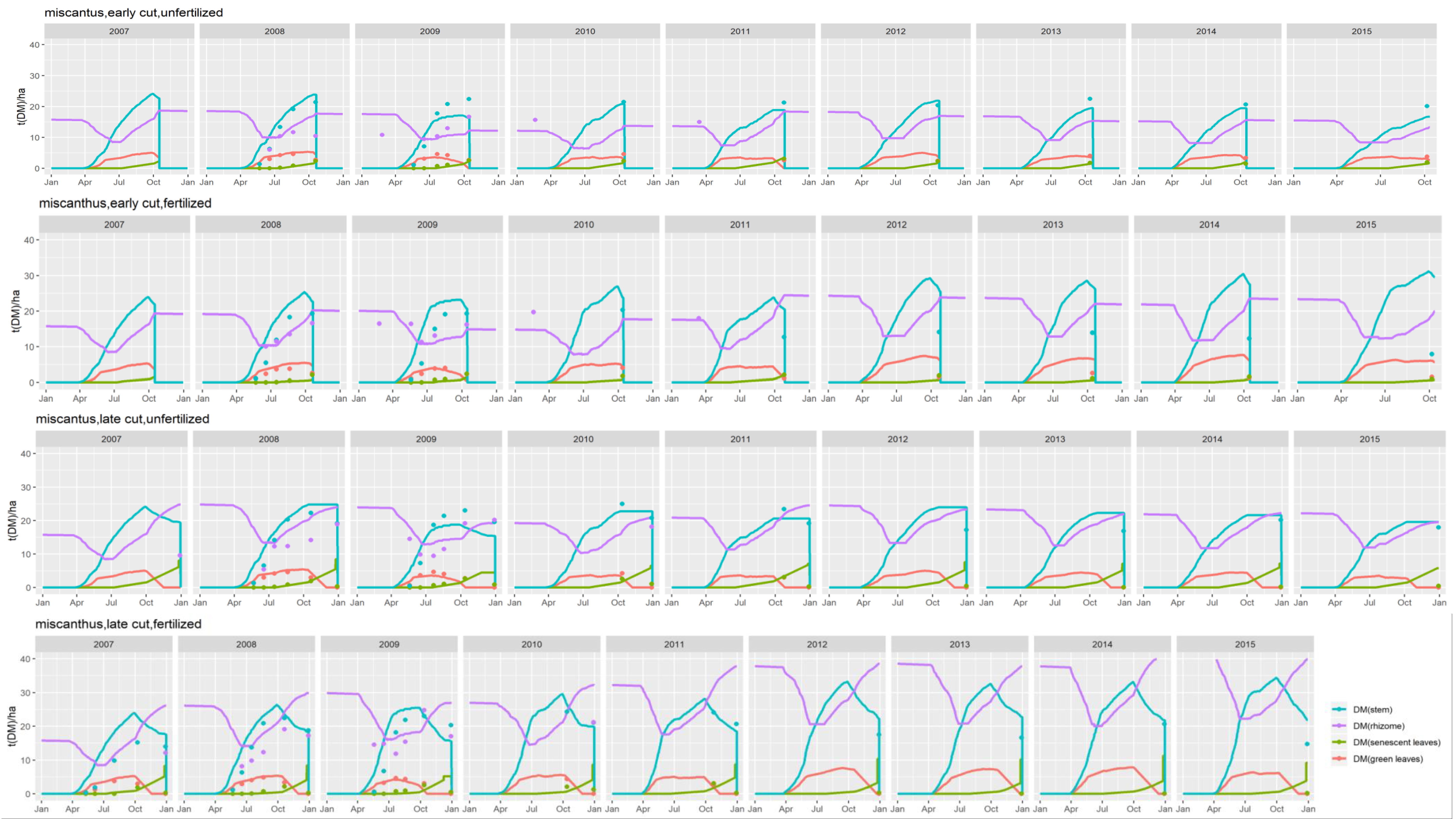
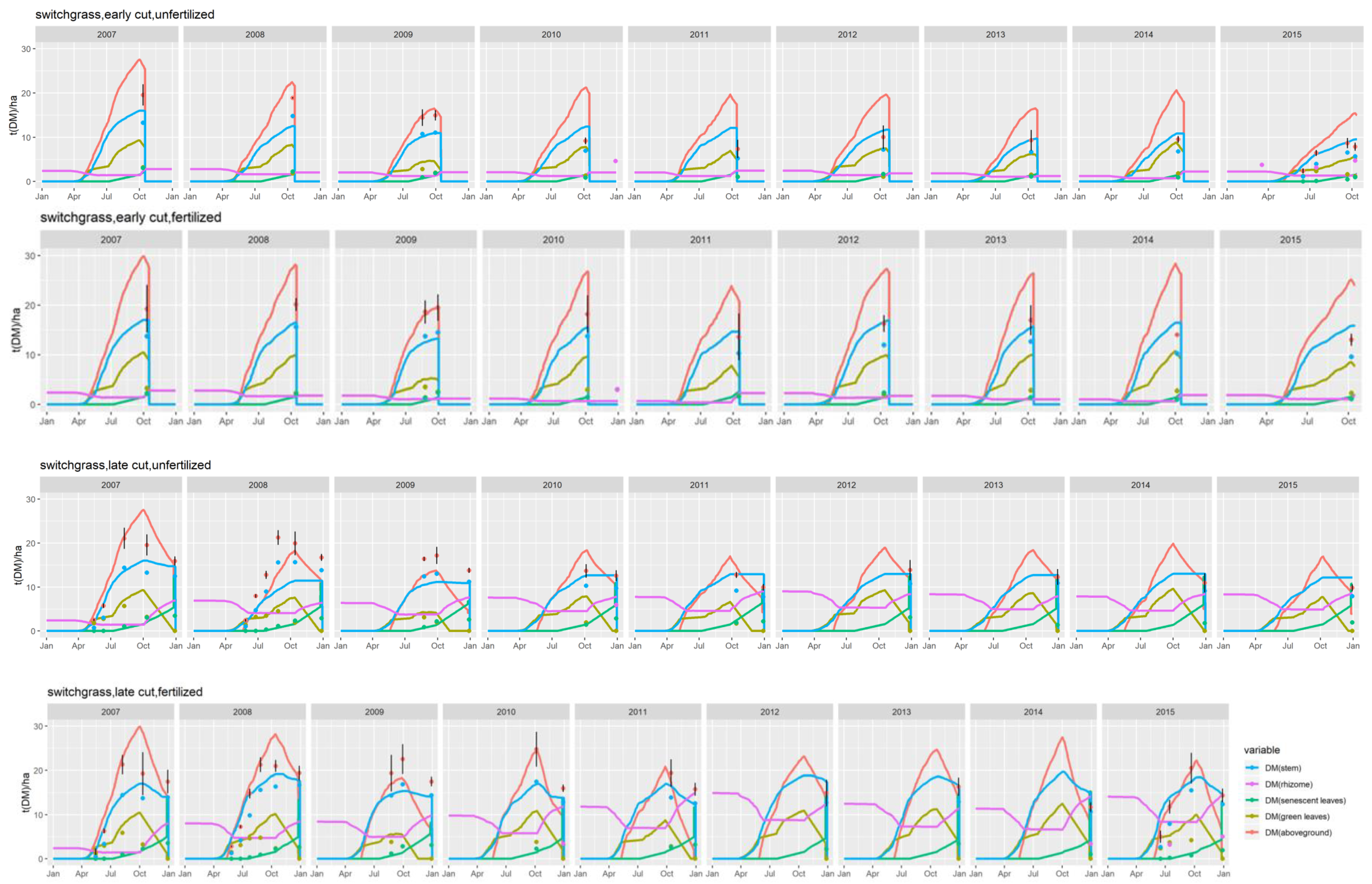
Stage 4: Onset of plant senescence. Photosynthesis stops and part of the stem biomass is translocated to the rhizomes. Stems dry up and are gradually shed until the day of harvest.

Stage 5: Dormancy. Plant growth stops until new shoots emerge.

2.1.4. Biomass Production, Partitioning, and Translocation

Plant growth and biomass partitioning. At the beginning of the simulation (stand establishment phase), miscanthus or switchgrass plants are only made up of their rhizomes and roots. Potential dry matter production is calculated through a radiation use efficiency (RUE) calculation. Potential dry matter production is based on light interception, as follows:

PCARB = PAR× (RUE(1 − exp(−k LAI)))

(1)

where PCARB is the potential aboveground dry matter production of the day (g DM m⁻²), PAR are the photosynthetically active radiations (MJ d⁻¹), and k the extinction coefficient.

The daily increase in plant dry matter (CARBO, g DM m⁻²) is calculated as:

CARBO = PCARB × min(NDEF, SWDF) + REMC

(2)

where SWDF and NDEF are 0–1 modifiers accounting for limitations through water and N stress (see corresponding section below), and REMC (g DM m⁻²) is a flux of biomass remobilized from rhizome to the aboveground parts of the plant. During the first two development stages, 45% of the miscanthus rhizome dry matter is transferred to aboveground [21]. A conversion efficiency of gross to net energy (or biomass) flow of 50% is assumed [21].

Daily plant growth is the sum of above- and below-ground biomass increments. Photosynthates are partitioned between the various plant compartments according to crop development stage, using partitioning variables for each stage and each compartment of the plant (

Table A1. Model parameter settings and calibrated values for miscanthus and switchgrass.

Term	Units	Definition	Miscanthus Value	Switchgrass Value	Origin of the Value
RUE	g·MJ−1	Radiation use efficiency	3.1	2.9	Calibrated
MATUR	Year	maturity age	5	5	Calibrated
DETRH	dimensionless ([0–1])	assimilates diverted to the rhizome during youth	0.3	0.5	Calibrated
PLFN	dimensionless ([0–1])	slope for N translocation from leaves	0.71	0.71	Calibrated
PSTMN	dimensionless ([0–1])	slope for N translocation from stems	0.51	0.51	adapted from [39]
BLFN	kgN·ha−1	intercept for N translocation from leaves	13	13	[39]
BSTMN	kgN·ha−1	intercept for N translocation from stems	13	13	Calibrated
STRSSW	dimensionless ([0–1])	adjustment for water stress	1.0	1.0	Calibrated
CRWU	cm3·water·cm−1 root	coefficient for root water uptake	0.1 × 10−3	6 × 10−3	Calibrated
ERWU	cm·cm−1	exponent for root water uptake	32	32	Calibrated
MASSUR	g·cm−2	leaf weight-to-area ratio	0.006	0.006	[40]
PLAGR	m2·m−2 (°Cd)−1	LAI growth rate per DTT	180	180	Fixed during calibration
DLAI	m2·leaf·m−2 soil·d−1	daily LAI decrease	0.03	0.03	[32]
SLA	g·DM·m−2	specific leaf area	60	60	Calibrated
RHNMX	gN·g−1	maximum rhizome nitrogen concentration	0.02	0.02	[39]
RH NMIN	gN·g−1	minimum rhizome nitrogen concentration	0.006	0.006	[39]
REP1ST	Dimensionless ([0–1])	dry matter partitioning to stems during stage 1	0.4	0.4	Adapted [40]
REP1RT	dimensionless ([0–1])	dry matter partitioning to roots during stage 1	0.1	0.1	Adapted [40]
RE P3ST	dimensionless ([0–1])	dry matter partitioning to stems during stage 3	0.4	0.2	Adapted [40]
RE PRTX X	dimensionless ([0–1])	maximum partitioning to roots during stage 3 and 4	0.5	0.9	Calibrated
RE PRTN	dimensionless ([0–1])	minimum partitioning to roots during stage 3 and 4	0.01	0.01	Calibrated
REPBG	dimensionless ([0–1])	total partitioning to below-ground biomass during stage 3 and 4	0.2	0.7	Calibrated
ST RUCN	gN·g−1	minimum aboveground N content	0.003	0.003	[39]
PARAMA	Dimensionless	allometric constant for N dilution curve	3	3	[39]
PARAMB	Dimensionless	exponent for N dilution curve	−0.47	−0.47	[39]
MAXN	gN·g−1	maximum N content at the beginning of growth	0.04	0.04	[39]
IDRANC	gN·g−1	root N content	0.006	0.006	Calibrated
RHW T IN	g·plant−1	rhizome weight at the beginning of shoot emergence	0.1	0.1	Calibrated
P2	°Cd	thermal duration to leaf growth	900	900	Adapted [32]
P3	°Cd	thermal duration to leaf senescence	2000	2000	Adapted [32]
P4	°Cd	thermal duration to plant senescence	3800	3800	Adapted [32]
K	m2·m−2	extinction coefficient	0.61	0.70	Calibrated
STRSSN	dimensionless ([0–1])	adjustment for nitrogen stress	0.8	1.0	Calibrated
P1	°Cd	not used	650	650	Calibrated
RE MN1	dimensionless ([0–1])	% rhizome nitrogen remobilized	0.79	0.79	[39]
RE MN2	kgN·ha−1	minimum nitrogen content	39	39	[39]
RINC	Dimensionless	root incorporation parameter	2	2	Calibrated
RINCF	Dimensionless	residue incorporation parameter	2	2	Calibrated
RWUMX	cm·cm−1	maximum root water uptake	0.03	0.03	Calibrated

). Before the stand reaches maturity, more photosynthates are allocated to below-ground compartments to ensure crop establishment. When maturity is reached (phenological Stage 2), all photosynthates are apportioned to aboveground biomass pools.

At the end of the first year, miscanthus or switchgrass stems are usually not harvested but cut and left on the soil surface. In the following years, the CERES-EGC model calculates biomass yields as the weight of plant stems and leaves, assuming 10% are left as stubbles and hence returned to the soil.

Leaf development. During leaf growth (phenological Stage 2), LAI expands at a relative rate of 0.018 m² m⁻² d⁻¹ for miscanthus [21], provided enough dry matter is available to maintain a constant specific leaf area (SLA). Leaf expansion is reduced accordingly if this is not the case. Leaf expansion is also modulated by leaf-specific nutrient and water stress modifiers (see corresponding section below). During leaf senescence LAI declines at a relative rate of 0.03 m² m⁻² d⁻¹ [21].

Roots. The root growth subroutine is adapted from the original CERES routine [30]. The initial root length density is set to 0.08 cm root cm⁻³ soil. The vertical elongation rate of roots is a function of thermal time, soil water and N contents. Root density may increase to a maximum value of 6 cm root cm⁻³ soil in the top 10 cm of soil, 3 cm root cm⁻³ soil in the 10–30 cm layer, and 1 cm root cm⁻³ soil below the 30 cm depth. Maximum rooting depth is set to 3 m.

Plant senescence. Root and rhizome senescence occur throughout the growing season with daily decay rates of 0.05% and 0.001%, respectively. Rhizome starts senescing only after a threshold mass value of 500 g DM m⁻² has been reached for this compartment. Senescent leaves that have dropped at the end of Stage 3, stems left on the ground after harvest, senescent roots and rhizomes are returned to the soil as fresh organic matter pools.

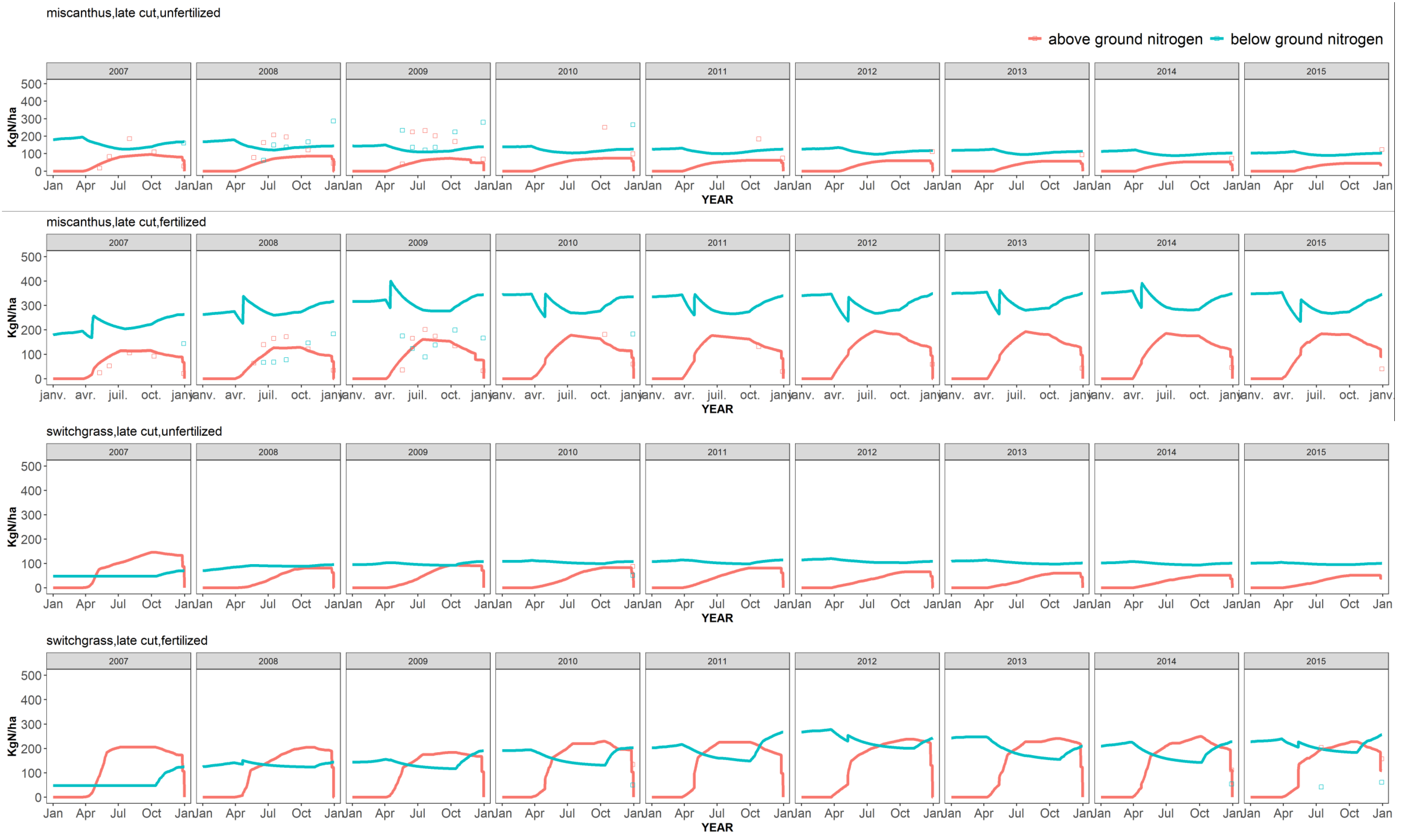
N and C fluxes within the plant. At the beginning of the growing season, a pool of rhizome N that can be potentially remobilized to the aerial parts (REMN, in g N m⁻²) is calculated as:

REMN = 0.56 × RHNIN – 39

(3)

where RHNIN is the rhizome nitrogen content in kg DM ha⁻¹.

Every day, rhizomes may contribute up to a maximum of REMN to the N demand, or until rhizome N has reached a minimum concentration of 0.6%, to prevent its total N depletion. Potential crop N uptake is a function of the amount of nitrate and ammonium available in each soil layer, and the corresponding root density [30]. From leaf senescence to harvest, if N uptake is larger than plant demand, excess N is stored in the rhizome up to a maximum concentration of about 2% [33].

During leaf and plant senescence, N is remobilized from the aboveground biomass to the rhizome. The daily N remobilization rates (denoted RHN, in g N m⁻² d⁻¹) depend on growing degree-days relative to the duration of the whole period of remobilization. They are calculated as [11]:

$$RHN=\frac{GD{D}_8}{P4-AP3}\times 0.71\times LFNIN-13$$

(4)

where LFNIN is the initial N contents of leaves (stems) at the beginning of leaf (stem) senescence, respectively (in g N m⁻²). P4-AP3 is the thermal time from the end of leaf senescence to plant senescence. N remobilization from the stems is supposed to occur between October and February. P8 is the thermal time from October to February. Stems and leaves keep a structural N concentration around 0.3% (on a mass basis [10]), and the remobilization is limited by a maximum rhizome N content of 2%.

Water and N stress. Similar to most crop models, the effect of N deficiencies on crop growth is calculated via a 0 to 1 modifier (stress factor) corresponding to a supply-to-demand ratio. Crop N demand is based on the concept of critical N concentration in plant biomass, i.e., the optimal concentration for biomass production depending on plant development stage. The definition of such concentrations for miscanthus is complicated by rhizome remobilization, and there are no data specific to this plant. We therefore used a generic allometric relationship for the aboveground biomass of annual and perennial crops:

N_crit% = aW^b

(5)

where N_crit% is the critical N concentration (%, mass basis), W is the aboveground biomass (g DM m⁻²), and a and b are parameters set at 3.0 and −0.47 for both crops. An upper limit of 4% was set for N_crit% for low W values, while root N concentration was set to 0.6%. [10].

Following the generic approach of the CERES models [30], the water stress effects on plant photosynthesis and development depend on the ratio of actual to potential plant transpiration, as modulated by an unitless parameter (WSTRSS) accounting for the particular sensitivity of miscanthus to water stress. Maximum plant transpiration is calculated from a Penman potential evapotranspiration rate (which is an input for the model), with a crop coefficient ranging between 0.8 and 1.1 depending on crop leaf area index. Root water uptake depends on soil available water and root density in each soil layer.

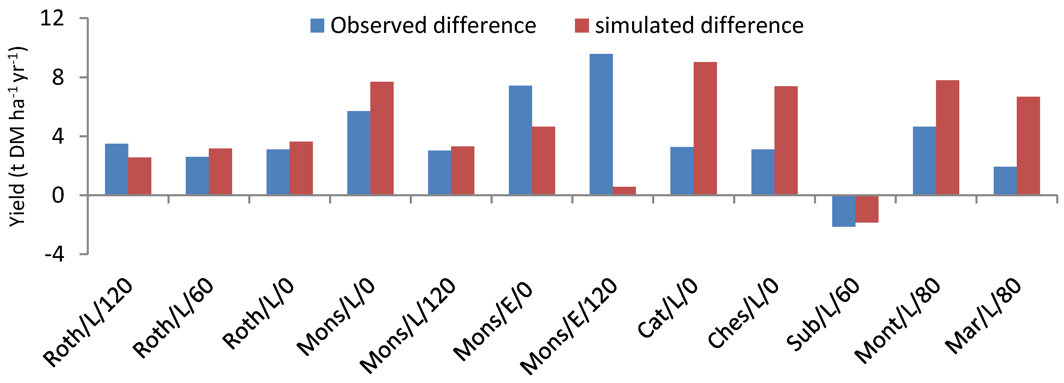
Adaptation to switchgrass. Except for the difference in base temperatures, all the above equations and concepts apply equally to miscanthus and switchgrass. For lack of similar literature and modeling concepts pertaining to switchgrass, the latter crop was modeled with the same equations, whether for crop development stages, photosynthesis or LAI development. The simulation of drought kill gave one exceptional major difference between the two crops. On any given year miscanthus was considered to fail if plant available water remained at zero for more than one month at a time (without compromising next year’s harvest), and the crop was terminated if this condition extended for more than two months [32]. This condition was deactivated for switchgrass, for which no such effects were reported, resulting in a higher tolerance to water stress for this crop.

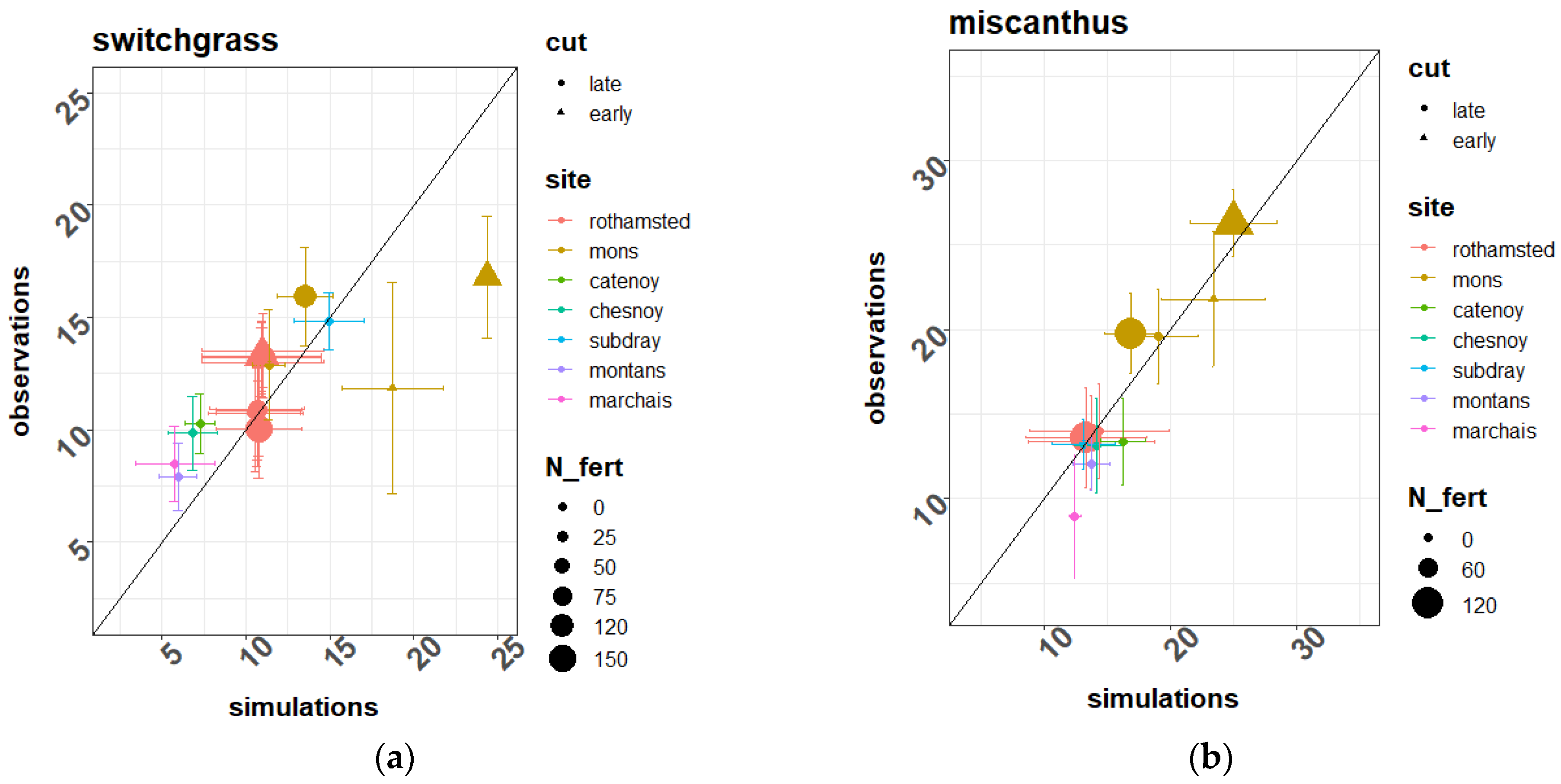
The parameters used to simulate the two crops on the Estrées-Mons site were mostly extracted from the literature, as can be seen in the Appendix A, Table A1.

Some of them (especially for switchgrass) were calibrated by fitting the model against the experimental data of this site. Such was the case for the radiation use efficiency, for example (Table A1). The selection of parameters undergoing such calibration (done by trial and error and for a single parameter at a time) was based on a preliminary sensitivity analysis of the times series of simulated biomass and crop N content.

2.2. Experimental Data

The Estrées-Mons dataset. The Estrées-Mons field trial was conducted from 2006 to 2015 in northern France (49°87′ N, 3°01′ E). It is part of a long-term experiment called “Biomass & Environment” [34,35]. The climate is temperate with oceanic influence, with a mean annual rainfall of 625 mm and a mean air temperature of 10.7 °C. The soil is a deep Haplic Luvisol with no major obstacles for root growth down to the 3 m depth. Miscanthus was planted in April 2006 at 1.5 rhizomes m⁻² and switchgrass (variety Kanlow) was sown in June 2006 at 15 kg seeds ha⁻¹. Both crops were harvested either in February–March (late harvest) or in October (early harvest) and two fertilization levels were compared for both crops, with input rates of 0 and 120 kg N ha⁻¹ yr⁻¹, respectively.

Several variables were measured for the various treatments implemented on this site, such as crop DM and N content in the different compartments of the plant [11,34] LAI, soil water and N contents over time [35].

The Rothamsted dataset. This field trial was conducted from 1998 to 2010 in southeastern UK (1°48′ N, 0°21′ W). The climate is oceanic, with a mean annual rainfall of 704 mm and a mean air temperature of 9°C. Switchgrass (variety Cave-in-rock) was planted in mid-April 1998. As in the Estrées-Mons site, switchgrass results are compared to miscanthus results from the same site and same period (

Table 1. Crop management characteristics for the experimental sites used for model calibration and testing.

3	Crop	Fertilizer N Rate (kg N ha−1 yr−1)	Irrigation	Harvest Dates	Timeframe
Estrées-Mons	Switchgrass	0/120	NO	early/late	2006–2015
Estrées-Mons	Miscanthus	0/120	NO	early/late	2006–2012
Rothamsted	Switchgrass	0/25/50/75/150	NO	early/late	1998–2010
Rothamsted	Miscanthus	0/60/120	NO	late	1993–2012
Marchais	switchgrass/miscanthus	80	NO	late	2008–2012
Montans	switchgrass/miscanthus	80	NO	late	2007–2013
Catenoy	switchgrass/miscanthus	0	NO	late	2006–2013
Subdray	switchgrass/miscanthus	60	First year	late	2008–2012
Chesnoy	switchgrass /miscanthus	0	First year	late	2006–2012

).

The measured variables at the Rothamsted site include time series of soil water and N contents, and final biomass yield. Unfortunately, no replicates were available for the measurements.

The Lignoguide network. This experimental network, originally comprising 9 sites across France, was set up as part of a research and development project aiming to help biomass growers make efficient and sustainable decisions regarding the choice of the most suitable crops. Here, we used data from 5 of these experimental sites that involved both miscanthus and switchgrass (cv. Kanlow): Catenoy, Chesnoy, Subdray, Marchais and Montans. Their main characteristics are summarized on Table 1 and

Table 2. Pedoclimatic and management characteristics of the Lignoguide experimental sites.

	Climatic Characteristics			Soil Type and Characteristics			Plant Available Water (mm)	Maximum Rooting Depth (cm)
	Climate Type	Mean Annual Rainfall (mm)	Mean Air Temperature (°C)	Soil Texture	CaCO3 Content (%)	Gravel Content (%)
Catenoy	Marine	446	13.9	Sandy loam	1%	0	150	100
Chesnoy	Marine	438	14.6	Sandy, stony and shallow	50% in the surface horizon.	20	55 to 75	50
Subdray	Marine	495	15	limestone-sandy	6% to 13%	10 to 25	125	60 to 80
Marchais	Marine	470	13.8	Sandy with 3% to 5% clay and 2% to 3% silt at the surface	9% to 13%	0	78	60
Montans	Mediterranean	471	16.8	Sandy loam	0.1%	15 to 40	43 mm for switchgrass	60 cm for switchgrass
							114 mm for miscanthus	80 cm for miscanthus

.

The measurements in the Lignoguide network concerned several variables, namely DM and N content in the different compartments of the plant, soil water and N contents over time.

2.3. Model Evaluation

The model was calibrated for miscanthus and switchgrass on the basis of experimental data from the Estrées-Mons site.

The model was subsequently tested on the other sites without modifying the equations or parameters. The model’s goodness of fit against the experimental data was assessed with the following statistical indicators:

-

Mean deviation:

$$MD=\frac{1}{n}{\displaystyle \sum }_{i=1}^n\left(predicted|i-observe{d}_i\right)$$

-

Root Mean Squared Error (RMSE):

$$RMSE={\sqrt{\frac{1}{n}{\displaystyle \sum }_{i=1}^n\left(predicte{d}_i-observe{d}_i\right)}}^2$$

-

rRMSE: a variant of the above measure, obtained by dividing RMSE by the average of the observed values.

3. Results

3.1. Model Calibration

Model calibration for the switchgrass at the Estrées-Mons data set proved difficult for some treatments, in particular the unfertilized controls. In the first years of the trial, crops responded very little to fertilizer N inputs (not shown), and this could not be mimicked by the model. According to the latter, soil N availability was clearly limiting biomass growth immediately following the establishment year. Although the soil was initially rich in inorganic N (with a stock around 200 kg N ha⁻¹ over the top 150 cm of soil), it was quickly depleted according to both the soil N measurements and the model simulations of soil N dynamics. Other aspects were difficult to calibrate: the rhizome dynamics over the growing seasons and years, especially in terms of nitrogen content, and carbon and N translocation from the rhizome to the aboveground parts of the plant (see following section and Figure 1 and Figure 2, depicting the final model results).

The best-fit values for the parameters that required calibration are listed in Appendix A, while

Table 3. Goodness of fit statistics for the simulation of the switchgrass crop.

	Aboveground Dry Matter Biomass					Final Aboveground Dry Matter Yield		Soil Mineral Nitrogen		Soil Water
	Calibration				Calibration	Validation	Global	Top Layer	Deep Layers	Top Layer	Deep Layers
	Early Harvest		Late Harvest
	Unfertilised	Fertilised	Unfertilised	Fertilised
Unit	t DM ha−1	t DM ha−1	t DM ha−1	t DM ha−1	t DM ha−1 yr−1	t DM ha−1 yr−1	t DM ha−1 yr−1	kg NO3-N ha−1	kg NO3-N ha−1	%	%
N: number of individuals	12	12	16	21	23	76	100	28	84	28	84
Mean Deviation	−0.17	−0.95	−0.80	−0.56	−0.34	−0.93	−0.78	−9.18	1.64	−0.21	0.14
RMSE	2.66	2.65	2.68	3.27	5.30	3.42	4.00	20.33	9.33	2.95	1.90
rRMSE	34	21	27	28	21	30	33	95	98	8	6

and

Table 4. Goodness of fit statistics for the simulation of the miscanthus crop.

	Aboveground Dry Matter Biomass					Final Dry Matter Yield		Soil Nitrogen		Soil Water
	Calibration				Calibration	Testing	Global	Topsoil	Deep Layers	Topsoil	Deep Layers
	Early Harvest		Late Harvest
	Unfertilized	Fertilized	Unfertilized	Fertilized
Unit	t DM ha−1	t DM ha−1	t DM ha−1	t DM ha−1	t DM ha−1 yr−1	t DM ha−1 yr−1	t DM ha−1 yr−1	kg NO3-N ha−1	kg NO3-N ha−1	%	%
N: number of individuals	12	12	16	21	23	76	100	17	51	16	48
Mean Deviation	−0.30	4.23	−0.13	2.70	−2.16	0.57	0.04	−12.62	−5.04	−0.53	−2.90
RMSE	3.30	4.77	3.54	4.30	4.69	4.74	4.73	13.86	13.50	3.02	4.60
rRMSE	23	38	21	29	37	35	31	83	193	8	14

provide statistical indicators on the model’s goodness of fit in the calibration and evaluation phases.

3.2. Model Evaluation in the Calibration Site

3.2.1. Plant Biomass

Figure 1 compares the dynamics of simulated and observed plant biomass for the miscanthus crop in Estrées-Mons, in the various plant compartments (leaf, stems and rhizomes) throughout its growing cycle.

For miscanthus, during the first years of cultivation (up to 2011), the model gave correct estimates for the build-up of biomass in the rhizomes, senescent and green leaves, but overestimated stem biomass for the fertilized treatments (with a mean deviation (MD) of 4.23 t DM ha⁻¹ for the late cut) and underestimated it for the unfertilized controls (with a MD of −0.3 t DM ha⁻¹ for the late cut).

Similar to miscanthus, the model adequately captured the time variations of biomass in the plant compartments (rhizome and leaves) for switchgrass (Figure 2). An underestimation of stem biomass during the growing season is noticeable during the first years of the cultivation cycle for all treatments, as is a strong overestimation of the biomass of green leaves upon harvest for the early cuts.

For all treatments and crops, the model captured the intra-annual dynamics of the aboveground biomass, which increased from spring to autumn and slightly decreased thereafter as a result of translocation to the rhizomes (visible on Figure 1 and Figure 2). The effect of inter-annual variability is also noticeable on Figure 2, with yields varying between 12 and 14 t DM ha⁻¹ for the unfertilized and late harvest treatments, for instance for switchgrass. This translates the response of the plant to climatic conditions, which the model was able to mimic to some extent: for all treatments, simulated and observed yields varied within a similar range, but for some years (such as 2010) the model over-estimated the harvested biomass of the fertilized switchgrass by 1 to 6 t DM ha⁻¹. Regarding the establishment phase, the second year of the switchgrass crop (corresponding to the first year depicted in Figure 1) was characterized by very low simulated yields, especially for the unfertilized crops.

The model responded significantly to the four management treatments tested for switchgrass and miscanthus. Although it tended to underestimate the biomass of unfertilized crops (see the sub-section on calibration), the model proved more successful in simulating the overwinter loss of aboveground biomass associated with the late cuttings, which took place in February. This decrease is due to translocation to the rhizomes, at the end of the growing season.

3.2.2. Nitrogen Partitioning in the Plant

Figure 3 compares the observed and simulated amounts of nitrogen in the above- and below-ground parts of the plant over time. As perennial plants, miscanthus and switchgrass are characterized by seasonal displacements of N in relation to their development stage, similar to the biomass translocation and remobilization fluxes described in the above section. However, it should be noted that N translocation or remobilization flows are calculated independently of biomass fluxes, using different drivers and source/sink concepts altogether. Over the years, there appeared a growing discrepancy between the observed and simulated rhizome N contents, especially with the fertilized treatments.

The translocation of N from the aerial to below-ground plant parts at the end of the growing season was apparent in the decline of shoot N content (according to the simulations, and a few experimental samplings taken during the growing season), while the remobilization of N in the spring caused a decrease of rhizome N stocks. This was also visible in the measured data points for the year 2015 (Figure 3). According to the model, this pattern of decrease and increase for the rhizome N pool was more pronounced with the fertilized crop, whereas it hardly appeared in the simulation of the unfertilized control for both crops. This is somewhat surprising, but may be due to the fact that remobilization in spring was constrained by a minimum N concentration imposed in the rhizome biomass, which was rarely exceeded—reducing, in effect, the quantity of translocatable N to zero. Unfortunately, adjusting this threshold N content did not improve the simulations overall.

The effect of fertilizer input was notable in the simulations: the rhizomes accumulated much more N in this case than with the unfertilized control, with about a three-fold difference in rhizome N after 10 years (Figure 3). This explains why biomass was underestimated for the unfertilized control, for which the only way to reach biomass production levels close to the observed ones involved increasing the soil N mineralization rates, by changing the initial soil organic C and N levels. Since this calibration had little to do with the real conditions of the experiment, it was not pursued any further.

3.2.3. Soil Nitrogen and Water Dynamics

Figure 4 depicts the simulated versus observed dynamics of soil water and mineral nitrogen contents in the various soil layers for a fertilized switchgrass crop in Estrée-Mons. In the topsoil, the simulated soil N content spiked every year after the application of mineral fertilizer N in spring. Since soils were sampled prior to this event or several months afterward, it is difficult to verify the pattern of sharp decrease following fertilization. However, the model achieved an overall RMSE of 9.3 kg NO₃-N ha⁻¹ (Table 3) across all treatments for the sub-soil layers (under the 30 cm depth), and of 20 kg NO₃-N ha⁻¹ for the topsoil. For the sub-soil layers, soil N was highly over-estimated (mean deviation of 9.2 kg NO₃-N ha⁻¹ (Table 3)) and the observed seasonal dynamics were less pronounced altogether, with relatively low levels of mineral N throughout.

The model simulated the depletion of soil water content in spring through summer due to plant evapo-transpiration, as well as its recharge in autumn through winter, in accordance with the measurements taken during the 2015 growing season (Figure 4). For the deeper layers, simulations of soil water dynamics for switchgrass were in good agreement with the measurements (with a RSME of 1.9% (v/v) and a mean deviation of 0.14%; Table 3).

3.3. Model Testing

Figure 5 compares the simulated and observed yields across the six testing sites for switchgrass and miscanthus, and also includes the Estrées-Mons calibration site. For the miscanthus crop, most points are close to the 1:1 line, falling within 1–3 t DM ha⁻¹ from the observations. This resulted in a relatively low mean deviation (of 0.04 t DM ha⁻¹) and a relative RMSE of 31% overall (Table 4). For the switchgrass crop, most points on Figure 5 were located on the upper half of the graph, pointing to a tendency of the model to underestimate biomass production. The observed miscanthus yields were consistently higher than those for switchgrass, ranging from 11 t DM ha⁻¹ to 26 t DM ha⁻¹, in comparison with a 7–15 t DM ha⁻¹ range for switchgrass.

Overall, the model managed to capture the variations in miscanthus and switchgrass yields across the various sites and treatments, with mean deviations under 1% of the average yields, and global RMSEs of 4.7 t DM ha⁻¹ for miscanthus and 4 t DM ha⁻¹ for switchgrass. This translates as relative RMSEs of 31% and 33%, respectively (Table 4).

Figure 6 provides a visual assessment of the model’s overall ability to capture the differences between the time-averaged yields of miscanthus and switchgrass across the various sites and treatments tested here. For the observations, as well as the simulations, yields were higher for miscanthus, except for the Subdray site where switchgrass performed slightly better than miscanthus. This was due to the shallow soil conditions occurring there, resulting in a larger water stress for miscanthus over the years. The model ranked the crops correctly for all sites and treatments, with gaps that were most of the time lower than the RMSE achieved by the models for the individual crops (under 4 t DM ha⁻¹).

In terms of goodness of fit statistics, the model achieved a mean deviation of 0.46 t DM ha⁻¹ in its prediction of the yield differences (

Table 5. Statistical analyses of the difference between the yields of miscanthus and switchgrass crops.

	Yield Difference (Between Miscanthus and Switchgrass)
	t DM ha−1 yr−1
N: number of individuals	12
Mean Deviation	0.46
RMSE	3.65
rRMSE	135%

), which was higher than that for the yields of single crops, but much lower than the individual yield gaps themselves. The RMSE was also similar to those achieved with the single crop yields (at 3.65 t DM ha⁻¹), and was in the lower end of the yield gaps.

4. Discussion

The original aim of this piece of work was to calibrate the CERES-EGC model for two perennial crops (miscanthus and switchgrass), and to assess whether this biophysical model was capable of capturing the differences of biomass yields between these crops across a range of pedoclimatic conditions. The model was also tested regarding its response to crop management practices. This appeared as a pre-requisite of such models being used to aid the selection of candidate feedstocks in a given local context and assess their environmental performances.

According to the results obtained in the seven experimental situations tested here with CERES-EGC, it appears that this model did grasp the differences between miscanthus and switchgrass across the locations it attempted, achieving an overall MD of 0.46 t DM ha⁻¹. It provided a correct ranking of the crops, in line with the literature, where miscanthus is found to be more productive than switchgrass [25,27]. Its yield simulations came with a relative error of 31% (as estimated by the RMSE). This margin is probably higher than the field variability typically encountered when measuring the biomass of perennial crops, and is significantly larger when calculated with the measurement errors associated with their estimation, in particular for crop yields. This implies that a biophysical model, such as CERES-EGC, could be a valuable tool for benchmarking candidate feedstocks, as hypothesized at the start of this study. We are not aware of previous work aiming at comparing the performance of crops to observations, and therefore we may only compare the prediction error of CERES-EGC to studies focusing on single crops. The RMSE obtained here for miscanthus yields (4.7 t DM ha⁻¹) is comparable to that calculated for the same crop with the STICS model, which achieved a RMSE of 3.4 t DM ha⁻¹ [36].For the switchgrass, the RMSE calculated here is 4 t DM ha⁻¹, which corresponds to what is found on average in the literature, where the values of RMSE vary from 2.7 t DM ha⁻¹ [37] to 6.54 t DM ha⁻¹. Overall, the relative RMSE values (ranging from 31% to 33%) are of the higher end of the results from the simulation of annual arable crops with the STICS model [26].

It may be argued that it is easier to simulate the yield differences between two crops than their individual yields, since possible bias in absolute terms for single crops may cancel each other out when computing the yield differences between them. However, in this exercise, the mean deviation and RMSE values were actually higher for the yield difference than the single yields, showing that these differences are still more difficult to capture than variations in the crop yields across sites and treatments. Still, the model managed a correct ranking of the crops’ biomass production levels in all the cases in which it attempted it.

The model responded to the different pedoclimatic conditions encountered in the field trials, with higher yields for sites with higher rainfall (e.g., Estrées-Mons or Rothamsted). The Estrées-Mons site was also characterized by a high soil nitrogen availability, which supplied large amounts of N to the unfertilized control crops, enabling them to reach yield levels close to their fertilized counterparts. Conversely, the model also predicted very low yields for shallow soils. This was the case for the Subdray site, with a shallow rooting depth (of 60 cm only), which achieved the lowest observed yields for miscanthus and switchgrass.

In principle, it is much easier to predict data for an experimental site in which the model is calibrated. When the parameters are properly adjusted, the RMSE would be close to the ‘minimum’ prediction error that the model can achieve given its intrinsic (structural) lack of accuracy [38]. Here, the model was calibrated on one site (Estrées-Mons) and tested on six other sites. Because of the difficulties encountered in the calibration phase, especially in view of a trade-off between the early years of the crops and their later stages, the RMSE values were similar between the calibration and testing phases for miscanthus, and actually better in the second phase for switchgrass (3.42 DM ha⁻¹ vs. 5.30 t DM ha⁻¹ for the calibration set). It may be concluded that the calibrated parameters obtained in one location did apply to a wider range of pedoclimatic conditions, as observed at the six testing sites, and may be used in a broader range of contexts. However, the Estrée-Mons data set was also much more elaborate, in that it involved data on soil N and crop N dynamics and all treatments, providing insight into the relevance of the modeling concepts and principles. The relatively low prediction capacity of CERES-EGC for this trial points to a difficulty in correctly representing N translocation processes and storage in the below-ground plant compartments.

As a consequence, the simulation of the remobilization between belowground and aerial parts should be improved. As it currently stands, the model simulates both translocation and remobilization, but it tends to accumulate too much nitrogen in the rhizome (Figure 4). Since the model does not incorporate an age factor per se (assuming this should be consequence of rhizome dynamics), it is difficult to conclude that it can account for the yield decline observed in Estrées-Mons over all the treatments for switchgrass. In particular, the model failed to account for the low yields observed in the final year of the trial (2016), with values under 10 t DM ha⁻¹ for all treatments. It may arise from the large underestimation of the rhizome N pool for the unfertilized crops, but this error did not apply to the fertilized treatments. For these crops, this decline may be related to the plantation’s age.

As a conclusion, the CERES-EGC model may be used to rank two major candidate crops for lignocellulose production, in response to pedoclimatic conditions and also crop management practices, to some extent. In a further step, coupling this model with an economic model would make it possible to quantify the competitive advantages of these two crops at the level of a region or a country in Europe.

References

1. IPCC. Summary for Policymakers. In IPCC Special Report on Renewable Energy Sources and Climate Change Mitigation; Edenhofer, O., Pichs-Madruga, R., Sokona, Y., Seyboth, K., Matschoss, P., Kadner, S., Zwickel, T., Eickemeier, P., Hansen, G., Schlömer, S., et al., Eds.; Cambridge University Press: Cambridge, UK; New York, NY, USA, 2011. [Google Scholar]
2. Mohr, A.; Raman, S. Lessons from first generation biofuels and implications for the sustainability appraisal of second generation biofuels. Energy Policy 2013, 63, 114–122. [Google Scholar] [CrossRef] [PubMed]
3. European Parliament. Directive (EU) 2015/1513 of the European Parliament and of the Council of 9 September 2015 Amending Directive 98/70/EC Relating to the Quality of Petrol and Diesel Fuels and Amending Directive 2009/28/EC on the Promotion of the Use of Energy from Renewable Sources. Available online: https://eur-lex.europa.eu/legal-content/EN/TXT/?uri=celex%3A32015L1513 (accessed on 20 July 2020).
4. Havlík, P.; Schneider, U.A.; Schmid, E.; Böttcher, H.; Fritz, S.; Skalský, R.; Aoki, K.; Cara, S.D.; Kindermann, G.; Kraxner, F.; et al. Global land-use implications of first and second generation biofuel targets. Energy Policy 2011, 39, 5690–5702. [Google Scholar] [CrossRef]
5. El Akkari, M.; Réchauchère, O.; Bispo, A.; Gabrielle, B.; Makowski, D. A meta-analysis of the greenhouse gas abatement of bioenergy factoring in land use changes. Sci. Rep. 2018, 8, 1–7. [Google Scholar] [CrossRef] [PubMed]
6. Lesur, C.; Jeuffroy, M.-H.; Makowski, D.; Riche, A.B.; Shield, I.; Yates, N.; Fritz, M.; Formowitz, B.; Grunert, M.; Jorgensen, U.; et al. Modeling long-term yield trends of Miscanthus×giganteus using experimental data from across Europe. Field Crops Res. 2013, 149, 252–260. [Google Scholar] [CrossRef]
7. Lewandowski, I.; Heinz, A. Delayed harvest of miscanthus—Influences on biomass quantity and quality and environmental impacts of energy production. Eur. J. Agron. 2003, 19, 45–63. [Google Scholar] [CrossRef]
8. Cadoux, S.; Riche, A.B.; Yates, N.E.; Machet, J.-M. Nutrient requirements of Miscanthus x giganteus: Conclusions from a review of published studies. Biomass Bioenergy 2012, 38, 14–22. [Google Scholar] [CrossRef]
9. Wright, L.; Turhollow, A. Switchgrass selection as a “model” bioenergy crop: A history of the process. Biomass Bioenergy 2010, 34, 851–868. [Google Scholar] [CrossRef]
10. Amougou, N.; Bertrand, I.; Cadoux, S.; Recous, S. Miscanthus × giganteus leaf senescence, decomposition and C and N inputs to soil. GCB Bioenergy 2012, 4, 698–707. [Google Scholar] [CrossRef]
11. Strullu, L.; Cadoux, S.; Preudhomme, M.; Jeuffroy, M.H.; Beaudoin, N. Biomass production and nitrogen accumulation and remobilisation by Miscanthus x giganteus as influenced by nitrogen stocks in belowground organs. Field Crops Res. 2011, 121, 381–391. [Google Scholar] [CrossRef]
12. Drewer, J.; Finch, J.W.; Lloyd, C.R.; Baggs, E.M.; Skiba, U. How do soil emissions of N2O, CH4 and CO2 from perennial bioenergy crops differ from arable annual crops? GCB Bioenergy 2012, 4, 408–419. [Google Scholar] [CrossRef] [Green Version]
13. Gauder, M.; Butterbach-Bahl, K.; Graeff-Hönninger, S.; Claupein, W.; Wiegel, R. Soil-derived trace gas fluxes from different energy crops—Results from a field experiment in Southwest Germany. GCB Bioenergy 2012, 4, 289–301. [Google Scholar] [CrossRef]
14. Nsanganwimana, F.; Pourrut, B.; Mench, M.; Douay, F. Suitability of Miscanthus species for managing inorganic and organic contaminated land and restoring ecosystem services. A review. J. Environ. Manag. 2014, 143, 123–134. [Google Scholar] [CrossRef] [PubMed]
15. Scordia, D.; Testa, G.; Cosentino, S.L. Perennial grasses as lignocellulosic feedstock for second-generation bioethanol production in Mediterranean environment. Ital. J. Agron. 2014, 9, 84. [Google Scholar] [CrossRef]
16. Feng, Q.; Chaubey, I.; Engel, B.; Cibin, R.; Sudheer, K.P.; Volenec, J. Marginal land suitability for switchgrass, Miscanthus and hybrid poplar in the Upper Mississippi River Basin (UMRB). Environ. Model. Softw. 2017, 93, 356–365. [Google Scholar] [CrossRef] [Green Version]
17. Izaurralde, R.C.; McGill, W.B.; Williams, J.R.; Jones, C.D.; Link, R.P.; Manowitz, D.H.; Schwab, D.E.; Zhang, X.; Robertson, G.P.; Millar, N. Simulating microbial denitrification with EPIC: Model description and evaluation. Ecol. Model. 2017, 359, 349–362. [Google Scholar] [CrossRef]
18. Lee, J.; Pedroso, G.; Linquist, B.A.; Putnam, D.; Kessel, C.; Six, J. Simulating switchgrass biomass production across ecoregions using the DAYCENT model. GCB Bioenergy 2012, 4, 521–533. [Google Scholar] [CrossRef]
19. Wagena, M.B.; Bock, E.M.; Sommerlot, A.R.; Fuka, D.R.; Easton, Z.M. Development of a nitrous oxide routine for the SWAT model to assess greenhouse gas emissions from agroecosystems. Environ. Model. Softw. 2017, 89, 131–143. [Google Scholar] [CrossRef] [Green Version]
20. Peyrard, C.; Ferchaud, F.; Mary, B.; Gréhan, E.; Léonard, J. Management Practices of Miscanthus × giganteus Strongly Influence Soil Properties and N2O Emissions Over the Long Term. BioEnergy Res. 2017, 10, 208–224. [Google Scholar] [CrossRef]
21. Strullu, L.; Beaudoin, N.; de Cortàzar Atauri, I.G.; Mary, B. Simulation of Biomass and Nitrogen Dynamics in Perennial Organs and Shoots of Miscanthus × Giganteus Using the STICS Model. BioEnergy Res. 2014, 7, 1253–1269. [Google Scholar] [CrossRef]
22. Gabrielle, B.; Gagnaire, N.; Massad, R.S.; Dufossé, K.; Bessou, C. Environmental assessment of biofuel pathways in Ile de France based on ecosystem modeling. Bioresour. Technol. 2014, 152, 511–518. [Google Scholar] [CrossRef] [PubMed] [Green Version]
23. Heaton, E.A.; Dohleman, F.G.; Long, S.P. Meeting US biofuel goals with less land: The potential of Miscanthus. Glob. Chang. Biol. 2008, 14, 2000–2014. [Google Scholar] [CrossRef]
24. Gelfand, I.; Shcherbak, I.; Millar, N.; Kravchenko, A.N.; Robertson, G.P. Long-term nitrous oxide fluxes in annual and perennial agricultural and unmanaged ecosystems in the upper Midwest USA. Glob. Chang. Biol. 2016, 22, 3594–3607. [Google Scholar] [CrossRef] [PubMed]
25. Iqbal, Y.; Gauder, M.; Claupein, W.; Graeff-Hönninger, S.; Lewandowski, I. Yield and quality development comparison between miscanthus and switchgrass over a period of 10 years. Energy 2015, 89, 268–276. [Google Scholar] [CrossRef]
26. Coucheney, E.; Buis, S.; Launay, M.; Constantin, J.; Mary, B.; García de Cortázar-Atauri, I.; Ripoche, D.; Beaudoin, N.; Ruget, F.; Andrianarisoa, K.S.; et al. Accuracy, robustness and behavior of the STICS soil–crop model for plant, water and nitrogen outputs: Evaluation over a wide range of agro-environmental conditions in France. Environ. Model. Softw. 2015, 64, 177–190. [Google Scholar] [CrossRef]
27. Laurent, A.; Pelzer, E.; Loyce, C.; Makowski, D. Ranking yields of energy crops: A meta-analysis using direct and indirect comparisons. Renew. Sustain. Energy Rev. 2015, 46, 41–50. [Google Scholar] [CrossRef]
28. Mann, J.J.; Barney, J.N.; Kyser, G.B.; DiTomaso, J.M. Root System Dynamics of Miscanthus × giganteus and Panicum virgatum in Response to Rainfed and Irrigated Conditions in California. BioEnergy Res. 2013, 6, 678–687. [Google Scholar] [CrossRef]
29. Davis, S.C.; Parton, W.J.; Dohleman, F.G.; Smith, C.M.; Grosso, S.D.; Kent, A.D.; DeLucia, E.H. Comparative Biogeochemical Cycles of Bioenergy Crops Reveal Nitrogen-Fixation and Low Greenhouse Gas Emissions in a Miscanthus × giganteus Agro-Ecosystem. Ecosystems 2010, 13, 144–156. [Google Scholar] [CrossRef]
30. Jones, C.A.; Kiniry, J.R.; Dyke, P.T. CERES-Maize: A Simulation Model of Maize Growth and Development; Texas A&M University Press: College Station, TX, USA, 1986. [Google Scholar]
31. Gabrielle, B.; Laville, P.; Hénault, C.; Nicoullaud, B.; Germon, J.C. Simulation of Nitrous Oxide Emissions from Wheat-cropped Soils using CERES. Nutr. Cycl. Agroecosystems 2006, 74, 133–146. [Google Scholar] [CrossRef] [Green Version]
32. Hastings, A.; Clifton-Brown, J.; Wattenbach, M.; Mitchell, C.P.; Smith, P. The development of MISCANFOR, a new Miscanthus crop growth model: Towards more robust yield predictions under different climatic and soil conditions. Glob. Chang. Biol.Bioenergy 2009, 1, 154–170. [Google Scholar] [CrossRef]
33. Heaton, E.A.; Dohleman, F.G.; Long, S.P. Seasonal nitrogen dynamics of Miscanthus × giganteus and Panicum virgatum. GCB Bioenergy 2009, 1, 297–307. [Google Scholar] [CrossRef]
34. Cadoux, S.; Ferchaud, F.; Demay, C.; Boizard, H.; Machet, J.M.; Fourdinier, E.; Preudhomme, M.; Chabbert, B.; Gosse, G.; Mary, B. Implications of productivity and nutrient requirements on greenhouse gas balance of annual and perennial bioenergy crops. Glob. Chang. Biol. Bioenergy 2014, 6, 425–438. [Google Scholar] [CrossRef]
35. Ferchaud, F.; Mary, B. Drainage and Nitrate Leaching Assessed During 7 Years Under Perennial and Annual Bioenergy Crops. BioEnergy Res. 2016, 9, 656–670. [Google Scholar] [CrossRef]
36. Strullu, L.; Ferchaud, F.; Yates, N.; Shield, I.; Beaudoin, N.; Garcia de Cortazar-Atauri, I.; Besnard, A.; Mary, B. Multisite Yield Gap Analysis of Miscanthus × giganteus Using the STICS Model. BioEnergy Res. 2015, 8, 1735–1749. [Google Scholar] [CrossRef]
37. Brown, R.A.; Rosenberg, N.J.; Hays, C.J.; Easterling, W.E.; Mearns, L.O. Potential production and environmental effects of switchgrass and traditional crops under current and greenhouse-altered climate in the central United States: A simulation study. Agric. Ecosyst. Environ. 2000, 78, 31–47. [Google Scholar] [CrossRef] [Green Version]
38. Wallach, D. Crop Model Calibration: A Statistical Perspective. Agron. J. 2011, 103, 1144. [Google Scholar] [CrossRef]
39. Strullu, L. Nitrogen Fluxes in a Perennial Energetic Crop, Miscanthus × Giganteus: Experimental Study and Modelling Elements. Ph.D. Thesis, AgroParisTech, Paris, France, 2011. [Google Scholar]
40. Miguez, F.E.; Zhu, X.; Humphries, S.; Bollero, G.A.; Long, S.P. A semimechanistic model predicting the growth and production of the bioenergy crop Miscanthus × giganteus: Description, parameterization and validation. GCB Bioenergy 2009, 1, 282–296. [Google Scholar] [CrossRef]
Figure 1. simulated (lines) and observed (symbols) dynamics of biomass in various plant compartments for the miscanthus trial in the Estrées-Mons calibration site, and for four treatments combining late and early harvests with two levels of N fertilizer inputs (0 and 120 kg N ha−1).
Energies 13 03942 g001
Figure 2. simulated (lines) and observed (symbols) dynamics of biomass in various plant compartments for the switchgrass trial in the Estrées-Mons calibration site, and for four treatments combining late and early harvests with two levels of N fertilizer inputs (0 and 120 kg N ha−1).
Energies 13 03942 g002
Figure 3. Simulated (lines) and observed (symbols) dynamics of nitrogen in the above and below-ground plant compartments for two treatments of the switchgrass and miscanthus crops in Estrées-Mons.
Energies 13 03942 g003
Figure 4. Soil mineral nitrogen (top) and soil water (bottom) dynamics for miscanthus early harvest without fertilization (a) and switchgrass late harvest with fertilization (b) in Estrée-Mons (the label of the y axis is indicated on the right hand side of the graphs).
Energies 13 03942 g004
Figure 5. Simulated vs. observed yields for the (a) switchgrass and (b) miscanthus crops across the 7 experimental sites and management treatments. Symbols represent the average yields over the lifespan of the crops, and are coded according to the location and management treatments of these experiments. The error bars represent the standard deviations of the same series of simulated and observed yields for each site-treatment combination. Key to variables: cut—harvest time (late or early); N_fert—Fertiliser N input rate (kg N ha−1 yr−1).
Energies 13 03942 g005
Figure 6. Histogram of differences between miscanthus and switchgrass annual yields, as observed (blue bars) or simulated by CERES-EGC (red bars) across the different experimental sites Rothamsted (Roth), Estrée-Mons (Mons), Catenoy (cat), Chesnoy (CHes), Subdray (Sub), Montant (Mont) and Marchais (Mar). For each region the difference is calculated for each cut (late (L) and early (E)), and each fertilization level (0, 60, 80 or 120 kg N ha−1 yr−1).
Energies 13 03942 g006