A Conceptual Framework to Describe Energy Efficiency and Demand Response Interactions

Abstract

Energy efficiency (EE) and demand response (DR) resources provide important utility systems and ratepayer benefits. At the same time, the rapid change in the amount and type of variable renewable energy, like solar and wind, is reshaping the role and economic value of EE and DR, and will likely affect the time-dependent valuation of EE and DR measures. Utilities are increasingly interested in integrating EE and DR measures as a strategic approach to improve their collective cost-effectiveness and performance. We develop a framework to identify the EE and DR attributes, system conditions, and technological factors that are likely to drive interactions between EE and DR. We apply the framework to example measures with different technology specifics in the context of different utility system conditions. We find that EE and DR interactions are likely driven by changes in discretionary load, the addition of controls or other capabilities to shift loads, and the coincidence of savings with system peak or load building periods. Our analysis suggests increasing complexity in evaluating EE and DR interactions when moving from standalone equipment to integrated systems. The framework can be applied to research on integrated building systems by grouping measures into portfolios with different likely implications for EE and DR interactions.

1. Introduction

Integrating energy efficiency (EE) and demand response (DR) can drive significant reductions in electricity use and greenhouse gas emissions in the building sector, as well as provide important utility systems and ratepayer benefits. The benefits include reducing and/or shifting load to increase system capacity factors or to facilitate economic or security-constrained dispatch of generation resources [1,2,3,4]; deferral of generation, transmission, and distribution system investments [5]; and reductions in fuel and purchased power costs for utilities and end-users of electricity [6]. In addition, EE programs typically cost less per kilowatt-hour than average retail electricity rates [7,8,9] and can provide substantial CO₂ emissions reductions [10].

At the same time, the rapid change in the amount and type of variable renewable energy (VRE), like solar and wind, is reshaping the role and economic value of EE and DR. The proliferation of distributed generation (DG) has reduced utility retail sales and changed the timing of net peak demand. Additionally, the diurnal patterns and volatility of wholesale prices are changing due, in part, to large increases in utility-scale renewable generation resources with zero marginal costs [11]. These changes will likely affect the time-dependent valuation of EE and DR measures [12]. In some cases, EE and DR resources by themselves may no longer be cost-effective on the basis of cost avoidance alone as marginal energy costs decline [13]. Utilities are increasingly interested in integrating EE and DR measures and technologies (as well as other distributed energy resources) as a strategic approach to improve their collective cost-effectiveness [14,15].

Integrating EE and DR is an emerging research area with limited implementation experience [14,15]. Prior studies on EE and DR interactions and integration have focused primarily on institutional and market barriers [16], driving customer acceptance and participation [17,18], implementing behavior-based programs targeting EE and DR goals [19], and optimizing EE and DR resource benefits [1,20,21]. We develop a conceptual framework to fill literature gaps regarding which specific EE and DR features may be best suited for integration, the interplay between changing EE and DR resource potential, and resulting utility system impacts. Specifically, this research identifies the EE and DR attributes, system conditions, and technological factors that are likely to drive interactions between EE and DR. Understanding the distinct characteristics of EE and DR resources (e.g., temporal savings, flexibility) can inform the interactive role of EE and DR combined to optimize DF in future electricity systems with greater adoption of VRE and distributed energy resources (DERs), including DG, storage, and electric vehicles.

The framework focuses primarily on system impacts from the perspective of the utility or system operator. We consider the customer perspective, to a lesser extent, as part of assessing the change in the load that is available to provide demand flexibility (DF), defined as the capability associated with a building to modify energy consumption in response to utility grid needs [22]. We do not explore changes in customer economics (e.g., bill savings resulting in changes to payback period), customer perceptions of or attitudes towards EE or DR (e.g., through increased awareness of energy consumption patterns), broader policy issues of utility financial impacts (e.g., changes in utility collected revenues, achieved earnings, and achieved return-on-equity), or the alignment (or lack thereof) between program design and retail and wholesale market opportunities. However, we acknowledge that these are important factors for utilities and decision-makers to consider. Last, we follow the typical practice to define EE and DR as separate resources. Regulators have historically authorized separate ratepayer funding streams for EE and DR programs. Partially as a result, utilities and program administrators design, plan, and enroll participants for EE and DR programs separately [14,16].

2. Materials and Methods

2.1. Definitions

EE and DR differ from each other in ways that are important for understanding how EE and DR interact and are applied in the conceptual framework. We define EE as a persistent and maintained reduction in building energy consumption required to provide a fixed level of service, which is consistent with other definitions [16,23]. By contrast, we define DR as an active modification in building energy demand or consumption on a limited-time basis, in response to a financial incentive or command signal, which may result in a reduced level of service. From the utility perspective, DR resources are used by system operators for economic (e.g., high wholesale electricity prices) benefits or during reliability (e.g., high load or capacity shortage) events and the frequency and duration of such events can vary greatly from one year to another [24]. In many cases, utility DR programs limit the number of hours that customers can be called to provide DR resources [16]. Therefore, in practice, DR is a more circumscribed resource whose use is contingent on actual system needs that transpire in or near real-time. Like DR, DF is characterized by active load management on timescales consistent with utility system and grid needs. Unlike EE and DR, DF is not a resource in the traditional sense, but a potential that the utility or system operator can utilize to provide reliable electricity service.

2.2. Conceptual Framework

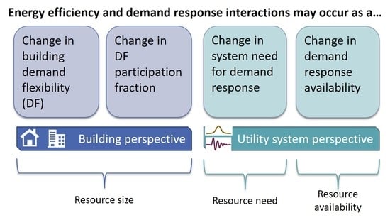
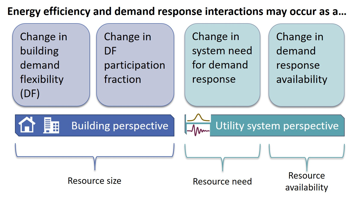
The framework describes the interactive effects of a “change,” which is defined by the point at which an EE or DR investment is made by a residential customer, commercial customer, or aggregator operating across multiple buildings. The framework is comprised of two levels, each of which is subdivided further into two sublevels exploring one of the four interactions that may occur between EE and DR (see

Table 1. Framework levels, change metrics, and definitions of competition, complementarity, and neutral interactions between energy efficiency (EE) and demand response (DR).

Level	Perspective	Change Metric	EE and DR Interactions
			Competition	Complementarity	Neutral
1a	Building	DF	Less loadable to shed, shift, or modulate	More loadable to shed, shift, or modulate	No change in loadable to shed, shift, or modulate
1b	Building	DF participation fraction	Lower fraction of DF participating as a demand response resource	Higher fraction of DF participating as a demand response resource	No change in the fraction of DF participating as a demand response resource
2a	Utility system	Demand response (DR) 1 need	Increased likelihood of needing DR resources to meet utility system conditions	Decreased likelihood of needing DR resources to meet utility system conditions	No change in the likelihood of needing DR resources to meet utility system conditions
2b	Utility system	DR availability	Reduced availability of DR resources to meet specific system need or condition	Increased availability of DR resources to meet specific system need or condition	No change in the availability of DR resources to the system operator

¹ The focus on DR resources in Levels 2a and 2b is consistent with the characterization of DR as a dispatchable resource (as compared to EE) by utility system operators. The impacts and resultant value of EE at the utility system in levels 2a and 2b are captured by the size and timing of its reductions in utility system load.

).

The first level assesses changes that occur at the building and across two sources of EE and DR interactions. At level 1a, interactions may occur when an EE investment increases (complements) or decreases (competes with) the size of the available DR resource. At level 1b, EE upgrades might encourage more (complementary) or less (competing) participation in DR programs with the affected load. It is also possible that no change occurs as illustrated by a neutral interaction.

The second level aggregates buildings to represent utility-scale changes across two sources of EE and DR interactions. At level 2a, an increase in EE may either decrease (complement) or increase (compete with) the system need for DR resources to balance real-time utility grid supply and demand. At level 2b, utility system operators use DR resources to meet grid needs, including for capacity and energy requirements and ancillary services (e.g., frequency regulation, spinning and non-spinning reserves). EE and DR interact in terms of resource availability when an EE measure applied widely in the building stock either increases (complements) or decreases (competes with) the availability of DR resources. Again, should no change occur, then a neutral designation is applied.

For each sublevel, we identify the metric by which the interaction between EE and DR is measured. We assess interactions across three different types of DF and DR: (1) peak shed (i.e., reduction in load at peak demand periods or during system emergencies), (2) load shifting from one time period to another (e.g., from peak to off-peak), and (3) modulation (e.g., frequency reserves).

2.3. EE Measure Definitions

We qualitatively apply the framework across six EE measures with a variety of different control or communication technologies. There are many EE measures and nearly all could include DR-interactive effects by, at a minimum, modifying the baseline customer load. We focus on a handful of commonly installed measures with existing technology and attributes that we hypothesize have a broad representation of factors likely to drive interactive effects (e.g., seasonality, customer class profile, magnitude of energy savings, timing of energy savings, presence of customer controls, and utility dispatch capability).

Table 2. Example residential measure definitions.

End-Use 1	Pre-EE Technology and Operation	Technology/Device	Post-EE Hourly Load Shape	Control and Dispatch 2	Measure Name
AC	Single-stage compressor with non-programmable thermostat	Single-stage compressor with programmable communicating thermostat (PCT)	Sometimes lower and sometimes higher	Programmable (with utility dispatch)	Res. PCT
Hot water	Electric resistance (ER) with manual on/off control	Insulating wrap	Generally lower	Manual control	Res. electric resistance water heater (ERWH) wrap
				Utility dispatch	Res. ERWH wrap + grid connection
		Heat pump	Generally lower 3	Manual control	Res. heat pump water heater (HPWH)
				Utility dispatch	Res. grid connected HPWH

¹ A category of equipment or service that consumes energy (e.g., lighting, refrigeration, heating, process heat) [26]. ² Manual control indicates operation by customer with or without the use of a technology or device. Utility dispatch indicates operation by the utility, load serving entity, or aggregator via a technology or device. ³ The load shape post-EE may be sometimes higher at sub-hourly timescales.

and

Table 3. Example commercial measure definitions.

End-Use	Pre-EE Technology and Operation	Technology/Device	Post-EE Hourly Load Shape	Control and Dispatch	Measure Name
AC	Single-stage compressor with non-programmable thermostat	Variable speed compressor	Generally lower 1	Manual control	Com. variable speed AC
		Variable speed compressor with programmable communicating thermostat	Sometimes lower and sometimes higher 2	Programmable (with utility dispatch)	Com. variable speed AC + PCT
Heating and Cooling	Low efficiency building envelope and EMS	Mix of more efficient building envelope measures and EMS	Sometimes lower and sometimes higher	Programmable (without utility dispatch)	Com. building envelope upgrade
Lighting	Fluorescent lighting with manual on/off control (no dimming)	Light emitting diode (LED) lighting with dimming capability	Generally lower	Manual control	Com. LED lighting
	LED technology with manual on/off control	Networked (connected) lighting controls	Sometimes lower and sometimes the same	Programmable (with utility dispatch)	Com. networked lighting controls
Refrigera-tion	Low efficiency compressor with manual on/off control	High-efficiency compressor	Generally lower	Manual control	Com. Refrigeration upgrade
				Programmable (with utility dispatch)	Com. Refrigeration upgrade + controls

¹ Experimental tests of a variable speed AC against a single-stage unit found efficiency savings averaging 31 percent, which varied by region due to climate and other factors. This result was consistent with literature on both experimental and simulated tests. Thus, over broader timespans such as hourly, we assume that the post-EE load shape will be generally lower [27]. Energy consumption may be higher on sub-hourly timescales when the single-stage compressor would be cycled off but the variable speed compressor would be operating at a low level. ² Some research on commercial A/C has shown an increase in electricity consumption over the efficient baseline when pre-cooling or expanding the deadband around a temperature setpoint. 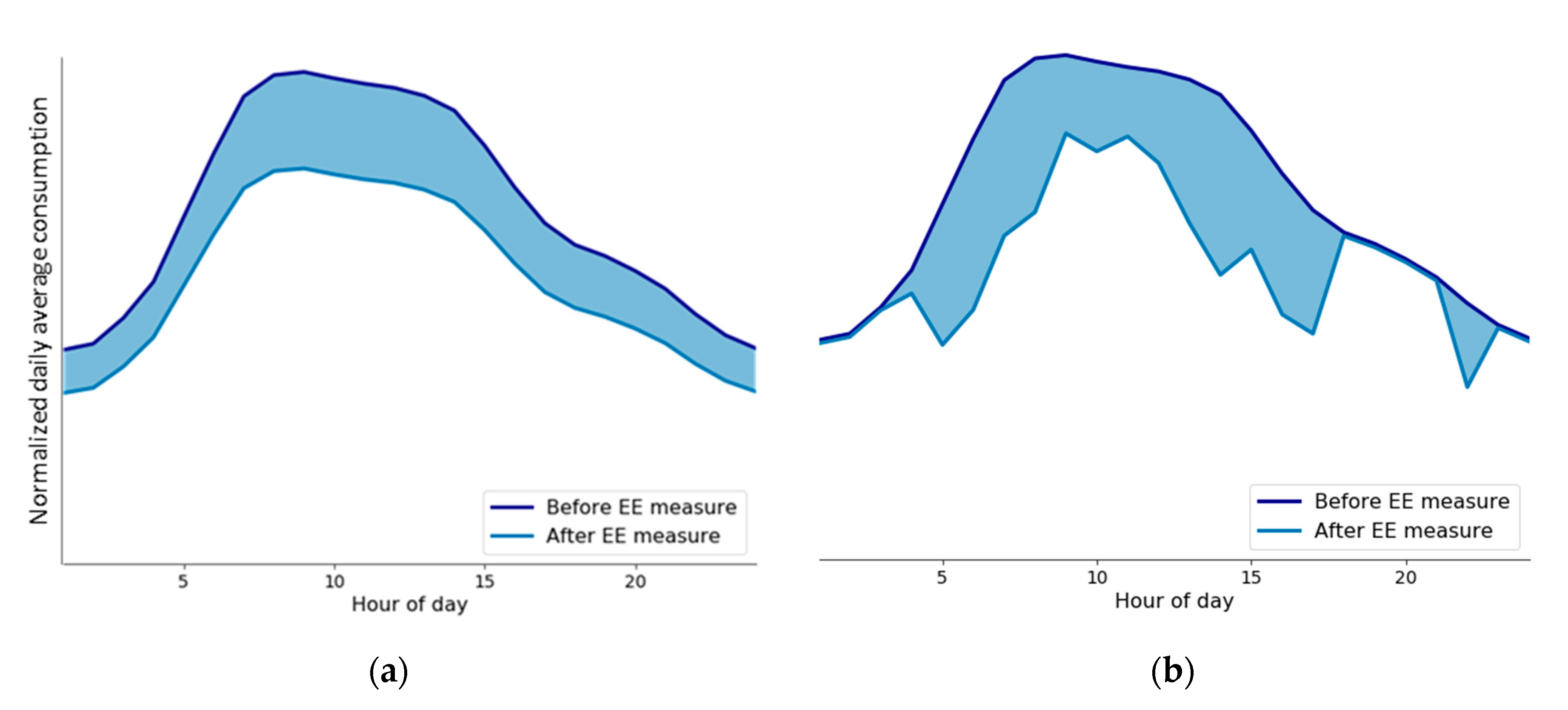Hourly load may increase when recovering from setbacks to the desired temperature in the occupancy period, as opposed to operation at a constant setpoint [28].

define the example of residential and commercial measures in terms of the targeted end-use, baseline load shape and operation, level of electricity demand post-measure, and control technology. All measures assume a fairly inefficient technology and operation baseline (e.g., single-stage compressors, fluorescent lighting, manual control). The savings shape of each measure is driven by the difference between the more efficient technology and this inefficient baseline. To derive directional EE and DR interactions in the framework (i.e., complement versus compete), we first characterize the passive load shape (“post EE load shape”) as being in one of two possible states. First, the load shape following the EE investment may represent an overall percent reduction, maintaining a similar shape. For example, commercial lighting EE measures based on more efficient lamps or fixtures tend to have hourly impacts proportional to the underlying lighting end-use hourly shape (see Figure 1, panel a). We describe this passive load shape as “generally lower” (i.e., lower energy consumption in most/all hours of the year). Second, the passive load shape may look quite different on an hourly or sub-hourly basis when an EE or DR investment includes controls technology, thermal improvements, or different operational strategies. For example, commercial lighting occupancy sensors may produce hourly impacts asynchronous to the baseline lighting end-use hourly shape as the sensors function based on the timing of human presence in specific locations and not the pre-existing lighting schedule (see Figure 1, panel b) [25]. We describe this passive load shape as “sometimes lower and sometimes higher” (i.e., lower energy consumption in some hours of the year and potentially higher energy consumption in other hours of the year).

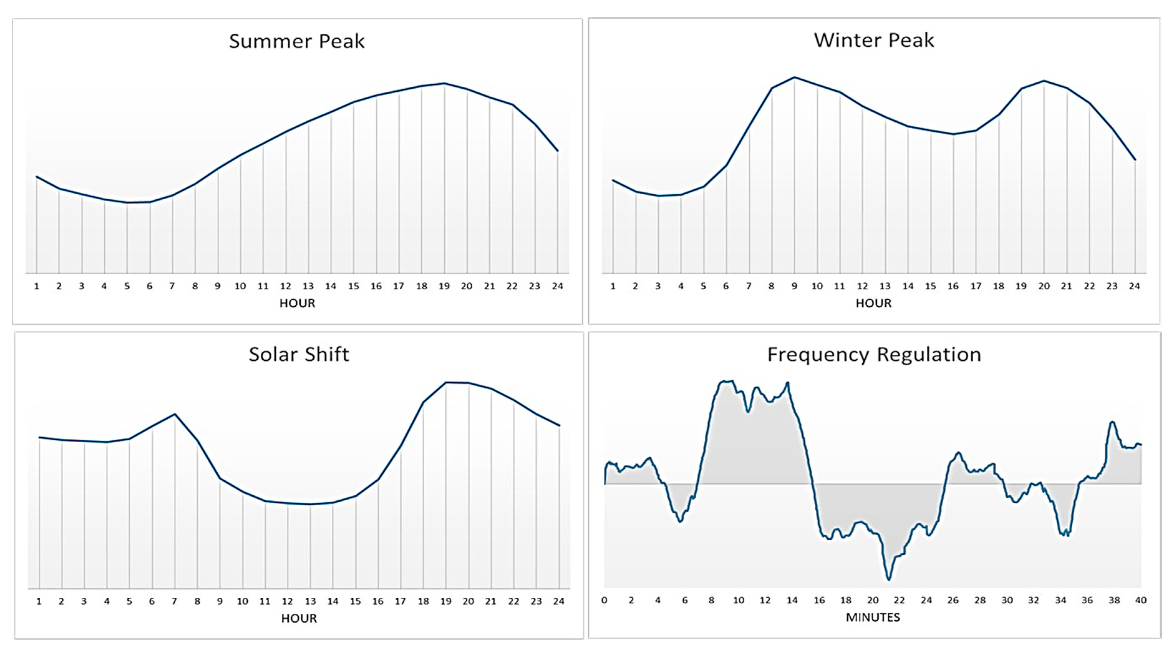
The second level of our framework can only be defined in relation to specific system conditions that can change at intervals ranging from seconds to hours based on several factors (e.g., load, generating resource, voltage, frequency, and transmission congestion). As such, we develop a limited number of utility system prototypes intended to generalize the system conditions that we consider the most significant for EE and DR interactions (see Figure 2). These system prototypes are then considered when applying Levels 2a and 2b of the framework. The system prototypes are defined as follows:

• Summer peak shed: system need to reduce summer peak demand (i.e., shed) driven by high temperatures and AC load.
• Winter peak shed: system need to reduce winter peak demand (i.e., shed) driven by low temperatures and heating load.
• Solar shift: system need to shift load from high to low photovoltaic production periods to avoid renewable energy curtailment driven by high solar generation.
• Frequency reserves: system need to provide frequency reserves (i.e., modulate).

3. Results

In the following sections, we qualitatively assess each level of our framework in detail, using these specific EE measures and system prototypes, to highlight important issues that can arise in applying the framework in specific contexts.

3.1. Level 1a-Change in Building Demand Flexibility

This first sublevel of the framework is focused on the change in the building-level DF due to an EE or DR investment. Whether EE and DR compete with or complement each other at Level 1a is a function of two distinct changes to DF: (1) the change in technical potential, as defined by the change in passive load shape, reflects whether and how the underlying load shape changes following an EE or DR investment (e.g., if the load is lower in all hours, there is less load technically available to participate in DR programs); and (2) the change in capability reflects whether and how the building is more or less able to reliably provide a responsive or flexible resource when needed by the utility. The concept of reliability is represented here by automation or remote controllability that increases DF without changing anything about how much load can be controlled. We group our measures by the change in passive load shape and the change in capability to provide demand flexibility, which are the two components of Level 1a (see

Table 4. Examples of change in passive load shape and change in capability for a building to provide demand flexibility (Level 1a).

			Change in Passive Load Shape
			Generally lower	Sometimes lower/sometimes higher
Change in capability	Unchanged	Without controls	Res. ERWH wrap Res. HPWH Com. LED lighting Com. refrigeration upgrade Com. variable speed AC	No examples considered
	Higher	Without controls	No examples considered	Com. building envelope upgrade
		With controls	Res. ERWH wrap + grid connection Com. refrigeration upgrade + controls	Res. PCT Res. grid connected HPWH Com. networked lighting controls Com. variable speed AC + PCT

).

The measures in the top row (i.e., Res. electric resistance water heater (ERWH) wrap, Res. heat pump water heater (HPWH), Com. LED lighting, Com. refrigeration upgrade, and Com. variable speed AC) have lower demand in all hours of operation (driving a reduction in DF technical potential) and do not include control technologies (resulting in no change in capability), as compared to the baseline load profile and capabilities prior to the EE or DR investment. Essentially, among these measures there is less load to provide as a flexible resource and no increased ability to reduce the load, shift it into different time periods, or respond at sub-hourly timescales for modulation. Therefore at Level 1a for these measures, EE and DR compete with each other for load shed, shift, and modulation.

The second row contains only one measure—commercial building envelope upgrade—with a passive state demand that is sometimes lower and sometimes higher. If heating, ventilation, and air conditioning (HVAC) operations are unchanged, demand is generally lower during peak daytime cooling hours, due to reduced thermal losses through the building shell, but may be increased (though still small relative to peak loads) during the overnight hours, since passive cooling is less effective and more mechanical cooling is required. The change in the passive load shape, therefore, either increases or decreases technical potential depending on the specific hour under consideration. In addition, the building may now also be able to more effectively employ pre-heating or pre-cooling strategies that shift the timing of the consumption in response to time-varying electricity rates (utilizing the existing thermostat or other HVAC controls). More specifically, efficient commercial building envelopes would likely increase the building’s ability to maintain indoor temperatures without increasing demand during the peak period but not necessarily increase the ability to increase demand during the pre-cooling or pre-heating hours, which would also be limited by service-level thresholds (e.g., over-cooling occupants in the middle of a summer day).

While not a result of new control technologies associated with the measure, the enhanced effectiveness of pre-heating or pre-cooling increases the DF capability specifically for load shifting. Similarly, the improved thermal stability of the building may allow cooling loads to be shed for a longer duration without unacceptably degrading occupant comfort. Thus, for this measure, EE and DR may either compete with or complement each other at Level 1a, depending on the particular timing of the system need and on whether the increased DF capability from improved thermal stability outweighs the reduction in the DF technical potential (total available load) during peak hours.

The final row of measures in Table 4 adds controls to the change in passive state demand. Residential ERWH wrap + grid connection and commercial refrigeration upgrade + controls have a lower load in all hours after the EE investment and, in our examples, include the addition of programmable controls. Similarly, the remaining examples (i.e., Res. PCT, Res. grid-connected HPWH, Com. variable speed AC, and Com. networked lighting controls) combine the addition of controls with a post-measure load shape that is sometimes lower and sometimes higher. Whether EE and DR compete with or complement each other in these cases depends on whether the reduced technical potential has a greater or smaller impact than the additional capability to control loads. Prior studies suggest the addition of capability via controls may overcome the reduced technical potential, thus driving complementary interactions between EE and DR [32,33].

3.2. Level 1b-Change in the Fraction of Building Demand Flexibility Participating as a Demand Response Resource

The second sublevel of the framework is focused on the change in the fraction of the building’s DF (computed relative to the total DF following any changes at Level 1a) that participates as a DR resource. Changes at Level 1b are considered from the perspective of the participating customer. They do not encompass changes in technical potential and capability, which are addressed at Level 1a, but rather they encompass changes that may occur in participation drivers, like changes in customer comfort and financial incentives. In other words, Level 1a is about the change in technical potential and capability, and Level 1b is about how much of the technical potential and capability is participating and being utilized. Therefore, to fully assess whether EE and DR compete with or complement each other with respect to the fraction of DF that is participating, Level 1b must take into account participant preferences, behavior, and programmatic factors (e.g., methodologies for computing customer baselines, retail rate design, financial incentive payments, and/or customer override capabilities).

The example measures point to three key factors driving EE and DR interactions at Level 1b: (1) customer participation prior to the measurement of installation; (2) change in customer baseline and resultant impacts on financial incentives for participation; and (3) additional controls or new capabilities to alter the timing of consumption.

First, it matters whether the customer is able to participate in DR prior to the measure. For example, consider a residential electric resistance water heater. Without utility dispatch (e.g., a utility direct load control switch) or customer programmable controls (e.g., a programmable thermostat), the water heater is difficult to turn off manually, thereby precluding event response. Simply improving the efficiency of this end-use, whether through improved tank insulation or replacement with an HPWH, would not be expected to change the fraction of the DF participating as a DR resource. Similarly, commercial refrigeration cannot easily be manually controlled to provide a DR resource. Commercial refrigeration may also need to meet local, state, or federal guidelines or regulations for food safety, thereby prohibiting participation.

Second, measures that result in a new, lower customer baseline would reduce DR participation payments thereby eroding financial incentives to participate. In the commercial building envelope upgrade example, we assume the building’s capability to shed or shift load has increased since its thermal retention properties have improved, enabling greater reduction in space conditioning without disrupting building services. However, the building’s passive load shape is also lower during peak hours, and the customer may be less willing to participate if the DR financial incentive is reduced because the building has a smaller baseline load. It is also worth noting that competition between EE and DR may occur in situations where the EE investment precludes the customer from participating as a DR resource, as is the case for some residential water heater DR programs that do not include HPWH as an eligible end-use [34].

Third, measures that increase DF capability, either via operational strategies or controls, are likely to increase the fraction of DF participating as a DR resource. For example, smart thermostat control capability (represented in the Res. PCT example) allows load reductions to be achieved regardless of occupancy (i.e., the thermostat can be adjusted automatically or remotely) and with less concern that the result will be unacceptable to the occupants, increasing the fraction of DF participation in individual DR events. Commercial lighting controls capability (represented in the Com. networked lighting controls example) allows load reductions to be achieved with a more uniform lighting density (in comparison to switching off banks of luminaires, for example) and again with minimal occupancy impact. Because lighting levels can be controlled in ways that have minimal or no disruption to operation, the fraction of DF participating in DR is likely greater than that of the pre-measure state.

3.3. Level 2a-Change in Utility System Need for DR

The third sublevel of the framework is focused on the change in the need for DR resources in the utility system. Unlike Levels 1a (change in building DF) and 1b (change in building DF participation fraction), which take the building perspective, Levels 2a and 2b of the framework take the utility system perspective. Levels 2a and 2b also differ from Levels 1a and 1b by considering DR instead of DF. As discussed in Section 2.1, the framework distinguishes DR as the system resource and DF as the potential or opportunity. Levels 2a and 2b are, therefore, concerned with the change in system resources. Levels 2a and 2b first account for the impacts of EE on utility system loads and resources and then consider the change in the utility system need for and availability of DR.

Level 2a specifically considers whether the EE investments made by many customers or building owners have, in aggregate, increased or decreased the likelihood of needing DR resources to address utility system conditions. At this level of the framework, an increase in system need reflects competition, whereas a decrease in system need reflects complementarity, between EE and DR. Interactions between EE and DR at Level 2a are almost entirely driven by the coincidence of the energy/demand savings at the building level and the net load driving system conditions. The presence of control capabilities is also an important driver, as they may increase or decrease the coincidence of energy/demand savings with system load. This depends on the specifics of how building controls are implemented.

At this level, it is necessary to assess EE and DR interactions in the context of system conditions. Among our summer and winter peak system conditions prototypes, most or all EE measures have a complementary interaction between EE and DR. This is because the reduced load from the EE or DR investment coincides (to some degree) with the utility summer or winter peak. Because the demand savings from the EE investment reduce the summer and winter peaks, there is a reduced need for DR resources (i.e., lower likelihood of reliability or economic system conditions necessitating DR). The degree of complementarity varies depending on the specific example being considered, where end-uses that tend to drive system peaks have much greater complementarity (e.g., AC driving summer peaks, residential ERWH driving winter morning and evening peaks) than end-uses that are less coincident with system peaks (e.g., commercial refrigeration that operates over many hours of the day).

Among the example measures, EE and DR more often compete with each other at Level 2a in solar shift and frequency reserve system conditions. The solar shift system condition is characterized by a need to build load during periods when solar generation is greatest yet load is relatively low (typically in the early afternoon periods and during the spring season). Therefore, demand savings in the load building periods (e.g., through more efficient commercial air conditioning) will only exacerbate the potential for renewable energy curtailment and declining net loads. The frequency reserve system condition is, in our example, characterized by the need to quickly increase or decrease generation over short timescales to meet steeply increasing or decreasing generation due to high solar generation penetrations. As generating resources must quickly respond to meet changing load, the timing of some demand savings may increase the steepness of the ramp periods and contribute to the additional need for frequency regulation resources. Of course, these conclusions depend critically on the alignment between demand savings and solar production profiles (e.g., the greater the alignment, the greater the increase in the need for DR), and the degree of competition may vary throughout the year.

3.4. Level 2b Change in the Availability of DR

The fourth sublevel of the framework is focused on the change in the availability of DR in the utility system. Dispatchable resources like DR are used by utility system operators to meet system conditions and need to maintain electricity reliability and service levels. EE may interact with DR by increasing or decreasing the amount of DR that is available to utility system operators. Whether EE and DR compete with or complement each other at Level 2b of our framework depends largely on the net effect of Levels 1a (change in building DF) and 1b (change in building DF participation fraction). Specifically, this depends on the interplay between the change in passive load shape, the addition of capabilities (e.g., via controls or operational strategies), and change in participation.

The primary driver of the interaction between EE and DR at Level 2b is the aggregate amount of demand flexibility available during times of system need that can be converted into a system resource. Electrical end-uses in commercial buildings have load shapes (post-EE) that closely match solar generation production curves, and EE measures likely have their greatest impact when the load is high. Therefore, while a building could increase consumption by pre-cooling in hours of high solar production during the day, there is limited load available to shed during the evening and nighttime hours due to the operation hours of commercial buildings. As such, there is a smaller load to displace or “shift” from the evening ramp and nighttime hours. Certain operational or technical characteristics of some end-uses also limit their availability as a DR resource. For example, commercial lighting cannot be stored or readily rescheduled and thus is not a load that can be shifted on demand. Similarly, heating or cooling loads do not typically occur outside their respective seasons (i.e., heating demand occurs in colder seasons and cooling demand occurs in warmer seasons).

EE and DR complementarity at Level 2b is most likely to occur with the addition of controls and operational strategies that increase both the resource capabilities (Level 1a change in building DF for an individual building) and participation (Level 1b change in building DF participation fraction). For example, smart thermostats (and other control technologies) enable a more flexible and reliable DR resource, providing the system operator more DR to dispatch when needed. Additionally, an improved commercial building envelope can maintain comfort with reduced cooling for longer periods and can pre-cool more effectively, increasing the ability for DR resources to reduce consumption or to shift from peak to off-peak periods.

4. Discussion

Among our measures, we identify three key attributes qualitatively driving EE and DR interactions. First, the change in the passive load shape is an important determinant of whether EE and DR compete with or complement each other. Some of our example measures have post-EE measure load shapes that are lower in all hours of the day, while there are other examples with post-EE demand that is sometimes lower and sometimes higher. Any reduction in the post-EE measure load shape would reduce the total level of load, which would reduce the amount of DF, all else being equal. In such cases, EE and DR compete with each other at Level 1a (change in building DF) because there is less load available to participate in DR (as in the Res. ERWH wrap example). Furthermore, in these cases, EE and DR complement each other at Level 2a (change in utility system need for DR) for load shedding system events because system peak loads are reduced. In contrast, if the post-EE load shape is higher in some hours, this would increase the amount of DF in those hours, all else being equal. In such cases, EE and DR complement each other at Level 1a (at least in some hours) because there is more load available to participate in DR. However, if these hours correspond to the system peak, EE and DR compete with each other at Level 2a for load shedding system events because system peak loads are now higher.

Second, some EE measures increase the DR capabilities of the affected load, via either the addition of controls or operational strategies to shift load. Despite reductions in the post-EE measure load shape, affected loads with increased capabilities to modify load enable access to previously untapped DF. Increased capability may occur via the addition of controls technologies that allow for pre-programmed DR strategies with varying degrees of human-intervention [35] or via the implementation of operational strategies that change the timing of electricity consumption to improve end-use efficiency and DR performance [36]. In addition, some control technologies allow for direct utility dispatch of end-uses (e.g., residential AC compressor cycling). If the increase in capabilities exceeds the concurrent decrease in the load shape, then this tends to suggest more complementarity between EE and DR, particularly at Levels 1a (change in building DF) and 2b (change in DR availability) of the framework. With the incremental addition of controls and utility communication/dispatch, several measures could provide modulation (driving complementarity at Level 2b). Controls and utility communication/dispatch also likely increase the fraction of DF participating in shed and shift events, by increasing the reliability of the response, thus driving complementarity at Level 1b (change in building DF participation fraction). Ultimately, whether or not EE and DR complement each other with additional capability from a load–impacts standpoint depends on the extent of the change in passive load shape (which reduces the overall DR resource) compared with the offsetting increase in load flexibility, fraction of DF participating, and reliability of the DF.

Third, we found that the timing of savings and whether they are coincident with peak or load–building periods mattered at Levels 2a (change in utility system need for DR) and 2b (change in DR availability). Importantly, we find few examples among our commercial measures that reduce the system need for load shifting in the “solar shift” system condition due to the fact that savings tend to occur in the times when the system needs to increase load. It is important, therefore, to consider the temporal dimension of EE and DR relative to the system shape as this defines much of their value to the utility system. This is especially significant for grid systems with a high amount of VRE generation that can dramatically and unpredictably alter hourly or sub-hourly marginal costs. Utilities should, therefore, employ strategies to maximize the overall reduction in energy consumption from EE measures, while avoiding competitive effects between EE and DR arising from the timing of load reductions.

5. Conclusions

We developed and described a conceptual framework that characterizes the ways in which EE and DR compete with and complement each other at the individual building and aggregate system level. We used example measures to qualitatively show the application of the framework and highlight key drivers of complementarity and competition.

Importantly, we find no universal relationship between EE and DR. Instead we find that EE and DR interactions depend on measure and technology specifics (including building type and targeted end-use), as well as utility system conditions. We also find that EE and DR interactions are defined by more than just the change in discretionary load (i.e., DR potential) but also the change in the likelihood of participation in DR programs, as well as the change in system need for, and the overall availability of, DR resources. This high-level framework can encourage regulators and utilities to co-optimize EE and DR program design and funding in order to more efficiently deploy and use DERs.

The flexibility of this framework allows it to work under various scenarios and be applied to research on integrated building systems in several ways. First, analysis quantifying EE and DR resource potential may benefit from grouping measures into portfolios with different likely implications for EE and DR interactions. For example, equipment upgrades involve the installation of more efficient appliances, equipment, electronics, or lighting products. These will tend to reduce the amount of flexible load at the building level, but they may also reduce the grid need for DR. Additionally, controls measures involve the installation of control technologies (e.g., programmable thermostats or occupancy sensors) that can reduce overall energy consumption. These will tend to increase DF at the building level, but, depending on the control strategies used, they may either increase or decrease the need for DR at the utility system levels. Last, envelope improvements will tend to increase DF at the building level because space conditioning loads can be reduced for a longer period of time without affecting occupant comfort. Building envelope improvements may also reduce the need for DR at the system level by decreasing peak loads.

Our qualitative application of the framework to a subset of EE and DR measures suggests increasing complexity in evaluating EE and DR interactions when moving from standalone equipment to integrated systems. The EE and DR capabilities of standalone equipment are generally easy to evaluate at a component level with minimal interaction with the rest of the building. Examples of standalone equipment that has minimal influence on the rest of the building include ERWH, HPWH, appliances, plug loads and miscellaneous equipment loads, elevators, and pool pumps. Building-integrated systems such as HVAC and lighting systems, by contrast, are integrated with the building structure. HVAC loads are related to the building façade, windows, walls, and building mass. Lighting needs are also related to windows, and passive daylight may be available in many building configurations. While integrated systems may have more difficult-to-quantify EE and DR interactions, they may also be the most significant in terms of accessing DF through the addition of DR capabilities (e.g., EE retrofits that influence the façade will influence the need for DR and the DR capabilities of HVAC and lighting systems). In addition, many integrated systems that can drive increased DF participation in DR programs will also enhance customer comfort (e.g., HVAC and lighting controls provide visual and thermal comfort and air quality). The framework can inform the design of EE and DR programs that incorporate complementarity to bring down enablement and incentive costs and achieve higher energy savings and emissions reductions as part of integrated building system designs.