Performance Comparison between Two Established Microgrid Planning MILP Methodologies Tested On 13 Microgrid Projects


Abstract
:1. Introduction
2. Model Description and Used Data Down-Sampling
2.1. Peak Preserving Day-Types Representative Optimization (RO)
RO MILP
| Indices | |
| continuous generation technologies (assumed to be available in any size), = {photovoltaic panels, solar thermal panels, and absorption chillers} | |
| day-types, = {week, peak, weekend} | |
| discrete generation technologies (explicitly modeled in discrete sizes), internal combustion engines (ICE), micro turbines (MT), fuel cells (FC), and gas turbines (GT), with and without heat exchangers (HX), = {ICE, ICEHX, MT, MTHX, FC, FCHX, GT, GTHX}. All discrete technologies without HX are referred to as DG, DG with HX as CHP | |
| hours in a day | |
| DER technologies, | |
| generation technologies, | |
| months in a year, | |
| utility demand periods, = {coincident, on peak, mid peak, off peak} | |
| energy storage technologies, stationary storage and heat storage, = {electric energy storage systems, heat storage} | |
| energy end-uses for each day-type (d), including electricity-only (eo), cooling (cl), space heating (sh), water heating (wh), and natural gas loads (ng), = {eo, cl, sh, wh, ng} | |
| Parameters | |
| annuity rate of investing in DER technology i | |
| NDm,d | number of days of type d in month m |
| volumetric electricity charges | |
| charges applied to peak power demand for end-use u during period p, and month m | |
| volumetric demand response costs | |
| fuel costs, maintenance costs | |
| fixed investment cost of DER technology i | |
| variable investment cost of continuous energy conversion technology c, or storage technology s | |
| Microgrid energy demand for end-use u, in month m, day-type d, and hour h | |
| fixed monthly utility charges/contract demand charges | |
| electricity sales price in month m, day-type d, and hour h | |
| ηi | energy conversion efficiency for i |
| Decision Variables | |
| installed capacity of continuous generation technology c, or storage technology s | |
| energy demand of end-use u removed by demand response measures in month m, day d, and hour h | |
| useful (e.g., electric output) energy provided by generation technology j for end-use u in month m, day-type d, and hour h | |
| number of installed units of discrete generation technology g | |
| binary purchase decision for continuous generation technology c, or storage technology s | |
| energy sales from technology i that is exported in month m, day-type d, and hour h | |
| energy input to storage technology s, in month m, day-type d, and hour h | |
| energy output from storage technology s for end-use u, in month m, day-type d, and hour h | |
| utility purchase for end-use u, during month m, day-type d, and hour h | |
2.2. Full-Scale Time-Series Optimization (FSO)
3. Microgrid Projects
3.1. General Description of Microgrid Projects
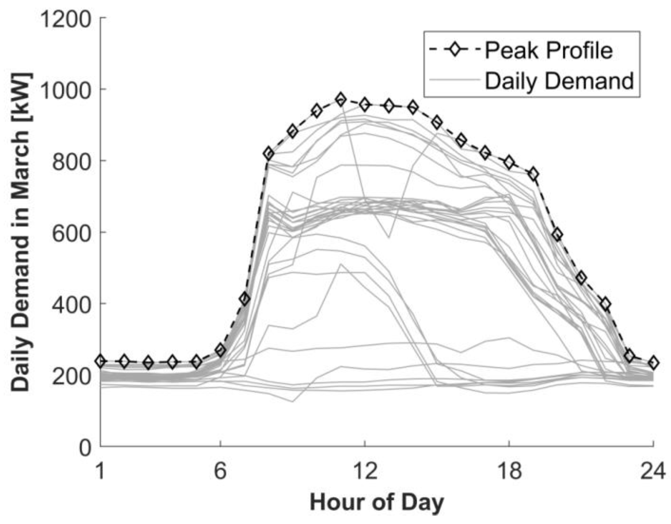
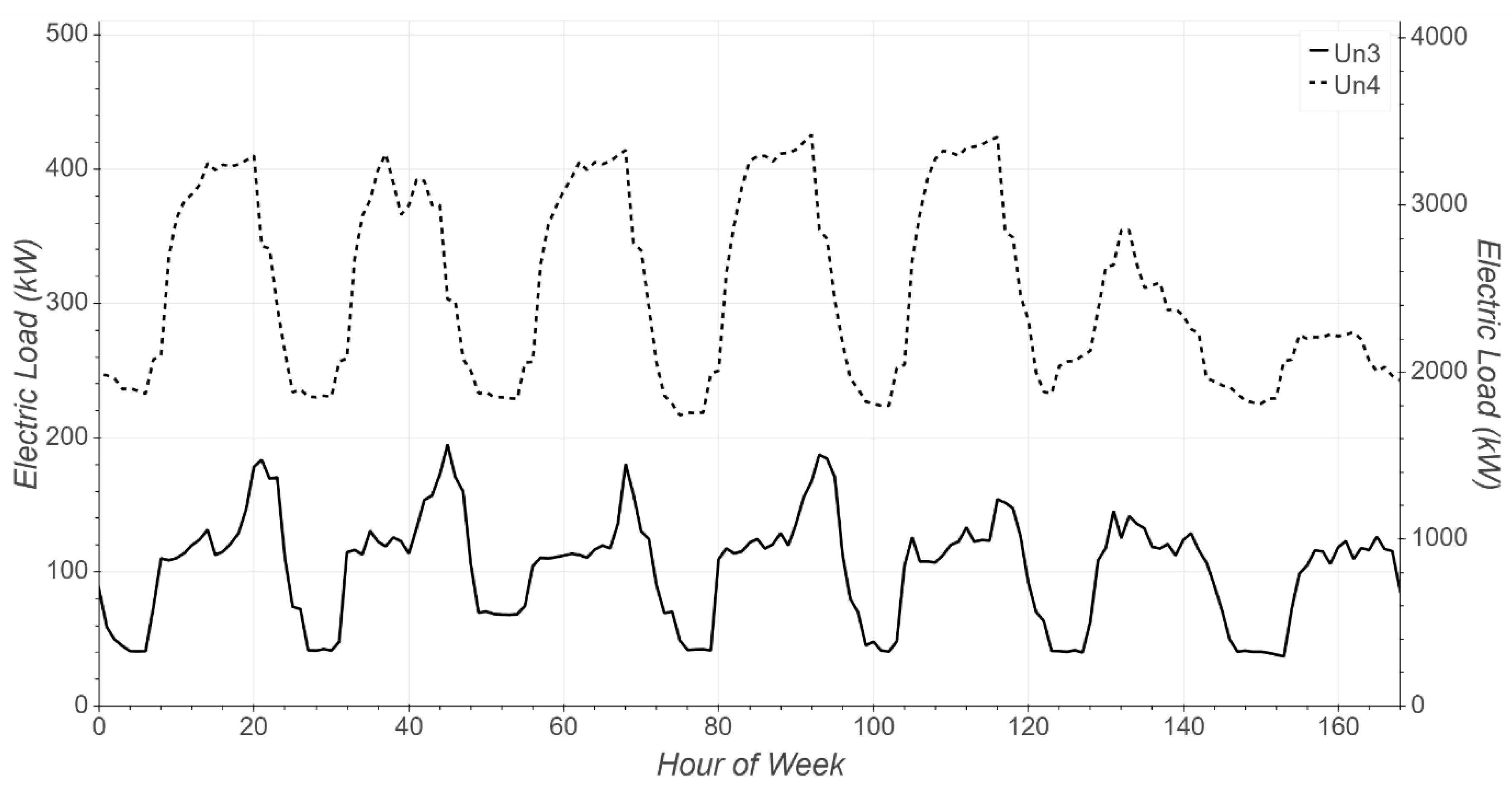
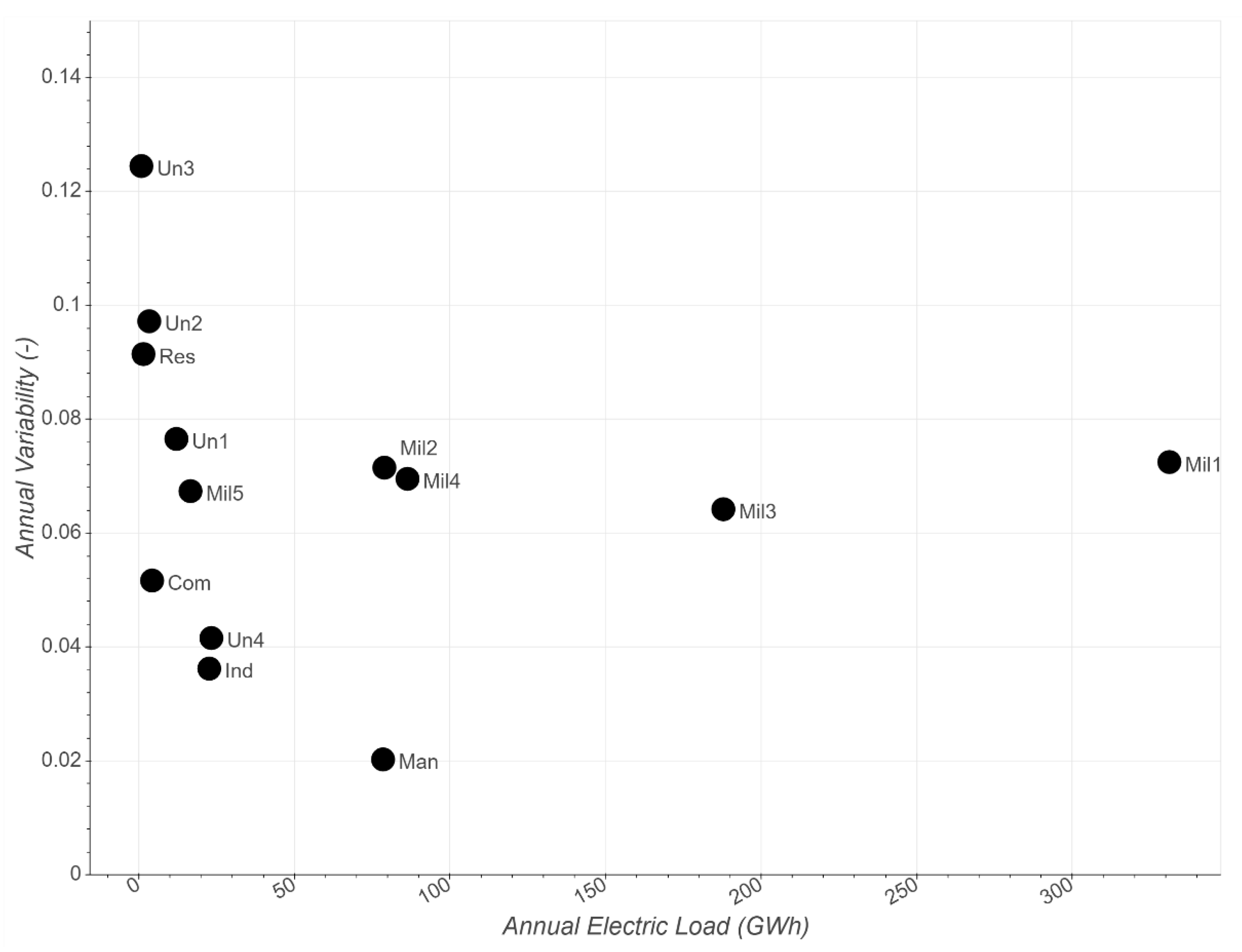
3.2. Electric Load Data
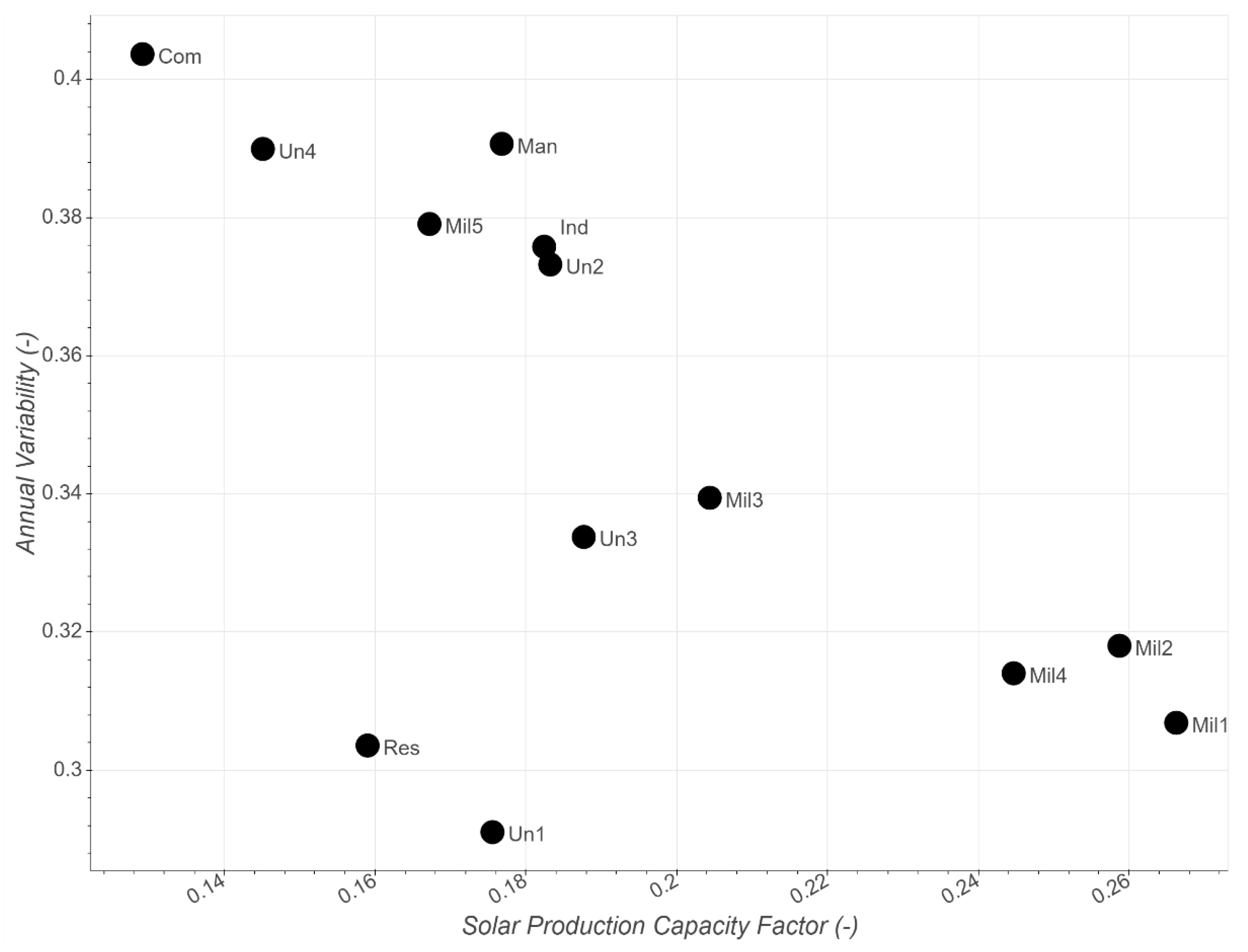
3.3. Solar Radiation Data
4. Results
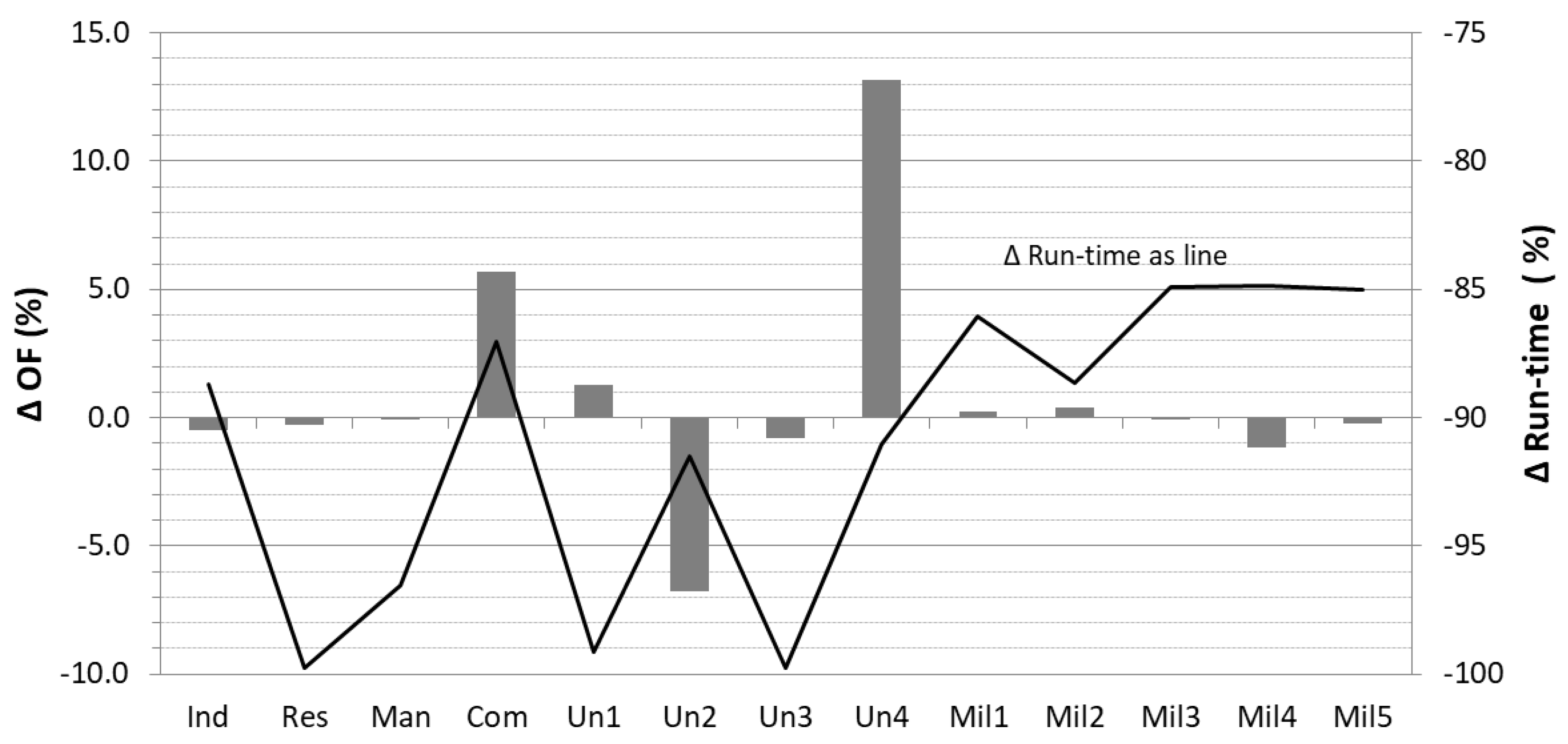
4.1. Representative Optimization (RO) versus Full-Scale Time-Series Optimization (FSO)
4.2. Sensitivity to Electricity Sales
4.3. The Influence of Optimal Dispatch Modeling—The Hybrid Optimization (HO)
5. Conclusions
Author Contributions
Funding
Acknowledgments
Conflicts of Interest
Appendix A. Tariff Data

| Tariff Data | |||||
|---|---|---|---|---|---|
| Case | Type | State | Utility Name | Tariff Name | Source Document |
| Ind | Industrial/Pharmaceutical | Puerto Rico | Puerto Rico Electric Power Authority (PREPA) | LIS | [28] |
| Res | Residential/Public | Connecticut | Eversource Energy | Rate 56—Intermediate Time of Day | [29] |
| Man | Industrial/Materials | Puerto Rico | PREPA | GST | [28] |
| Com | Commercial/Public | Washington State | Seattle City Light | MDC—Medium General Service: city | [30] |
| Un1 | University | Colorado | Black Hills Energy | CO935—LPS-PTOU | [31] |
| Un2 | University | Hawai’i | HECO | HECO-P | [32] |
| Un3 | University | California | SDGE | AL-TOU | [33] |
| Un4 | University | Vermont | CBE | Rate 08—General Service | [34] |
| Mil1 | Military | Texas | Confidential | Confidential | Confidential |
| Mil2 | Military | New Mexico | Confidential | Confidential | Confidential |
| Mil3 | Military | Maryland | Confidential | Large Power Schedule | Confidential |
| Mil4 | Military | California | Confidential | Confidential | Confidential |
| Mil5 | Military | Massachusetts | Confidential | Industrial Service | Confidential |
Appendix B. Technology Data
| Case | PV Technology Assumptions | ||||||
|---|---|---|---|---|---|---|---|
| PV Costs ($/kWDC) | O&M Costs ($/kW and Month) | Lifetime (yrs.) | Electric Efficiency (%) | Tilt (Degrees/Confidential) | Orientation (South/North, West, East, Confidential) | Max. Space for PV (m2) | |
| Ind | 2150 | 0 | 30 | 16% | 20 | South | 10,000 |
| Res | 2100 | 2.2 | 30 | 19% | Confidential | Confidential | 3760 |
| Man | 2100 | 1.4 | 30 | 16% | 17 | South | 31,876 |
| Com | 1470 | 0 | 30 | 16% | 35 | South | Unrestricted |
| Un1 | 1969 | 0.8 | 25 | 19% | Confidential | Confidential | Unrestricted |
| Un2 | 5000 | 0.8 | 25 | 15% | 22 | South east | 20,000 |
| Un3 | 1700 | 1.4 | 30 | 16% | Confidential | Confidential | 40,000 |
| Un4 | 2400 | 0 | 30 | 19% | 30 | South | 41,806 |
| Mil1 | 1470 | 1.5 | 20 | 15% | Confidential | Confidential | Unrestricted |
| Mil2 | 1470 | 1.5 | 20 | 15% | Confidential | Confidential | Unrestricted |
| Mil3 | 1700 | 1.4 | 20 | 15% | Confidential | Confidential | Unrestricted |
| Mil4 | 1700 | 1.4 | 20 | 15% | Confidential | Confidential | Unrestricted |
| Mil5 | 1700 | 1.4 | 20 | 15% | Confidential | Confidential | Unrestricted |
| Case | EES Technology Assumptions | |||||||||
|---|---|---|---|---|---|---|---|---|---|---|
| Effective EES Costs ($/kWh) | O&M Cost ($/kW Month) | Lifetime (yrs.) | Charging/Respectively Discharge Efficiency (%) | Max. Allowed Charge Rate (-) | Max. Allowed Discharge Rate (-) | Min. SOC (-) | Max. SOC (-) | Maximum Allowed Cycles Per Year (-) | Self-Discharge Per Hour (-) | |
| Ind | 250 | 0 | 5 | 90% | 0.3 | 0.3 | 0.3 | 1 | n/a | 0.001 |
| Res | 350 | 0 | 15 | 90% | 0.3 | 1 | 0.1 | 1 | n/a | 0.0001 |
| Man | 500 | 0 | 20 | 94% | 0.2 | 0.2 | 0.1 | 1 | n/a | 0 |
| Com | 350 | 0 | 20 | 94% | 0.2 | 0.2 | 0.1 | 1 | n/a | 0.001 |
| Un1 | 675 | 0.2 | 25 | 92% | 0.3 | 0.3 | 0.1 | 1 | 110 | 0 |
| Un2 | 566 | 0.2 | 25 | 90% | 0.3 | 0.3 | 0.1 | 1 | n/a | 0.0001 |
| Un3 | 500 | 0 | 20 | 94% | 0.2 | 0.2 | 0.1 | 1 | n/a | 0 |
| Un4 | 350 | 0 | 20 | 90% | 0.5 | 0.3 | 0.1 | 1 | n/a | 0.0001 |
| Mil1 | 212 | 0.3 | 18 | 87% | 0.3 | 0.3 | 0 | 1 | n/a | 0.01 |
| Mil2 | 212 | 0.3 | 18 | 87% | 0.3 | 0.3 | 0 | 1 | n/a | 0.01 |
| Mil3 | 212 | 0.3 | 18 | 87% | 0.3 | 0.3 | 0 | 1 | n/a | 0.01 |
| Mil4 | 212 | 0.3 | 18 | 87% | 0.3 | 0.3 | 0 | 1 | n/a | 0.01 |
| Mil5 | 212 | 0.3 | 18 | 87% | 0.3 | 0.3 | 0 | 1 | n/a | 0.01 |
| DG/CHP Assumptions | ||||||||||
|---|---|---|---|---|---|---|---|---|---|---|
| Case | Type (/) | Unit Capacity (kW) | Lifetime (yrs.) | Capacity Costs Installed ($/kW) | O&M Fixed Costs ($/kW/year) | O&M Variable Cost ($/kWh) | Efficiency (%) | Heat to Power Ratio (%) | Max. Annual Operating Hours (hrs.) | Backup Only (Yes/No) |
| Ind | n/a | n/a | n/a | n/a | n/a | n/a | n/a | n/a | n/a | n/a |
| Res | Microturbine | 60 | 15 | 3220 | 0.0 | 0.001 | 25% | n/a | 8760 | no |
| Microturbine | 100 | 15 | 3500 | 0.0 | 0.002 | 40% | n/a | 8760 | no | |
| Man | CHP | 3304 | 20 | 3281 | 0.0 | 0.009 | 24% | 175% | 8760 | no |
| CHP | 3325 | 20 | 3750 | 0.0 | 0.009 | 44% | 94% | 8760 | no | |
| CHP | 5670 | 20 | 3750 | 0.0 | 0.009 | 28% | 135% | 8760 | no | |
| CHP | 7480 | 20 | 3705 | 0.0 | 0.009 | 45% | 33% | 8760 | no | |
| Com | Microturbine CHP | 61 | 15 | 3220 | 0.0 | 0.013 | 25% | 189% | 8760 | no |
| Microturbine CHP | 190 | 15 | 3150 | 0.0 | 0.016 | 28% | 133% | 8760 | no | |
| Microturbine CHP | 242 | 15 | 2700 | 0.0 | 0.012 | 26% | 145% | 8760 | no | |
| Microturbine CHP | 950 | 15 | 2500 | 0.0 | 0.012 | 28% | 130% | 8760 | no | |
| Un1 | Distributed Generation | 250 | 25 | 2191 | 0.0 | 0.022 | 23% | n/a | 160 | no |
| Distributed Generation | 250 | 25 | 2191 | 0.0 | 0.022 | 23% | n/a | 200 | no | |
| Un2 | n/a | n/a | n/a | n/a | n/a | n/a | n/a | n/a | n/a | n/a |
| Un3 | Internal combustion engine | 125 | 30 | 2000 | 0.0 | 0.020 | 26% | n/a | 8760 | no |
| Un4 | Microturbine | 100 | 15 | 2900 | 0.0 | 0.002 | 30% | n/a | 8760 | no |
| Mil1 | Diesel genset | 2000 | 20 | 600 | 10.0 | 0.000 | 32% | n/a | 8760 | yes |
| Mil2 | Diesel genset | 750 | 20 | 750 | 9.3 | 0.000 | 28% | n/a | 8760 | yes |
| Diesel genset | 750 | 20 | 750 | 9.3 | 0.000 | 28% | n/a | 1091 | no | |
| Mil3 | Diesel genset | 750 | 20 | 750 | 9.3 | 0.000 | 28% | n/a | 8760 | yes |
| Mil4 | Diesel genset | 750 | 20 | 750 | 9.3 | 0.000 | 28% | n/a | 8760 | yes |
| Mil5 | Diesel genset | 750 | 20 | 750 | 9.3 | 0.000 | 28% | n/a | 8760 | yes |
References
- Navigant. Microgrid Deployment Tracker 2Q18; Navigant: Chicago, IL, USA, 2018. [Google Scholar]
- Navigant. Microgrid Deployment Tracker 2Q19; Navigant: Chicago, IL, USA, 2019. [Google Scholar]
- Wood, E. Whats Driving Microgrids toward a $30.9B Market? Microgrid Knowledge. 30 August 2018. Available online: https://microgridknowledge.com/microgrid-market-navigant/ (accessed on 4 March 2020).
- Tozzi, P.; Jo, J.H. A comparative analysis of renewable energy simulation tools: Performance simulation model vs. system optimization. Renew. Sustain. Energy Rev. 2017, 80, 390–398. [Google Scholar] [CrossRef]
- Lund, H.; Arler, F.; Alberg Østergaard, P.; Hvelplund, F.; Connolly, D.; Vad Mathiesenm, B.; Karnøe, P. Simulation versus Optimisation: Theoretical Positions in Energy System Modelling. Energies 2017, 10, 840. [Google Scholar] [CrossRef]
- Fescioglu-Unver, N.; Barlas, A.; Yilmaz, D.; Demli, U.O.; Bulgan, A.C.; Karaoglu, E.C.; Atasoy, T.; Ercin, O. Resource management optimization for a smart microgrid. J. Renew. Sustain. Energy 2019, 11, 065501. [Google Scholar] [CrossRef]
- Stadler, M.; Naslé, A. Planning and Implementation of Bankable Microgrids. Electr. J. 2019, 32, 24–29. [Google Scholar] [CrossRef]
- REopt. Available online: https://reopt.nrel.gov/ (accessed on 4 March 2020).
- DER-CAM. Available online: https://building-microgrid.lbl.gov/projects/der-cam/ (accessed on 4 March 2020).
- Gabrielli, P.; Gazzani, M.; Martelli, E.; Mazzotti, M. Optimal design of multi-energy systems with seasonal storage. Appl. Energy 2018, 219, 408–424. [Google Scholar] [CrossRef]
- Schütz, T.; Schraven, M.H.; Fuchs, M.; Remmen, P.; Müller, D. Comparison of clustering algorithms for the selection of typical demand days for energy system synthesis. Renew. Energy 2018, 129, 570–582. [Google Scholar] [CrossRef]
- Marquant, J.F.; Mavromatidis, G.; Evins, R.; Carmeliet, J. Comparing different temporal dimensions representations in distributed energy system design models. Lausanne. Energy Procedia 2017, 122, 907–912. [Google Scholar] [CrossRef]
- Fahy, K.; Stadler, M.; Pecenak, Z.K.; Kleissl, J. Input data reduction for microgrid sizing and energy cost modeling: Representative days and demand charges. Renew. Sustain. Energy 2019, 11, 065301. [Google Scholar] [CrossRef] [Green Version]
- Bahl, B.; Kümpel, A.; Seele, H.; Lampe, M.; Bardow, A. Time-series aggregation for synthesis problems by bounding error in the objective function. Energy 2017, 135, 900–912. [Google Scholar] [CrossRef]
- Pecenak, Z.K.; Stadler, M.; Mathiesen, P.; Fahy, K.; Kleissl, J. Robust Design of Microgrids Using a Hybrid Minimum Investment Optimization. Appl. Energy 2020, 276, 115400. [Google Scholar] [CrossRef]
- Mashayekh, S.; Stadler, M.; Cardoso, G.; Heleno, M. A Mixed Integer Linear Programming Approach for Optimal DER Portfolio, Sizing, and Placement in Multi-Energy Microgrids. Appl. Energy 2017, 167, 154–168. [Google Scholar] [CrossRef] [Green Version]
- Cardoso, G.; Stadler, M.; Mashayekh, S.; Hartvigsson, E. The impact of Ancillary Services in optimal DER investment decisions. Energy 2017, 130, 99–112. [Google Scholar] [CrossRef] [Green Version]
- Milan, C.; Stadler, M.; Cardoso, G.; Mashayekh, S. Modelling of non-linear CHP efficiency curves in distributed energy systems. Appl. Energy 2015, 148, 334–347. [Google Scholar] [CrossRef] [Green Version]
- Stadler, M.; Groissböck, M.; Cardoso, G.; Marnay, C. Optimizing Distributed Energy Resources and Building Retrofits with the Strategic DER-CAModel. Appl. Energy 2014, 132, 557–567. [Google Scholar] [CrossRef] [Green Version]
- Cardoso, G.; Stadler, M.; Bozchalui, M.C.; Sharma, R.; Marnay, C.; Barbosa-Póvoa, A.; Ferrão, P. Optimal investment and scheduling of distributed energy resources with uncertainty in electric vehicle driving schedules. Energy 2014, 64, 17–30. [Google Scholar] [CrossRef]
- Hanna, R.; Disfani, V.R.; Haghi, H.V.; Victor, D.G.; Kleissl, J. Improving estimates for reliability and cost in microgrid investment planning models. J. Renew. Sustain. Energy 2019, 11, 045302. [Google Scholar] [CrossRef]
- Schittekatte, T.; Stadler, M.; Cardoso, G.; Mashayekh, S.; Sankar, N. The impact of short-term stochastic variability in solar irradiance on optimal microgrid design. IEEE Trans. Smart Grid 2018, 9, 1647–1656. [Google Scholar] [CrossRef] [Green Version]
- Pecenak, Z.K.; Stadler, M.; Fahy, K. Efficient Multi-Year Economic Energy Planning in Microgrids. Appl. Energy 2019, 255, 113771. [Google Scholar] [CrossRef]
- XENDEE. Available online: https://xendee.com (accessed on 4 March 2020).
- OpenEI. Available online: https://openei.org/doe-opendata/dataset/commercial-and-residential-hourly-load-profiles-for-all-tmy3-locations-in-the-united-states/ (accessed on 12 February 2020).
- Helioscope. Available online: https://www.helioscope.com/?gclid=EAIaIQobChMI8rXA-52E6AIVT_lRCh0aQwrNEAAYASAAEgJXY_D_BwE/ (accessed on 12 February 2020).
- Dobos, A.P. PVWatts Version 5 Manual; NREL/TP-6A20-62641; National Renewable Energy Laboratory: Golden, CO, USA, September 2014.
- PREPA. Available online: https://aeepr.com/es-pr/QuienesSomos/Ley57/Facturaci%C3%B3n/Tariff%20Book%20-%20Electric%20Service%20Rates%20and%20Riders%20Revised%20by%20Order%2005172019%20Approved%20by%20Order%2005282019.pdf (accessed on 27 January 2020).
- Eversource. Available online: https://www.eversource.com/content/docs/default-source/rates-tariffs/ct-electric/rate-56-ct.pdf?sfvrsn=e941c762_32 (accessed on 22 January 2020).
- Seattle City Light. Electric Rates and Provisions. Available online: https://www.seattle.gov/light/Rates/docs/2020/Schedule%20MDC%20Jan%201%202020.pdf (accessed on 23 January 2020).
- Black Hills Energy. Schedule of Rates, Rules and Regulations for Electric Service. Available online: https://www.blackhillsenergy.com/sites/blackhillsenergy.com/files/coe-rates-tariff_0.pdf (accessed on 22 January 2020).
- Maui Electric. Schedule “P” Large Power Service. Available online: https://www.mauielectric.com/documents/billing_and_payment/rates/hawaii_electric_light_rates/helco_rates_sch_p.pdf (accessed on 23 January 2020).
- SDGE. Schedule AL-TOU. Available online: Sdge.com/sites/default/files/elec_elec-scheds_al-tou.pdf (accessed on 13 January 2020).
- Burlington Electric. Available online: https://www.burlingtonelectric.com/rates-fees#large-general-service-lg (accessed on 13 January 2020).
- Fu, R.; Feldman, D.J.; Margolis, R.M. U.S. Solar Photovoltaic System Cost Benchmark: Q1 2018; NREL/TP-6A20-72399; National Renewable National Laboratory (NREL): Golden, CO, USA, 2018.
- Cole, W.J.; Frazier, A. Cost Projections for Utility-Scale Battery Storage; NREL/TP-6A20-73222; National Renewable National Laboratory (NREL): Golden, CO, USA, 2019.
- EIA. US Energy Information Administration (EIA). Available online: https://www.eia.gov/outlooks/aeo/assumptions/pdf/commercial.pdf (accessed on 11 March 2020).
- Ericson, S.J.; Olis, D.R. A Comparison of Fuel Choice for Backup Generators; National Renewable Energy Laboratory: Golden, CO, USA, 2019.


| Case | Type | State/Territory | Techn. Modeled | Tariff Characteristics | Annual Electrical Cons. (MWh) | Annual Heating Cons. (MWh) | Electric Peak Load (MW) |
|---|---|---|---|---|---|---|---|
| Ind | Industrial/Pharmaceutical | Puerto Rico | PV, EES | FER, NCDC, PDC, MPDC | 22,642 | n/a | 3.96 |
| Res | Residential/Public | Connecticut | PV, EES, DG | TOUER, NCDC | 1640 | n/a | 0.37 |
| Man | Industrial/Materials | Puerto Rico | PV, EES, CHP | FER, NCDC | 78,400 | 41,854 | 12.48 |
| Com | Commercial/Public | Washington State | PV, EES, CHP | FER, NCDC | 4263 | 667 | 0.93 |
| Un1 | University | Colorado | PV, EES, DG | TOUER-summer, FER-winter, PDC | 12,076 | n/a | 2.85 |
| Un2 | University | Hawai’i | PV, EES | FER, NCDC | 3338 | n/a | 0.97 |
| Un3 | University | California | PV, EES, DG | TOUER, NCDC, PDC | 825 | n/a | 0.20 |
| Un4 | University | Vermont | PV, EES, DG | FER, NCDC | 26,713 | 6817 | 5.00 |
| Mil1 | Military | Texas | PV, EES, DG | TOUER, NCDC | 330,648 | n/a | 67.61 |
| Mil2 | Military | New Mexico | PV, EES, DG | TOUER, NCDC | 78,878 | n/a | 15.99 |
| Mil3 | Military | Maryland | PV, EES, DG | FSER, NCDC | 187,645 | n/a | 33.96 |
| Mil4 | Military | California | PV, EES, DG | TOUER, NCDC | 86,349 | n/a | 15.00 |
| Mil5 | Military | Massachusetts | PV, EES, DG | TOUER, NCDC | 16,564 | n/a | 3.41 |
| Case | 1 | 2 | 3 | 4 | 5 | 6 | 7 | 8 | 9 | 10 | 11 | 12 | 13 |
|---|---|---|---|---|---|---|---|---|---|---|---|---|---|
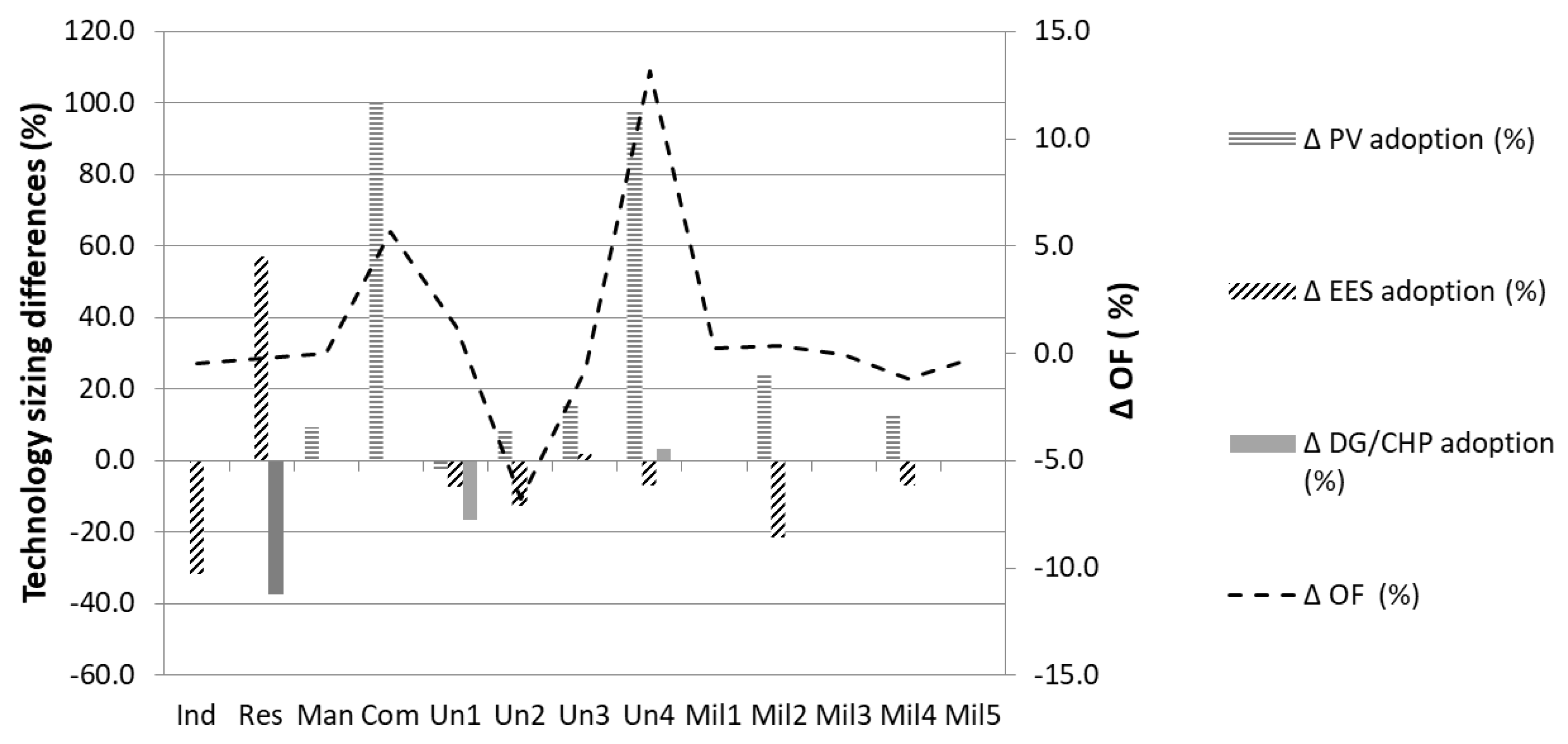
| ∆ OF (%) | R-Time RO (mins) | R-Time FSO (mins) | ∆ R-Time (%) | PV RO (kW) | PV FSO (kW) | ∆ PV Compared to FSO (%) | EES RO (kWh) | EES FSO (kWh) | ∆ EES Compared to FSO (%) | DG/CHP RO (kW) | DG/CHP FSO (kW) | ∆ DG/CHP Compared to FSO (%) | |
| Ind | −0.5 | 0.2 | 1.6 | −89 | 1568 | 1568 | 0.0 | 396 | 582 | −32.0 | 0 | 0 | n/a |
| Res | −0.3 | 0.3 | 121.0 | −100 | 715 | 715 | 0.0 | 1048 | 668 | 56.9 | 100 | 160 | −37.5 |
| Man | 0.0 | 0.3 | 7.4 | −97 | 358 | 328 | 9.1 | 0 | 0 | n/a | 9975 | 9975 | 0 |
| Com | 5.7 | 0.2 | 1.7 | −87 | 182 | 0 | 100.0 *) | 0 | 0 | n/a | 0 | 0 | n/a |
| Un1 | 1.3 | 1.0 | 121.1 | −99 | 8969 | 9211 | −2.6 | 8243 | 8909 | −7.5 | 500 | 600 | −16.7 |
| Un2 | −6.8 | 0.0 | 0.5 | −92 | 1627 | 1501 | 8.4 | 2242 | 2573 | −12.9 | 0 | 0 | n/a |
| Un3 | −0.8 | 0.2 | 88.5 | −100 | 257 | 222 | 15.8 | 320 | 314 | 1.9 | 100 | 100 | 0 |
| Un4 | 13.2 | 0.2 | 2.4 | −91 | 995 | 504 | 97.4 | 2227 | 2400 | −7.2 | 3000 | 2900 | 3.4 |
| Mil1 | 0.3 | 0.2 | 1.5 | −86 | 0 | 0 | n/a | 0 | 0 | n/a | 0 | 0 | n/a |
| Mil2 | 0.4 | 0.3 | 2.2 | −89 | 6107 | 4913 | 24.3 | 6600 | 8400 | −21.4 | 12,000 | 12,000 | 0 |
| Mil3 | −0.1 | 0.2 | 1.4 | −85 | 0 | 0 | n/a | 0 | 0 | n/a | 0 | 0 | n/a |
| Mil4 | −1.2 | 0.2 | 1.2 | −85 | 13,053 | 11,600 | 12.5 | 7800 | 8400 | −7.1 | 0 | 0 | n/a |
| Mil5 | −0.2 | 0.2 | 1.1 | −85 | 0 | 0 | n/a | 0 | 0 | n/a | 0 | 0 | n/a |
| Case | 1 | 2 | 3 | 4 | 5 | 6 | 7 | 8 | 9 | 10 | 11 | 12 | 13 |
|---|---|---|---|---|---|---|---|---|---|---|---|---|---|
| ∆ OF (%) | R-Time RO (mins) | R-Time FSO (mins) | ∆ R-Time (%) | PV RO (kW) | PV FSO (kW) | ∆ PV Compared to FSO (%) | EES RO (kWh) | EES FSO (kWh) | ∆ EES Compared to FSO (%) | DG/CHP RO (kW) | DG/CHP 8FSO (kW) | ∆ DG/CHP Compared to FSO (%) | |
| Un2 no sales | −6.8 | 0.0 | 0.5 | −92 | 1627 | 1501 | 8.4 | 2242 | 2573 | −12.9 | 0 | 0 | n/a |
| Un2 sales | −2.0 | 0.0 | 0.6 | −92 | 2994 *) | 2994 *) | 0 | 1412 | 1358 | 4 | 0 | 0 | n/a |
| Mil4 no sales | −1.2 | 0.2 | 1.2 | −85 | 13,053 | 11,600 | 12.5 | 7800 | 8400 | −7.1 | 0 | 0 | n/a |
| Mil4 sales | −1.1 | 0.1 | 0.8 | −88 | 18,945 | 16,856 | 12.4 | 9000 | 9600 | −6.3 | 0 | 0 | n/a |
| Case | A | B | C | D | E | F |
|---|---|---|---|---|---|---|
| Annual Export RO (MWh) | Annual Export FSO (MWh) | ∆ Export Compared to FSO (%) | Annual Import RO (MWh) | Annual Import FSO (MWh) | ∆ Import Compared to FSO (%) | |
| Un2 no sales | 0 | 0 | n/a | 962 | 1237 | −22.2 |
| Un2 sales | 2720 | 2801 | −2.9 | 1276 | 1366 | −6.6 |
| Mil4 no sales | 0 | 0 | n/a | 58,694 | 61,920 | −5.2 |
| Mil4 sales | 5088 | 4456 | 14.2 | 5138 | 5538 | −7.2 |
| Case | 1 | 1a | 2 | 2a | 3 | 4 | 4a |
|---|---|---|---|---|---|---|---|
| ∆ OF RO Versus FSO (%) | ∆ OF HO Versus FSO (%) | R-Time RO (mins) | R-Time HO (mins) | R-Time FSO (mins) | ∆ R-Time RO Versus FSO (%) | ∆ R-Time HO Versus FSO (%) | |
| Com | 5.7 | 1.4 | 0.2 | 0.9 | 1.7 | −87 | −48 |
| Un4 | 13.2 | 0.6 | 0.2 | 1.0 | 2.4 | −91 | −58 |
| Ind | −0.5 | 0.0 | 0.2 | 1.0 | 1.6 | −89 | −40 |
| Res | −0.3 | 0.3 | 0.3 | 1.1 | 121.0 | −100 | −99 |
| Man | 0.0 | 0.0 | 0.3 | 1.0 | 7.4 | −97 | −87 |
| Un1 | 1.3 | 0.2 | 1.0 | 1.8 | 121.1 | −99 | −98 |
| Un2 | −6.8 | 0.8 | 0.0 | 0.3 | 0.4 | −92 | −23 |
| Un3 | −0.8 | 0.7 | 0.2 | 1.1 | 88.5 | −100 | −99 |
| Mil1 | 0.3 | 0.0 | 0.2 | 1.2 | 1.5 | −86 | −25 |
| Mil2 | 0.4 | 0.3 | 0.3 | 1.1 | 2.2 | −89 | −50 |
| Mil3 | −0.1 | 0.0 | 0.2 | 0.9 | 1.4 | −85 | −34 |
| Mil4 | −1.2 | 0.3 | 0.2 | 0.9 | 1.2 | −85 | −27 |
| Mil5 | −0.2 | 0.0 | 0.2 | 0.9 | 1.1 | −85 | −20 |
© 2020 by the authors. Licensee MDPI, Basel, Switzerland. This article is an open access article distributed under the terms and conditions of the Creative Commons Attribution (CC BY) license (http://creativecommons.org/licenses/by/4.0/).
Share and Cite
Stadler, M.; Pecenak, Z.; Mathiesen, P.; Fahy, K.; Kleissl, J. Performance Comparison between Two Established Microgrid Planning MILP Methodologies Tested On 13 Microgrid Projects. Energies 2020, 13, 4460. https://0-doi-org.brum.beds.ac.uk/10.3390/en13174460
Stadler M, Pecenak Z, Mathiesen P, Fahy K, Kleissl J. Performance Comparison between Two Established Microgrid Planning MILP Methodologies Tested On 13 Microgrid Projects. Energies. 2020; 13(17):4460. https://0-doi-org.brum.beds.ac.uk/10.3390/en13174460
Chicago/Turabian StyleStadler, Michael, Zack Pecenak, Patrick Mathiesen, Kelsey Fahy, and Jan Kleissl. 2020. "Performance Comparison between Two Established Microgrid Planning MILP Methodologies Tested On 13 Microgrid Projects" Energies 13, no. 17: 4460. https://0-doi-org.brum.beds.ac.uk/10.3390/en13174460