Aggregation of Households in Community Energy Systems: An Analysis from Actors’ and Market Perspectives


1
Department of Energy Systems Analysis, Institute of Engineering Thermodynamics, German Aerospace Center (DLR), Curiestraße 4, 70563 Stuttgart, Germany
2
School of Engineering, University of Applied Sciences Saarbrücken (HTW SAAR), Goebenstr. 40, 66117 Saarbrücken, Germany
3
Chair of Energy Systems and Energy Economics, Ruhr University Bochum (RUB), 44801 Bochum, Germany
*
Author to whom correspondence should be addressed.
Energies 2020, 13(19), 5154; https://0-doi-org.brum.beds.ac.uk/10.3390/en13195154
Submission received: 17 August 2020
/
Revised: 24 September 2020
/
Accepted: 1 October 2020
/
Published: 3 October 2020
(This article belongs to the Special Issue Energy Economics and Innovation of Smart Cities)
Abstract
:In decentralized energy systems, electricity generated and flexibility offered by households can be organized in the form of community energy systems. Business models, which enable this aggregation at the community level, will impact on the involved actors and the electricity market. For the case of Germany, in this paper different aggregation scenarios are analyzed from the perspective of actors and the market. The main components in these scenarios are the Community Energy Storage (CES) technology, the electricity tariff structure, and the aggregation goal. For this evaluation, a bottom-up community energy system model is presented, in which the households and retailer are the key actors. In our model, we distinguish between the households with inflexible electricity load and the flexible households that own a heat pump or Photovoltaic (PV) storage systems. By using a game-theoretic approach and modeling the interaction between the retailer and households as a Stackelberg game, a community real-time pricing structure is derived. To find the solution of the modeled Stackelberg game, a genetic algorithm is implemented. To analyze the impact of the aggregation scenarios on the electricity market, a “Market Alignment Indicator” is proposed. The results show that under the considered regulatory framework, the deployment of a CES can increase the retailer’s operational profits while improving the alignment of the community energy system with the signals from the electricity market. Depending on the aggregation goal of the retailer, the implementation of community real-time pricing could lead to a similar impact. Moreover, such a tariff structure can lead to financial benefits for flexible households.
1. Introduction
The levelized cost of electricity from Photovoltaic (PV) systems has fallen below the electricity retail price in many countries worldwide, a development that has incentivized the investment in PV systems for many households [1,2]. Similar to PV systems, battery storage has experienced a significant reduction in system prices. Several studies indicate that this trend will continue in the next few years [3,4]. As a result, PV storage systems began to become economically viable for households under certain support schemes and generation potentials [5,6]. Next to PV-storage systems, heat pumps are expected to play an important role in the future energy system. In Germany, for example, about 40 to 85% of the heat demand of buildings could be generated by electric heat pumps by 2050 [7]. Such a high penetration implies a large demand response potential in residential energy systems.
From a market perspective, current regulatory regimes and business models are unable to incentivize the prosumers and consumers to adapt their interaction with the electricity grid to market signals of scarcity or excess (expressed by the wholesale prices for electricity, assuming a frictionless, optimized power market). Therefore, the electricity feed-in by PV and battery storage systems, as well as the residential electricity consumption, do not necessarily correspond to the share of renewable energies in the market at a particular point in time [8,9].
For better integration of the distributed generation and a more efficient deployment of the flexibility potentials at the residential level, several solutions are presented in the literature and in political debates. For instance, [10] suggests that regulatory interventions, such as variable feed-in tariffs, can contribute to a better adaptation of prosumers to wholesale market signals. Pudjianto, Ramsay and Strbac [11] consider virtual power plants as a way to aggregate the distributed generation. Energy communities constitute another option that is promoted and supported in several energy and climate policies, e.g., in the European union clean energy package [12]. According to this document a citizen energy community is a legal entity with the primary purpose of providing environmental, economic, or social benefits for shareholders or members of the community or for the local areas in which it operates [13]. Beyond technical and economic benefits, this cooperation can deliver positive social impacts such as building consumer engagement and increasing the acceptance of energy transition [14]. These promising benefits have led to an increasing number of established local energy communities in Europe. A prominent example in this regard is the growth in the number of local energy cooperatives in Germany, where 869 cooperatives with 183,000 private members have been founded since the year 2006 [15].
Among the core elements of the energy community business models are Community Energy Storage Systems (CES). According to [16] CES is a subgroup of electricity storage systems that “provides services based on balancing strategies for an association of prosumers, renewable energy producers and loads that are connected to the same distribution grid” and “at least one of the following operation strategies has to be implemented: maximizing self-consumption for all participants, increasing shareholder’s profits in electricity markets, or optimizing community welfare.” Additionally, CES may offer several applications for managing power demand and generation supply [17]. In Germany, the investment in CES is currently hampered due to high investment costs and imposed taxes and levies on storage operations by current regulatory frameworks [17,18,19,20]. Despite these investment uncertainties, studies have analyzed various aspects of CES business models. By conceptualizing CES as a complex socio-technical system, Koirala et al. describe CES systems with a three-layer structure consisting of the physical system, the actor-network, and the external environment (Figure 1) [17]. In [21], Parra et al. review the perspectives of end-users, utilities, and policymakers in CES business models. According to Arghandeh et al., deployment of CES could improve the reliability of the power system operation by offering peak shaving and auxiliary grid services [22]. Lombardi and Schwabe [23] suggests that a sharing economy-based business model may increase the profitability of operating battery storage systems compared to the case of a single user.
Next to CES, energy management systems that allow the aggregation of flexibility options via control or price signals are an important measure in community energy systems. Several studies have analyzed the implementation of such measures using CES. For example, using cooperative game theory, authors in [24] analyze the possibility of cooperative investment and operation of CES by consumers. Mediwaththe et al. propose a competitive energy trading framework, in which the CES operator sets real-time electricity prices for prosumers in a competitive manner to maximize its profit [25]. By comparing the results with a benevolent strategy, the authors show that a competitive CES model gives the best trade-off operating environment. The energy management system in [26] consists of prosumers and an energy storage system. The authors in [26] implement a stochastic programming approach for day-ahead planning of electricity trade under uncertainty. The authors then use a Stackelberg game approach to obtain real-time purchase and sales prices for the prosumers that lead to an optimized intraday electricity trade for the energy storage operator.
One limitation of game-theoretic approaches in modeling the community energy systems is the necessary simplification to find the solution of the resulting problem analytically. Examples of these simplifying assumptions are:
- ▪
- Neglecting the plurality of actors in the community, i.e., considering a single household type, for example, prosumers.
- ▪
- Simplified modeling of electricity market prices or energy demand. For example, [25] assumes that the unit electricity price of the grid has a variable component, which is proportional to the total grid load.
- ▪
- Considering the electricity production costs as the only component of the electricity tariff and modeling the electricity tariffs modeled without considering the influence of the regulatory frameworks.
Another limitation of these studies is their mere focus on modeling of the energy management systems. While they investigate the merits of energy management systems for the actors of a community energy system (e.g., prosumers or the CES operator), the consequences of the increased local consumption of electricity for the larger energy system are not studied extensively.
To overcome these shortcomings, this article investigates the research question: “how does aggregation of the households in a community energy system under different system configurations impact the actors and the alignment of the community energy system with the signals from the electricity market?” Our contribution connects two interrelated bodies of literature. On the one hand, it is embedded in the broader literature on smart grid solutions and CES business models. On the other hand, it is part of a more specific debate on the merits of decentralized generation and consumption and the system-level implications of its increasing diffusion. Our main contributions are:
- ▪
- We propose a bottom-up model to investigate the aggregation of households in a community energy system. To model the interactions between the actors of the community energy system, we employ a Stackelberg game approach. Stackelberg games are widely used to model hierarchical competitions in the energy system such as the one between a retailer and households [25,26,27,28]. By integrating a Stackelberg game structure in our model, we implement a real-time pricing tariff for the community. In contrast to the existing literature, we focus on the heterogeneity of actors in the community energy system and distinguish between households with an inflexible load and those with flexibility options, i.e., battery storage and heat pumps. Moreover, we avoid modeling of electricity market prices. Instead, we use real wholesale market prices and, by taking the regulatory influences into account, model the end-user prices endogenously.
- ▪
- We introduce an indicator to evaluate the market alignment of community energy systems. This indicator can assess the behavior of communities with decentralized generation potential with respect to the electricity wholesale market. We then use this indicator to evaluate the relative economic efficiency of an energy community compared to an idealized benchmark case that is completely aligned with wholesale market price signals.
The remainder of this paper proceeds as follows. In Section 2, we elaborate on the contributions mentioned before and explain our analysis procedure. Section 3 describes the input data and the actors’ rationale in the community energy system model. In Section 4, we present the model results. Section 5 concludes and gives a discussion on the implications and limitations of our analysis.
2. Analysis Procedure
In this section, we introduce the general model assumptions, build the aggregation scenarios, and describe the analysis indicators for the evaluation of the developed scenarios. The definitions of notations in the subsequent sections are given in Appendix A.
2.1. Community Energy System Structure
We define a community energy system as a part of a local low-voltage distribution grid. Figure 2 gives an overview of the system’s structure. In Section 2.1.1, the actors in the community energy system and the technologies each actor owns are described. The external environment impacting the community energy system, i.e., the electricity market and the regulatory framework, is explained in Section 2.1.2.
2.1.1. Actors and Physical System
Households in a local distribution grid and consequently in a community energy system, own a variety of different technologies that offer flexibility and generation potential. In this analysis, depending on the technologies that households own and use, four types of households are modeled. These household types can be embedded in broader categories of inflexible and flexible households:
- Inflexible households are households that do not operate any storage system and are, therefore unable to shift their electricity load or feed-in at any time of the day. In this category, we distinguish between the consumers and prosumers. Consumers are actors, who own neither a PV system nor a flexibility option. Similar to the consumers, prosumers do not have a flexibility option but they operate a PV system. Prosumers may generate electricity and cover part of their electricity demand themselves.
- Flexible households are actors with load and feed-in shifting potential. These actors are assumed to be equipped with smart meters, which enable them to receive price signals and manage their load and feed-in accordingly. We divide these actors into flexible consumers and prosumagers. Prosumagers are households, who are not only equipped with PV rooftop systems but also own battery storage systems. Prosumagers can use their battery capacity to shift both their grid electricity usage and grid feed-in. Flexible consumers are households that own heat pumps and thermal storage systems, which give them the potential to shift a part of their electricity load.
We assume that households do not seek a behavioral change to shift their energy demand manually. Therefore, the flexibility in our work implies a flexible interaction with the grid due to the availability of battery or thermal storage systems. Moreover, we assume that the households are able and willing to share a forecast of their grid interactions over the next day with the retailer.
The electricity load and feed-in of the local grid is managed by one local retailer. In this regard, we assume that households are unable to switch to another retailer. Two-way communication infrastructure in the community allows the retailer to send the hourly price signals to the households and receive their grid interaction forecasts on an hourly basis. Based on these forecasts, the retailer decides on the hourly amount of electricity it trades in the wholesale market. The retailer can also be equipped with a CES. In this case, the CES gives the retailer prominent flexibility for trading with the households and the wholesale market.
2.1.2. External Environment: Market and Regulations
The retailer in a community energy system could potentially participate in several markets such as day-ahead, intraday, and reserve markets. In this model, the retailer is only able to trade in the day-ahead spot market. It is also assumed that the retailer has perfect foresight of the electricity market prices one day in advance. The used wholesale prices are an exogenous input for the model (see Section 3.1). Throughout this paper, we refer to the electricity spot market simply as the market.
Induced costs and incentives due to the regulatory framework have a substantial impact on the profitability of the decentralized business models for the involved actors. As a case study, we look at Germany and model the regulatory impact on several financial transactions. The policy agent keeps track of the induced incentives and payments due to the regulation. An overview of the electricity and financial flows in the community energy system model is given in Figure 3.
In Germany, taxes, levies, and grid charges make up around 75% of the household electricity price [29]. Throughout this paper, we refer to these charges as Induced Price Elements by the Government (IPEG). The consumed electricity by households is always subject to the value-added tax, which is collected by the retailer and passed completely to the policy agent. The retailer is charged by a variety of IPEG such as electricity tax (According to German regulations two types of taxes are imposed on the electricity consumption: electricity tax (Stromsteuer or Ökosteuer) and value added tax (Umsatzsteuer or Mehrwertsteuer).), levies, and grid charges when purchasing electricity from the market (Equation (1)). In contrast, the electricity sale in the market is exempted from IPEG. The modeled community energy system is located in a retailer-owned private grid. Based on this assumption, the IPEG on the electricity flows inside the community grid are neglected. Consequently, charging and discharging the CES is exempted from the regulatory induced costs. Regarding the self-consumption of generated electricity by prosumers and prosumagers, we assume a complete relief from charges induced by IPEG or value-added tax.
One component of the IPEG is the EEG levy, which aims to support the expansion of electricity generation from renewable sources. Based on the Renewable Energy Act (Erneuerbare Energie Gesetz, EEG), the collected EEG levies are distributed among the renewable power plant owners, for example as a market premium on the per-unit grid electricity feed-in [30]. In the case of PV systems, the electricity grid feed-in should be put on the market by a so-called direct marketer [30]. The sold electricity by the direct marketer can be entitled to EEG remunerations under certain conditions (depending on the size and the technology of the installed plant as well as the commissioning date of the plant). The energy storage technologies that are used for an intermediary storage of renewable energies are entitled to receive the EEG privileges [31]. In such cases, this remuneration would be allocated in the form of a market premium [31]. The value of the market premium is calculated as the difference between the feed-in tariff and the PV market values (calculated for each technology and can be defined as the average value of the overall sold generation in Germany in each month [32]) [33]:
where and are the monthly market premium and PV market values and FiT is the feed-in tariff respectively. In the model, the retailer undertakes the role of the direct marketer and receives the market premium from the policy agent (according to EEG, the feed-in tariff is paid by transmission grid operator. In this work, we assume that the policy agent undertakes this role.)
2.2. Aggregation Scenarios
The usage of storage technologies by the actors of the community energy system allows a temporal shift of the households’ aggregated electricity production and usage. The retailer, for example, can use the CES to store the purchased electricity (from the households or the market) for a later trade. Together with the households’ storage capabilities, the CES increases the overall available energy storage capacity of the community energy system and with it, its flexibility.
The components of community energy system business models that are considered to have a major impact on the interaction between households, CES, and the market, are (i) the electricity tariff structure and (ii) the retailer’s aggregation goal. In the following, these components and the considered variations are explained.
(i) Electricity tariff: The electricity tariffs offered by the retailer to the households can influence the way the already existing storage systems operate. The financial incentives the electricity tariffs provide could motivate the households to adapt their usage of energy storage systems accordingly. The electricity tariff (), which households have to pay for electricity consumption, depends on the following three building blocks (these building blocks of the electricity tariffs are model assumptions for an exemplary private grid. We therefore, do not consider other taxes and levies that are imposed to the electricity tariff according to the regulations in Germany):
- (1)
- Electricity procurement charges, which denote the retailer’s average per unit cost of buying electricity on the market. These charges are part of the retailer’s business model.
- (2)
- Community grid charges ( as a fixed per-unit component of the electricity tariffs that cover the costs due to investment and maintenance of the community grid. We assume that these charges are also part of the business model (in the reality, the grid charges in Germany are a regulated part of the electricity tariff).
- (3)
- Value-added tax () that is collected by the retailer and passed on to the policy agent (see also Figure 3). is a regulated component of the electricity tariff and, in contrast to the other building blocks, it is not part of the business model.
To investigate the effect of different electricity tariffs on the actors’ net income, we construct three electricity tariffs. The tariffs differ from each other with respect to the electricity procurement charges the retailer has to pay at the market. The community grid charges and value-added tax remain untouched. These tariffs are (see also Table 1):
- ▪
- Static Pricing (SP): The SP tariff structure follows the status quo pricing logic in Germany. Charges regarding the procurement of the electricity are based on the mean cost of acquiring electricity from the market, which we assume to be the annual average value of the market prices (). Therefore, this tariff contains no hourly varying component and the electricity prices for the customers are constant at any time of the day.
- ▪
- Market Real-Time Pricing (M-RTP): In this tariff, an hourly forecast of the market prices () of the following day is used as a per-unit charge of acquiring electricity. The electricity prices in this tariff contain a real-time price component, which represents the market price signals.
- ▪
- Community Real-Time Pricing (C-RTP): This tariff consists of optimized real-time procurement charges (), determined by the retailer. The values of these elements may be influenced not only by hourly market prices, but also by the level of local electricity generation and demand in each hour. These charges may fluctuate between and and adopt values higher or lower than market prices in each hour. The calculation of variable procurement elements in this tariff is discussed in Section 3.3.
To purchase the electricity generated by PV systems, the retailer also offers purchase prices to households. Purchase prices, as opposed to the electricity tariffs, include the price building block (1) but do not include the community grid charges and the value-added tax, i.e., block (2) and (3). We assume that the purchase prices are built analogous to the electricity procurement charges of the corresponding electricity tariff. Therefore, the electricity purchase prices are the average market prices () and hourly forecast of the market prices () in cases of SP and M-RTP tariffs. If the C-RTP tariff is chosen, the purchase prices are the retailer’s optimized hourly real-time prices ().
(ii) Retailer’s Aggregation Goal: Community energy systems can be set up to serve different purposes [17]. We distinguish between a goal of maximum profit for the retailer and one that seeks the maximum self-sufficiency of the community, i.e., the traded amount of electricity with the market should be minimized. The retailer’s aggregation goal influences the optimization of the CES as well as the real-time component in the C-RTP tariff.
Table 2 shows the discussed tariffs, aggregation goals, and the corresponding scenario names. The Business As Usual (BAU) scenario represents a reference case for a status quo community, in which no CES is used and in which the households are not exposed to any real-time hourly prices. Apart from this scenario, we investigate four different community energy system scenarios, in which the retailer operates a CES.
The analysis of these scenarios allows an understanding of the effect of using a CES on the economic figures of households and retailer. A comparison among the Static tariff, Market signal, and community competition scenarios gives a clear picture of the role of tariff structures in the net income of households and retailers (see also Section 2.3). By comparing community competition and self-sufficiency scenarios, the effect of the aggregation goal on the overall electricity trade of the community with market or community welfare can be observed, among others. Section 2.3 discusses the used indicators to evaluate and compare the different scenarios.
2.3. Evaluation Indicators
To answer our research questions, we require indicators that capture the impact of the aggregation scenarios on actors and the higher-level energy system. In this section, these evaluation indicators in two categories of actors’ and system perspective are presented. For a better demonstration of the effects of interest, these indicators are defined in a relative form.
2.3.1. Actor’s Perspective
When analyzing the scenarios from the actor’s perspective, we evaluate the net income of each actor type, explained in Section 2.1.1. The net income of actor ( in each hour and for the simulation period (is calculated by Equations (3) and (4) respectively:
where and represent revenue and cost of actor in scenario at time . Note that the net income for consumers and flexible consumers with no source of revenue adopt negative values. In Section 3, the actors’ specific revenue and cost functions will be described. The net income of actor in scenario relative to the BAU scenario for the simulation period is as:
Besides the net income of each actor, we investigate the community welfare, defined as the cumulative net income by all actors in the community energy system. The community welfare for scenario () can be described as:
where is the net income of each actor , calculated from Equation (4). The relative community welfare is then calculated as follows:
2.3.2. System Perspective
Studying the welfare of the community actors due to CES usage and different tariffs is important to evaluate the economic feasibility of such energy systems. Additionally, a community energy system interacts with the higher-level energy system via the retailer and by trading with the market. As mentioned above, this interaction strongly depends on the retailer’s aggregation goal. A self-sufficiency aggregation goal minimizes the trade with the market, a maximum profit goal might enhance the trading activities. In order to value the interaction with the market and thus with the higher-level system, a Market Alignment Indicator (MAI) is defined. This indicator is based on market prices, as prices are a good signal for the evaluation of the excess or scarcity of electricity in the energy system (assuming a frictionless power system and neglecting the grid congestions). Purchasing electricity from the market at low prices and selling it at higher prices is then in alignment with the market.
We adopt the definition of the MAI from Klein et al. [10], who defines the MAI as the ratio of the welfare of operation of PV storage systems over the welfare of a benchmark system with the same size. In the benchmark system, the battery storage is operated for arbitrage trading (this battery would follow the market signals without distortion, i.e., store electricity by buying electricity at comparatively low market price and discharge by selling electricity at high prices [10]), as such a battery would serve the market perfectly (neglecting grid constraints). Following this definition, the MAI for the energy communities is described as the contribution of scenario to the welfare of the retailer ():
The retailer’s welfare in scenario is obtained by calculating the difference of the electricity sold by the retailer on the market ( and the electricity bought from the market (), multiplied by the market price in each hour (Equation (9)). Note that in contrast to , the cost and revenue streams in the calculation of are reduced to the electricity trade in the market.
The benchmark scenario is considered to be the case in which the retailer has full control over not only CES but also other available flexibilities in the community (i.e., PV storage and heat pumps). The aggregated flexibility potential of the households together with the CES can then be used to trade in the electricity market. Assuming a frictionless power system and neglecting any grid constraints, this is the most aligned behavior of the community energy system with the larger energy system. The retailer’s welfare in the benchmark scenario () is then calculated from Equation (9). We described the methodology behind such a benchmark scenario later in Section 3.2.3.
In Equation (10), the value of MAI relative to the BAU scenario is calculated. A MAI equal to +1 describes a scenario that demonstrates alignment with the market signals as good as the benchmark scenario, while a MAI value equal to 0 describes a performance as good as the BAU scenario. As there is no limit to the inefficiency of dispatch from the market perspective, negative values can also occur, but we did not encounter them in the scenarios under investigation in this analysis.
3. Community Energy System Model
By embedding the described actors, technologies, markets, and regulations in a community energy system model, the evaluation indicators will be investigated. In this section, first, the used data for the model parameterization are explained. Subsequently, the actors’ rationale, i.e., actor-specific cost and revenue functions as well as the optimization problems regarding the scheduling of different storage technologies, will be described. These optimization problems are formulated in this section and are explained in further detail in Appendix B. To solve the optimization problems, a dynamic programming model, which allows a fast computation in comparison to analytical optimization tools, is used [34]. The implementation of this method is demonstrated in Appendix C. At the end of this section, the interaction between the retailer and households will be formulated as a Stackelberg game, and an algorithm to find the Stackelberg equilibrium will be presented.
3.1. Data and Model Parameterization
To demonstrate the effects of interest, a consistent set of time series, comprising PV feed-in, market prices, and PV market values, of the year 2018 in Germany is used. To calculate the actual electricity production by PV systems, the share of generated electricity per each kWh installed PV capacity in the year 2018 in Germany (data is taken from [35]) is scaled up using the peak power and the performance ratio of the PV systems (See Appendix D). The data source also includes the day-ahead spot market prices. In Figure A3, the day-ahead spot market prices together with the monthly market values of PV, which are from [36], is presented. For the calculation of market premium, we adopt the value of FiT for the PV rooftop systems with the peak power lower than 10 kWp that are commissioned in the year 2017 [37].
For the household electricity demand profile, in this work, the data from [38] is used. The dataset contains high-resolution measured load profiles of 74 different households. By aggregating these profiles, a single demand profile with an hourly resolution is generated. Due to smoothing effects, this aggregation yields roughly the shape of the standard load profile [38]. We use this profile as the demand profile of an average household and assume that all households in the community have the same electricity demand profile (a standard load profile can be accepted as a good approximation of cumulated load profiles even for 100 households [39]). This profile does not consider the additional electricity demand caused by electric heating, i.e., by heat pumps. The households’ heat demand profile in the flexible consumers model is from [40,41]. Descriptive statistics of the demand profiles are provided in Table 3.
The scale of the community could be as big as a few residential blocks to a large district and it could contain both residential and industrial units. Moreover, the scale of electricity generation in the community could vary depending on the number of prosumers and prosumagers. In this paper, an illustrative community energy system that consists of 40 residential units is investigated. The community consists of an equal number of actors from each category introduced in Section 2.1.1: 10 consumers, 10 flexible consumers, 10 prosumers, and 10 prosumagers. The sizing of the different available technologies in the community energy system depends on numerous economic and non-economic variables. For example, PV-storage sizing can be over-scaled to increase the degree of self-sufficiency [42]. We therefore do not consider optimal investment planning within the analysis in this paper. Instead, the sizing for CES, PV modules, PV storage, heat pump, and thermal storage is set heuristically. The optimization and simulation periods are set to 24 h and one year respectively. The assumed values for the model parameterization are given in Table 4.
3.2. Actors’ Rationale
The households in each household category are assumed to be similar. An aggregated model for each household category represents the cumulative behavior of the respective category. For the aggregated models of households, the time series for energy consumption and electricity generation as well as technology sizes are scaled up linearly, see also Appendix D. In the remainder of this paper, the model descriptions and results for households refer to these aggregated models.
In the rest of this section, the actor’s rationale and actor-specific cost and revenue functions are explained in more detail.
3.2.1. Inflexible Households
Consumers and prosumers are actors without a load shifting potential. The electricity load of these households is reduced to their home appliances. The cost function of consumers can be described by the cost of electricity consumption ():
where and refer to the electricity load of the consumers and retailer’s electricity tariff at time , respectively. Owning a PV system with the specifications mentioned in Table 4, the prosumers’ electricity demand is partly covered by self-generated electricity. The interaction of prosumers with the electricity grid can be formulated as:
where is the residual load of the prosumers at time . An electricity generation higher than the electricity demand in each hour (negative residual load) indicates PV electricity feed-in (. The electricity feed-in by prosumers will be remunerated with . In case the electricity generation cannot cover the demand fully, the residual load will be supplied from the grid (. Note that the self-consumption of electricity by prosumers is free of charge (see also Section 2.1.2) and therefore is not considered as a part of the cost function. In summary:
3.2.2. Flexible Households
Unlike inflexible households, energy storages and smart meters enable flexible consumers and prosumagers to optimize the grid interactions in response to the electricity price signals. The energy storage system for flexible consumers is the thermal storage of the heat pump systems. To reduce their electricity bill, the thermal storage can be deployed to shift the heat pump electricity usage ( according to the retailer’s price signals. As can be seen in Figure 4, the total electricity consumption of flexible consumers ( is the sum of the heat pump grid usage () and the electricity consumption by other appliances as the inflexible part of the electricity demand (). The mathematical modeling of the flexible consumers is given in Appendix B.1.
The electricity cost for flexible consumers is then:
Based on Equation (16), flexible consumers optimize their heat pump dispatch (to maximize their net income:
Figure 5 shows the schematic sketch of the prosumagers’ model. The generated electricity, in this case, is directly used to cover the electricity demand. The residual generation in each hour can be stored in the battery ( or be sold to the retailer (). In case the electricity demand exceeds the generated amount in each hour, the residual load is covered from the grid () or the stored electricity in the battery ( The battery system may also be charged from the grid ( or sell the stored electricity back to the grid (. In Appendix B.2, the mathematical model of prosumagers is explained in more detail. The self-consumption of electricity from PV and the battery is considered to be free of charges, since it does not involve the community grid. Therefore, the cost and revenue functions of the prosumagers are reduced to the interactions with the grid:
Similar to flexible consumers, the prosumagers minimize their costs by optimizing the usage of the PV storage system:
3.2.3. Retailer
Besides using a CES, the retailer can adopt different tariff structures and aggregation goals (see also Table 2). The cost and revenue streams of the retailer depend on its market activities, its trade with households, as well as charges and rewards due to the regulation. An overview of the retailer’s cost and revenue streams is already given in Figure 3. The retailer trades the electricity deficit or surplus in the community in the market and pays the incurred taxes and levies () to the policy agent. Moreover, the paid VAT as part of the electricity tariff is passed completely to the policy agent. Furthermore, the retailer is rewarded with the market premium for marketing the fed-in electricity by households into the community grid. Based on these streams, the cost and revenue function of the retailer can be summarized as:
where , , refer to the total consumed and fed-in electricity by households at time , are calculated by Equations (23) and (24). Moreover, the in Equation (21) is the collected value-added tax per kWh sold electricity to households at time :
Note that the in Equation (22) also contains a component to cover the community grid costs (). For simplification, we assume that the community grid infrastructure is already available and that the incurred costs do not depend on the grid usage. Therefore, the community grid expenses are not included in the retailer’s cost function.
The profit-maximizing retailer in the BAU, Static tariff, Market signal, and Community competition scenarios aims to maximize its net income:
In contrast, the retailer in the self-sufficiency scenario optimizes its flexibility options so that the interaction with the higher-level energy system, namely the market, is minimized. The retailer’s goal in this scenario is formulated as:
The households in the community are unable to use the service of other retailers. To avoid an unattractive outcome for the households in the C-RTP tariff, we add a constraint to this optimization:
The constraints in Equation (29) prevent the retailer from offering prices that reduce the net income of households below the corresponding value in the BAU scenario.
As explained in Section 2.3.2, we define the MAI indicator as the retailer’s welfare with respect to a benchmark scenario. In this scenario, the retailer controls the flexibility options inside the community and therefore its cost and revenue streams are reduced to its expenses and incomes from the market activities:
The retailer maximizes its net income (expressed by Equation (26)) and determines the hourly traded electricity in the market ( and ). Using these values, the retailer’s welfare in the benchmark scenario ( and subsequently the MAI can be calculated.
3.3. Endogenous Calculation of the Real-Time Pricing Components in the C-RTP Tariff
The retailer in the community energy system acts first to set the electricity prices (electricity tariff and purchase prices) and then the households adjust their individual grid interactions based on these prices. The characteristics of Stackelberg games are suitable to model such sequential events. Therefore, we model the hierarchical interplay between the retailer and the households as a one-leader and multi-follower Stackelberg game with the structure presented in Figure 6. By solving the resulted bi-level problem, the real-time pricing components in the C-RTP tariff can be derived endogenously.
Acting as Stackelberg leader on the upper decision level and anticipating the lower-level reactions by receiving their grid interaction forecast, the retailer modifies the real-time prices to reach its aggregation goal, namely profit or self-sufficiency maximization. The households then follow the leader’s actions to maximize their net income by rescheduling their flexibility. Inflexible households, which cannot shift their load and feed-in, do not directly take part in the game. In the rest of this section, the modeling of the Stackelberg game and the algorithm to find the Stackelberg equilibrium will be presented.
3.3.1. Formulation of the Non-Cooperative Stackelberg Game
We develop a Stackelberg game-theoretic framework to model the C-RTP tariff and analyze the hierarchical retailer–household electricity trading interactions. This game is formally defined by its strategic form as:
This formulation consists of the following elements:
- is the set of actors, where the households in the set act as followers in response to the prices set by the retailer ( as the game leader.
- is the set of strategies of households, at time, from which they select their strategy. This strategy represents the grid interaction of households in each time step.
- is the strategy set of the retailer at time, which consists of electricity tariffs and purchase prices.
- is the set of households’ utilities at time as presented.
- in the community competition scenario is the net income of the retailer for trading with users and the market at time , , calculated from cost and revenue functions described in Equations (21) and (22). in the self-sufficiency scenario represents the electricity exchange with the market at time , , calculated from Equation (27).
One suitable solution for the proposed game is the Stackelberg Equilibrium (SE), in which the leader obtains its optimal prices given the followers’ best responses. At this equilibrium, neither the leader nor any follower can benefit, in terms of net income (or the amount of market exchange in the self-sufficiency scenario), by unilaterally changing their strategy.
Definition 1.
In the Stackelberg game, a set of strategies (constitutes an SE of this game if and only if it satisfies the following set of inequalities:
whereand.
Therefore, when all players in) are at SE, the retailer cannot reduce its costs by changing its prices from the SE price. Similarly, no household can improve its net income by choosing a different grid interaction to.
3.3.2. Solving the Stackelberg Game
The introduced Stackelberg game model consists of two-stage, sequential decision-making problems. The common solution concept for such a problem is the sub-game perfect equilibrium. This equilibrium can be determined using the general method of backward induction. According to backward induction, we first start from the followers and analyze the households’ strategies to maximize their utilities, given the retailer’s strategy. Moving backwards, in the next step, we investigate the retailer’s C-RTP tariff based on the households’ expected grid interactions. To derive the optimal Stackelberg strategies for this game, an analytical solution both for the followers’ and the leaders’ problems must exist. However, the followers’ problem, which is a sum of separable sub-problems, as well as the retailer’s problem are non-differentiable. In [48], Meng and Zeng suggest a Genetic Algorithm (GA) for finding the Stackelberg equilibrium in such a real-time pricing game between retailer and customers. Similarly, we adopt a GA to solve the retailer’s profit maximization and self-sufficiency maximization problems in the C-RTP tariff. GAs are good tools for bi-level optimization problems, although the convergence to the global optimal solution cannot be proved [49].
The GA-based decision-making algorithms for retailers’ and households’ sides are shown in Algorithms 1 and 2:
| Algorithm 1 retailer’s side GA based real-time pricing algorithm |
| 1: Population initialization, i.e., generating a population of chromosomes randomly; each chromosome denotes an electricity acquiring price set for the optimization period. 2: for to do 3: The retailer decodes the th chromosome (representing the and ) and by adding the other electricity tariff building blocks, i.e., and , calculates its strategy (and ) for the. The prices are then announced to the households. 4: The retailer receives the optimal strategies of the households including the grid interaction forecasts for the optimization period: . 5: Considering the constraints in Equation (29), at this stage the retailer optimizes the CES using the dynamic programming model and then, depending on the aggregation goal, evaluates its net-income () or the amount of traded electricity() for the optimization period ( as the fitness value of its strategy based on the chromosome . 6: end for 7: A new generation of chromosomes is created by using the crossover and mutation operations of the GA. 8: Steps 2–7 are repeated until the convergence condition is reached. 9: The retailer announces the finalized prices to the households at the beginning of the scheduling horizon. |
| Algorithm 2 Households’ side grid interaction optimization |
| 1: Households receive electricity prices from the retailer. 2: Each household calculates its strategy, i.e., the grid interactions in response to prices, by solving the followers’ problem using the dynamic programming model. 3: Households send back the predicted grid interactions during the optimization period to the retailer. |
The algorithms are performed for each optimization period (. The algorithm on the retailer’s side uses the Jenetics java library to generate and evaluate the fitness of the chromosomes [50]. The generated chromosomes in step 3 of Algorithm 1 represent the real-time variable procurement element ( and ) in the C-RTP tariff (as described in Section 2.2). Here, the solution space is limited to the range [3, 6] cents per kWh. In the benchmark case, this range is expanded to [−100, 100] cents per kWh to ensure that the retailer achieves full control over the flexibility options. Moreover, in step 3, the other electricity tariff elements, i.e., community grid charges and value-added tax, are used to calculate the electricity prices (and ) as the retailer’s strategy. After retrieving the response of the households to these prices, the retailer evaluates the fitness of its strategy (step 5). To generate a new set of electricity prices, in step 7, the existing chromosomes are altered using the crossover operation, i.e., the new solutions are produced by combining the chromosome with higher fitness values (parent chromosomes). In this step, we also use the mutation, to ensure that the entire search space is explored and the convergence to a local optimum is prevented [50]. The convergence condition in step 8 is satisfied when the difference between the average fitness and the best fitness of the current population is less than 0.01%. When this criterion is satisfied, the most profitable prices for the retailer in the community competition scenario, or the lowest market trade in the self-sufficiency scenario, for the optimization period are found. Correspondingly, on the follower side, the grid interaction that maximizes the net income of households is obtained. The process is continued for the following optimization periods until the end of the simulation ( is reached. Further details on the used parameters in the genetic algorithm are given in Table 5.
4. Results
In this section, after a short presentation of the electricity prices in different tariffs, the impact of aggregation scenarios from the actors’ perspective is analyzed. Subsequently, the impact of each scenario on the higher-level energy system using the developed market alignment indicator is evaluated. The results presented in this section will be discussed later in Section 5.
The simulation of the electricity tariffs, as described in Section 2.2, for the simulation period of one year leads to electricity tariffs with the statistical characteristics shown in Table 6. As can be seen, the mean values of the electricity tariffs over the entire year vary only marginally. The market signal scenario shows the highest standard deviation, which results from the presence of very high and very low prices. It can also be seen that both C-RTP tariffs show a similar price range, limited by the searching space limitations of the genetic algorithm. The duration curves of the electricity tariffs for the simulation period are shown in Figure 7. A comparison of these prices for one optimization period (24 h) as well as the seasonal statistics of the electricity tariffs are presented in Appendix E.
4.1. Actor’s Perspective
In Figure 8, the actors’ net income relative to the BAU scenario, calculated from Equation (5), is shown. The driver of changes in the households’ net income is the electricity tariff. The results show that in all scenarios under investigation the flexible households (flexible consumers and prosumagers) profit more from real-time pricing tariffs in comparison to inflexible households. This stems from the possibility of the flexible households to coordinate their grid usage and feed-in schedule with the real-time price signals (examples of such behavior for flexible consumers and prosumagers are demonstrated in Appendix F.1 and Appendix F.2). The inflexible households with no load shifting potential, on the other hand, are unable to take advantage of electricity price fluctuations. This translates to lower net income for inflexible households. For this reason, the consumers and prosumers in the market signal scenario are worse off than in the BAU scenario. The community competition and self-sufficiency scenarios show improvement for all households. This result, especially for the inflexible households in the community competition scenario, is driven by the predefined constraints in the C-RTP tariff, i.e., rejecting the prices that reduce the net income of households below the BAU scenario, see also Equation (29). Due to lower electricity prices, the most financially feasible scenario from the households’ perspective is the self-sufficiency scenario (see also Table 6).
Deployment of CES in the static tariff scenario increases the net income of the retailer significantly (33.3%) in comparison to the BAU scenario. Among the scenario with CES, the self-sufficiency and the community competition scenarios demonstrate the least and most feasible performance from the retailer’s perspective respectively. Looking at the retailer’s cost and revenue, presented in Figure 9, reveals the following:
- ▪
- The most prominent change in the retailer’s cost and revenue streams belongs to the imposed costs due to IPEG. These savings are proportional with reduced electricity imports to the community energy system (Table 7). The exemption from IPEG inside the community energy system gives the retailer an incentive to balance the electricity generation and consumption inside the community and reduce the exchange with the higher-level energy system.
- ▪
- The higher level of self-consumption inside the community lowers the retailer’s cost for electricity acquisition as well as the revenues from selling the electricity in the market. The lower accrued costs due to acquiring electricity from the market also results from the use of flexibility options for efficient market trading, i.e., purchasing electricity at lower prices. Besides CES, in the market signal and community competition scenarios, the flexibility of households is also used for more efficient electricity acquisition.
- ▪
- From the retailer’s perspective, the purchase prices offered to the prosumagers did not seem to have a significant effect on the performance of different scenarios. Similar results were observed when the range for and in the C-RTP tariff is expanded to [0, 10] cents/kWh. The reason for this observation is the high difference between the electricity tariff and purchase prices in this electricity tariff (due to community grid charges and value-added tax) that makes the self-consumption using the PV-storage system for the prosumagers more attractive than selling it to the retailer.
- ▪
- The retailer’s revenue from electricity sales to the households in all scenarios that involve real-time pricing is reduced. These losses can be traced back to the changes in the electricity consumption of flexible households in response to real-time pricing tariffs. The optimization of real-time prices by the profit-maximizing retailer in the community competition scenario reduces these revenue losses in comparison to the market signal scenario. The highest revenue losses appear in the self-sufficiency scenario, since the real-time prices in this scenario are optimized to minimize the interaction with the market and the prices are lower on average than in other scenarios (see Table 6).
The additional net income the retailer gains from using the CES should be weighed against the costs of investment in the battery system. The result of the performed Net Present Value (NPV) analysis for two different battery module prices is given in Table 8 (see Appendix G for the details of the NPV calculations). The NPV analysis demonstrates that, depending on the battery module prices, the operational profits of using CES may justify an investment in the CES.
To analyze the added value of each scenario for the community as a whole, the relative social welfare of the community energy system in each scenario has been investigated. Defined by Equation (7), the relative community welfare represents the sum of received utilities for all actors relative to the BAU scenario. Figure 10 illustrates this value as well as the contributions of the retailer’s and households’ net income to the changes for all scenarios. The results show that the relative welfare of the community in the community competition scenario is highest (12.2%), whereas it is lowest in the static tariff scenario (9.2%). While the inflexible households in the self-sufficiency scenario have a positive contribution, they have a negative impact on the community welfare in the market signal scenario. Note that the increase in community welfare happens analogously to lower exchanges in the market. This is due to the fact that high taxes and levies on the end-user electricity prices (in this case retailer) means that self-consumption is feasible.
4.2. System Perspective
In the next step of our analysis, we investigate the performance of the aggregation scenarios from the perspective of the higher-level energy system. In Figure 11, two indicators are compared: the first indicator is the relative market alignment indicator, with 1 being aligned as the benchmark case and 0 representing the performance of the BAU case (see Section 2.3.2). Secondly, we compare the relative exchanged electricity in the market as an indicator of the “degree of self-sufficiency”.
As explained in Section 2.3.2, the electricity load and feed-in of the community energy system in scenarios with higher MAI values are more aligned with signals from the market. The value of MAI in our analysis encompasses two competing effects. On the one hand, more efficient market participation by the retailer increases its welfare and consequently the MAI indicator. On the other hand, a greater degree of self-consumption in the community reduces the overall exchange with the market. Thus, the MAI indicator of a completely self-sufficient community will adopt a negative value. According to the results depicted in Figure 11, the implementation of CES, despite lower electricity exchange in the market, increases the market alignment of the community energy system with the market. This implies that more efficient trade in the electricity market outweighs the effect of increased self-consumption on the MAI. The low MAI value in the self-sufficiency scenario can be partially explained, therefore, by the lower trade in the market resulting from the focus on self-consumption within the community under this scenario. However, the disproportional reduction in the MAI value in comparison to the community competition scenario indicates inefficiency in the dispatch of flexibility options in the self-sufficiency-oriented scenario. A comparison among static tariff, market signal, and community competition scenarios show that the aggregation of flexibility options using real-time pricing signals simultaneously increases MAI and the self-consumption inside the community.
The higher rate of self-consumption in the community energy system reduces the electricity import from the public grid. Since the IPEG are paid on a per-unit basis, the collected taxes, levies, and grid charges by the policy agent are reduced. As can be seen in Table 9, the highest decrease belongs to the self-sufficiency scenario, which also has the lowest electricity import during the simulation period. From the perspective of the policy agent, the simulation results yield a deficit in the earnings from the IPEG with no significant changes in its payments.
5. Discussion and Conclusions
Aggregation of the distributed generation and the flexibility offered by households in the community energy systems can offer opportunities and challenges to the future energy system. To investigate these impacts from the actors’ and market perspectives, in this paper a bottom-up model of a community energy system is presented. We carried out an analysis for the case of Germany and a community energy system located in a private grid. The developed model is used to study various scenarios for the aggregation of electricity load and generation in a community energy system. Next to Community Energy Storage (CES) technology, electricity tariff structure and aggregation goals are the main components in these scenarios. By considering static and Real-Time Pricing (RTP) tariffs, three tariff structures, each of which contain a set of hourly tariffs and purchase prices, are constructed. In the case of the RTP tariff, we distinguished between the Market RTP (M-RTP) and Community RTP (C-RTP) tariffs. While the M-RTP contains uninterrupted signals from the market as the real-time element of the tariff, the hourly varying component in the C-RTP is the optimal price determined by the retailer. To obtain the optimal prices in the C-RTP, the interactions between the retailer and households are modeled as a Stackelberg game. The second component in the studied scenarios is the retailer’s aggregation goal. Here we differentiate between the retailer’s profit maximization and community self-sufficiency maximization as the goal of the aggregation. In order to assess the impact of community energy systems on the market prices, we defined the Market Alignment Indicator (MAI). The value of this indicator shows how close the operation of a community energy system resembles the behavior of a benchmark community energy system, which operates in complete alignment with the market signals.
5.1. Policy Interpretation
The analysis above shows that the usage of a storage system in a community, which is located in a private grid, can have a major impact on the operational profit of the retailer. The gained additional profit may justify an investment in CES. At the same time, in all studied scenarios in which CES is used, the value of MAI for the community energy system is increased. The usage of CES for the aggregation of households can absorb the electricity load and feed-in peaks that are misaligned with the market signals. Analog to higher MAI values, in the scenarios using a CES, the amount of exchanged electricity in the market drops. The greater level of self-consumption that also lead to higher community welfare can be traced back to high end-user prices due to the regulations in Germany and the implemented exemptions from taxes and levies in the community grid. For a community energy system that uses the public grid, however, the self-consumption on the community level is charged by grid charges, taxes, and levies. The regulations for the self-consumption of generated electricity by households in Germany are currently limited to the behind-the-meter self-consumption in residential buildings. An example of such regulations is the German tenant electricity law (Mieterstromgesetz), which promotes the consumption of generated electricity from PV rooftop systems by several consumers in a building [51]. According to the regulations in Germany, a CES that is connected to a public grid, similar to other storage systems, is considered to be an end consumer when charging. Therefore, the stored electricity is charged with taxes, levies, and grid charges [52]. This regulatory burden on CES in many pilot projects such as [46] is indicated as the main source of unprofitability.
In case the aggregation goal of the retailer is profit maximization, the analysis of MAI demonstrates that both RTP tariffs improve the alignment of the community energy system with the signals from the market. The perfect alignment of the households’ flexibility options with market signals due to other distortions such as the constant community grid charges that do not reflect the market price fluctuations is not achieved. The authors in [10] have shown that in the case of a PV storage system, even by implementing fixed network charges, time-varying feed-in tariffs and the combination of both a complete alignment with market signals is not possible. The low MAI value in a self-sufficiency-oriented scenario depicts one source of inefficiency in terms of exchange with the higher-level energy system. Such inefficiency can be justified, for instance, if the reduced exchange with the higher-level energy system lessens the required grid expansion. Otherwise, the self-consumption can lead to the loss of the potential efficiency gain from balancing supply and demand over a larger area by using the existing grid infrastructure [53].
From the actors’ perspective, real-time tariffs bring financial benefits to flexible households. Analogous to these benefits, the M-RTP tariff imposes extra costs on inflexible households. Although the debate on the fairness of dynamic prices is part of a bigger discussion [54], we want to point out that the implementation of novel tariff schemes may have negative impacts on the inflexible electricity consumers, who are not able or are unwilling to shift their load. Among the studied tariffs in this paper, the C-RTP tariff yields the highest profit for the retailer, without increasing the costs of any household. Despite these promising results, the implementation of such tariffs requires the communication infrastructure that is currently not available in Germany. For instance, households need be equipped with smart meter gateways (a device that automatically communicates measurements from connected smart meters to external market participants, and it allows them to send incentives or commands for load adjustments to local control boxes such as energy management systems [55]), which can measure and transfer data to the retailer. According to the German Metering Point Operation Law (“Messstellenbetriebsgesetz”), the roll-out of smart meter gateways in Germany will follow a step-wise plan, which ultimately obliges the consumers with consumption over 6000 kWh/year or for prosumers with renewable peak feed-in above 7 kW to install these devices [56]. The profitability of real-time tariffs for flexible households, however, can be an incentive for the voluntary investment in such devices.
The monetary benefits of RTP tariffs for the prosumagers imply that future business models may incentivize the investment in PV storage systems even more. Since the costs of energy system infrastructure is paid by consumers on a per unit basis, by becoming prosumager, the household contributes less to maintaining the system, while still benefiting the security supply by being connected to the grid. This can raise distributional problems, since the increase in the number of prosumagers may lead to higher costs for households who cannot invest in self-sufficiency [57]. Moreover, this will lead to a spiral because there is more incentive to invest in self-sufficiency [6]. The self-consumption in a community energy system using a private grid (such as the one studied in this work) can lead to a similar problem, since the retailer always has access to the public grid. As observed in the results, such a community energy system not only results in lower payment for maintenance costs on the public grid, but also contributes less to the existing support schemes, for example by paying the EEG levy. To tackle these issues, several solutions, such as capacity price components, are introduced in the literature [58,59].
5.2. Limitations and Outlook
Our model-based analysis incorporates a trade-off between the level of details and the comprehensiveness of the model. In our modeling approach, we focused on actors’ plurality in the community energy system and modeled various types of households. A general assumption of our modeling approach is the perfect foresight of all the actors. The households have a perfect estimation of their energy demand and generation one day ahead. It is assumed that households are able and willing to share these forecasts with the retailer. Correspondingly, the retailer has exact knowledge of the market prices of the following day. How the uncertainties in the prediction of these data will impact the performance of different aggregation scenarios should be a topic of further research.
In our model, we assumed the households of each type to be similar, meaning the electricity demand and generation profiles and the technologies they use are similar. For a small community, the aggregation of the resulting identical behaviors may lead to unrealistic patterns, e.g., electricity peaks. When modeling the households’ electricity consumption, we considered their electricity demand to be inelastic in response to price signals. Thereby, we drew our focus merely to load-shifting potentials due to flexibility options. Moreover, we simplified the dispatch optimization problems of heat pumps and PV storage systems in our model. For instance, we assumed that heat pumps are set to keep the room temperature constant. Here we neglect the building energy losses and gains depending on weather conditions and building isolation. Moreover, in the case of prosumers and prosumagers, we assumed that the generated electricity from PV rooftop systems covers preliminary the electricity demand of the household. According to the current regulatory framework in Germany, this is a valid assumption since this behind-the-meter consumption of generated electricity by small PV systems is not charged with taxes, levies and other charges and is, therefore, “free”. A more complex model such as the one offered in [10] can, however, offer more exploration potential when analyzing the PV storage system response to different electricity tariffs. The main reason behind reducing the complexity of the optimization models was the high computation load that a combination of the implemented genetic algorithm and these optimization processes would otherwise produce. Last but not least, the sizing of PV systems, PV storage systems, as well as heat pumps and thermal storage systems, are set heuristically.
When modeling the retailer, the main limitation of our work is dismissing other costs and revenue streams that may have a major impact on the overall feasibility of the aggregation scenarios. We reduced our analysis to the CES that is located in a private grid. Hence, the imposed charges on CES operations as a decisive cost stream are disregarded in our analysis. Apart from this, additional revenues from participation in other markets such as reserve markets or incentives for offering ancillary grid services can boost the profitability and consequently the community welfare that a CES can produce. A comprehensive feasibility study of CES business models that takes these costs and revenue streams into account can be the subject of future studies. Moreover, the optimal sizing and technology of the CES systems, similar to the approach used in [60], should be explored in subsequent researches. Such a study should include an investigation into the impact of alternative community setups, i.e., the number of each household category in the community, on the optimal CES sizing.
One important constraint of our approach in presenting MAI is that it neglects the influence of community energy systems on the prices. The value of MAI is therefore only properly defined if the impact of the electricity exchange with the market does not have a significant impact on prices [10]. To address this weakness, coupling the community energy system model with an electricity market model can be suggested for further research works. In doing so, the performance of MAI as a proxy for the “system-friendliness” of the community energy systems by investigating the indicators of the larger system (e.g., system costs or CO2 emissions of the electricity sector) can be examined. Another limitation of the MAI is that it does not consider the grid, especially the distribution grid [10]. For instance, the contribution of the community energy systems to alleviate stress on the distribution grid cannot be the current approach.
In this paper, we distinguished between different electricity tariffs by varying the price component that covers the retailer’s electricity procurement costs. In this context, we suggest that the modifications of these tariffs that take alternative regulations into account should be studied further. For example, the introduction of capacity-based price components offered in the literature (for instance in [59]) can contribute to debates about the distribution effects of increasing self-consumption. Moreover, by increasing the number of community energy systems, the impact of different tariffs on the larger systems should be examined. Such a study could contribute, for example, to the discussion about a potential overreaction of flexibility options when they are exposed to the signals from the market (also called “avalanche effect” [61]).
We modeled the hierarchical interplay between the retailer and the households as a one-leader and multi-follower Stackelberg game. This approach is widely used in the literature to model the energy management systems in energy communities and microgrids [25,27,28,62]. While Stackelberg games fit the characteristic of the investigated community energy system very well, other methods, such as double auction, can also be used to model the community energy market [63]. In our model, we assumed that households are obliged to trade with one retailer (implying an imperfect competition). In the absence of competition, we used an exogenous constraint (Equation (29)) to limit the negative impacts on consumer welfare and efficiency losses. The expansion of this model to a multi-leader and multi-follower (such as the model in [64]) can tackle this limitation of our work in neglecting the competition among different retailers. Moreover, we did not consider any collusive behavior among the households in our lower-level problem. To the best of our knowledge, such behavior among German households is not a real concern.
Last but not least, we acknowledge the limitations of the genetic algorithm in searching for the Stackelberg equilibrium. The main drawback of our approach is the uncertainty regarding the optimality of the solution and the possibility of a convergence with a local optimum. Parameterization of the genetic algorithm in this work was based on a heuristic approach and incorporated a trade-off between the fitness of the utility function and the required computation time. This approach, however, allowed us to cope with the non-linearities in the game-theoretic modeling. We wish to emphasize that the analytical approaches in modeling the actors’ decision-making behavior can deliver solid results for many research questions in the energy system analysis. In bottom-up modeling of the actors’ behavior in the energy system, however, actors’ rationales are not always reducible to functions, which can be solved with conventional optimization tools. Therefore, the applications of artificial intelligence, such as evolutionary algorithms and machine learning, in solving game-theoretic problems in the energy system analysis should be followed in future works.
Author Contributions
Conceptualization, S.S., M.D.-U. and V.B.; Funding acquisition, M.D.-U.; Methodology, S.S.; Project administration, M.D.-U. and V.B.; Writing—original draft, S.S.; Writing—review and editing, S.S., M.D.-U., and V.B. All authors have read and agreed to the published version of the manuscript.
Funding
This work has been financially supported by the German Federal Ministry for Economic Affairs and Energy on the basis of a decision by the German Bundestag in the context of the project “C/sells: large-scale showcase in the solar arch in southern Germany” [grant number 03SIN108]. It is part of the funding program “Smart Energy Showcases—Digital Agenda for the Energy Transition” (SINTEG).
Conflicts of Interest
The authors declare no conflict of interest.
Appendix A. Table of Notation

Table A1.
Table of notation.
| Parameter | Meaning |
|---|---|
| Set of actors: retailer (, consumers (, flexible consumers (, prosumers ( and prosumagers ( | |
| Set of households: consumers, flexible consumers, prosumers and prosumagers | |
| Set of households with generation potential: prosumers and prosumagers | |
| Retailer | |
| Number of households in the category | |
| Base electricity demand of the households at time [kWh] | |
| Heat demand of the flexible consumers at time [kWh] | |
| Electricity generation of the households at time [kWh] | |
| Residual load of the households at time [kWh] | |
| Electricity flow by actor at time t from grid to with ={Demand: D, Heat pump: HP, Battery: B, Electricity market: M} [kWh] | |
| Grid feed-in by actor from at time t from with ={Battery: B, PV systems: PV, Electricity market: M} [kWh] | |
| Energy inflow from heat pumps to thermal storage systems at time [kWh] | |
| Total grid feed-in by all prosumers and prosumagers at time [kWh] | |
| Total grid usage by all households at time [kWh] | |
| Revenue of actor in the scenario at time [cents] | |
| Costs of actor in the scenario at time [cents] | |
| Net income of actor in the scenario at time [cents] | |
| Net income of actor in the scenario for the simulation period [cents] | |
| Net income of actor in the scenario relative to BAU scenario for the simulation period [-] | |
| Amount of traded electricity in the market by the retailer at time [kWh] | |
| Peak power of PV system [kW] | |
| Performance ratio of PV system [-] | |
| Battery storage capacity in PV storage systems [kWh] | |
| Peak power of heat pump [kW] | |
| Heat pump COP [-] | |
| Thermal storage capacity in the heat pump systems [kWh] | |
| CES capacity [kWh] | |
| Battery discharge efficiency in CES and PV storage systems [-] | |
| Battery charge efficiency in CES and PV storage systems [-] | |
| Battery energy to power ratio in CES and PV storage systems [-] | |
| CES operation and maintenance costs expressed as a ratio of initial investment costs [%] | |
| CES-specific investment cost [€/kWh] | |
| Discount rate [%] | |
| Battery lifetime [years] | |
| Feed-in tariff [cents/kWh] | |
| EEG and other support levies [cents/kWh] | |
| Public grid charges [cents/kWh] | |
| Community grid charges [cents/kWh] | |
| Electricity tax [cents/kWh] | |
| Value added tax [cents/kWh] | |
| VAT | Value added tax [%] |
| Annual mean value of market prices [cents/kWh] | |
| Market price in time [cents/kWh] | |
| Market premium in the month [cents/kWh] | |
| Market value of PV electricity in the month [cents/kWh] | |
| Retailer’s electricity tariff in time [cents/kWh] | |
| Retailer’s electricity purchase price in time [cents/kWh] | |
| Electricity procurement price component in [cents/kWh] | |
| Electricity procurement price component in [cents/kWh] | |
| Welfare of retailer in the scenario for the simulation period [cents] | |
| Welfare of community in the scenario for the simulation period [cents] | |
| Welfare of community in the scenario for the simulation period relative to BAU scenario [cents] | |
| Market alignment indicator for scenario relative to BAU scenario [-] | |
| Market alignment indicator for scenario [-] | |
| Optimization period [Hours] | |
| Simulation period [Hours] | |
| Strategy set of households in time | |
| Strategy set of the retailer in time |
Appendix B. Dispatch Optimization
The following section describes the constraints to the flexible consumers, prosumagers and CES dispatch optimization models. The equations are to be seen as complementary to the formulations of utility functions in Section 3.2.
Appendix B.1. Constraints for Flexible Consumers’ Optimization Model
The optimization problem of flexible consumers is performed for every optimization period until the whole simulation period is covered. For an optimization period starting at , the problem described in Equation (17) subjects to the following constraints:
where is the heat pump input electricity load at the time that is limited by the constraint in Equation (A1). The value of in Equation (A2) is assumed to be independent of the ambient temperature and therefore constant during the whole simulation time. In the calculation of , which represents the changes in the thermal storage energy content, the storage energy losses are neglected (Equation (A3)). in Equation (A4) denotes the energy content of the thermal storage that is considered to be and at the beginning and end of each optimization period. In our simulation, we assumed and to be 0. The energy content of the thermal storage always adopts a positive value and cannot exceed the maximum storage capacity. This constraint is described in Equation (A5).
Appendix B.2. Constraints for Prosumagers Optimization Model
Similar to the case of flexible consumers, here we explain the constraints to the optimization problem described in Equation (20) for the optimization period starting at . In the prosumagers’ model, we assumed that the generated electricity is preliminary used to cover the electricity demand. The residual load of the prosumagers (), calculated from Equation (A6), can adopt positive and negative values indicating deficit and excess of electricity, respectively. In case of deficit, the remaining electricity demand is supplied from the grid ( and/or from the battery (). Correspondingly, the electricity excess is fed-in to the grid () and/or stored in the battery. To this end, the complexity of the prosumagers model is reduced. The first assumption is the direct consumption of generated solar energy and the definition of residual load and generation. If the residual load is positive, the load will be covered by the grid and/or battery storage. In summary:
where the variable in Equation (A7), which adopts discrete values between 0 and 1, defines the portion of the residual load that is covered from or fed-in to the grid at time t. In this optimization, the can adopt a value from {0, 0.1, 0.2, ..., 0.9, 1}. For each value of , the battery storage is optimized using the following constraints:
Appendix B.3. Constraints for Community Energy Storage Optimization Model
The optimization problems in the Equations (26) and (28) involve finding the optimal dispatch of CES. This model for an optimization period starting at has the following constraints:
where in Equation (A13) denotes the energy input or output from the CES, which is the sum of the traded electricity with households and in the market. The rest of the constraints are analogous to the prosumagers’ optimization model (Equations (A9) to (A12)).
Appendix C. Dynamic Programming Model
In order to solve the optimization problem of flexible consumers, prosumagers, and CES, we adopt the Bellman theory of optimality and use the dynamic programming approach. This approach is widely used in finding the optimal storage charging strategies ([34] as an example). According to this theory, “an optimal policy must only contain optimal sub-policies” [65]. In the case of storage charging, the optimal and sub-optimal policies refer to the optimal charging strategy for the whole optimization period and any other smaller given period, respectively.
For the implementation of this model, as shown in Figure A1, we divide the solution space in each time step to discrete states, each of which represents the state of charge of the storage, as expressed in the Equations (A4), (A9), and (A14). These states in each time step are defined by the optimization constraints, such as storage capacity and energy-to-power ratio. For the sake of simplification, the states in Figure A1 are limited to and . The possible strategies that connect each of the two states represent a charging or discharging strategy during one time step.
To find the optimal strategy, two calculation steps are required. In the first step, moving backwards from the last time step (, the optimal sub-strategy and cost of that strategy is calculated and recorded for all the states in each time step. An example of such a calculation is shown in Figure A1, where the cost of the optimal sub-strategy for the state in the time step is calculated (. After this calculation is done for all the time steps, we move forward from the first time step and the initial state of the storage and use the recorded strategies to determine the optimal strategy for the whole optimization period.
Figure A1.
Schematic sketch of the dynamic programming model and an exemplary calculation of the cost of the optimal sub-strategy () for the state in the time step .
Figure A1.
Schematic sketch of the dynamic programming model and an exemplary calculation of the cost of the optimal sub-strategy () for the state in the time step .

Appendix D. Preparation of the Model’s Input Data
In this paper, the households in each category are modeled as a single aggregated household. Therefore, we scale up the input time series and technologies for each household model linearly. Considering the to be the standard demand profile for each household, the aggregated base electricity demand of all the households in the category at time t is calculated by Equation (A18). Similarly, as shown in Equation (A19), the heat demand of the flexible consumers’ model is obtained by a linear scale-up of the heat demand of a single household ():
The actual electricity generation of the households in the category is determined using the following equation:
where is the share of generated electricity per kWh installed PV capacity in the year 2018 in Germany. and are the peak power and performance ratio of PV systems, respectively. The rest of the parameters, i.e., the peak power of the heat pump as well as the capacity of the thermal storage and PV storage systems are also multiplied by the number of households available in each category.
Figure A2.
Share of total PV electricity generation to installed PV capacity in Germany in the year 2018 (own presentation based on the data from [35]).
Figure A2.
Share of total PV electricity generation to installed PV capacity in Germany in the year 2018 (own presentation based on the data from [35]).

In Figure A3, the day-ahead spot market prices for the year 2018 [35] together with the monthly market values of PV, which are from [36], is presented.

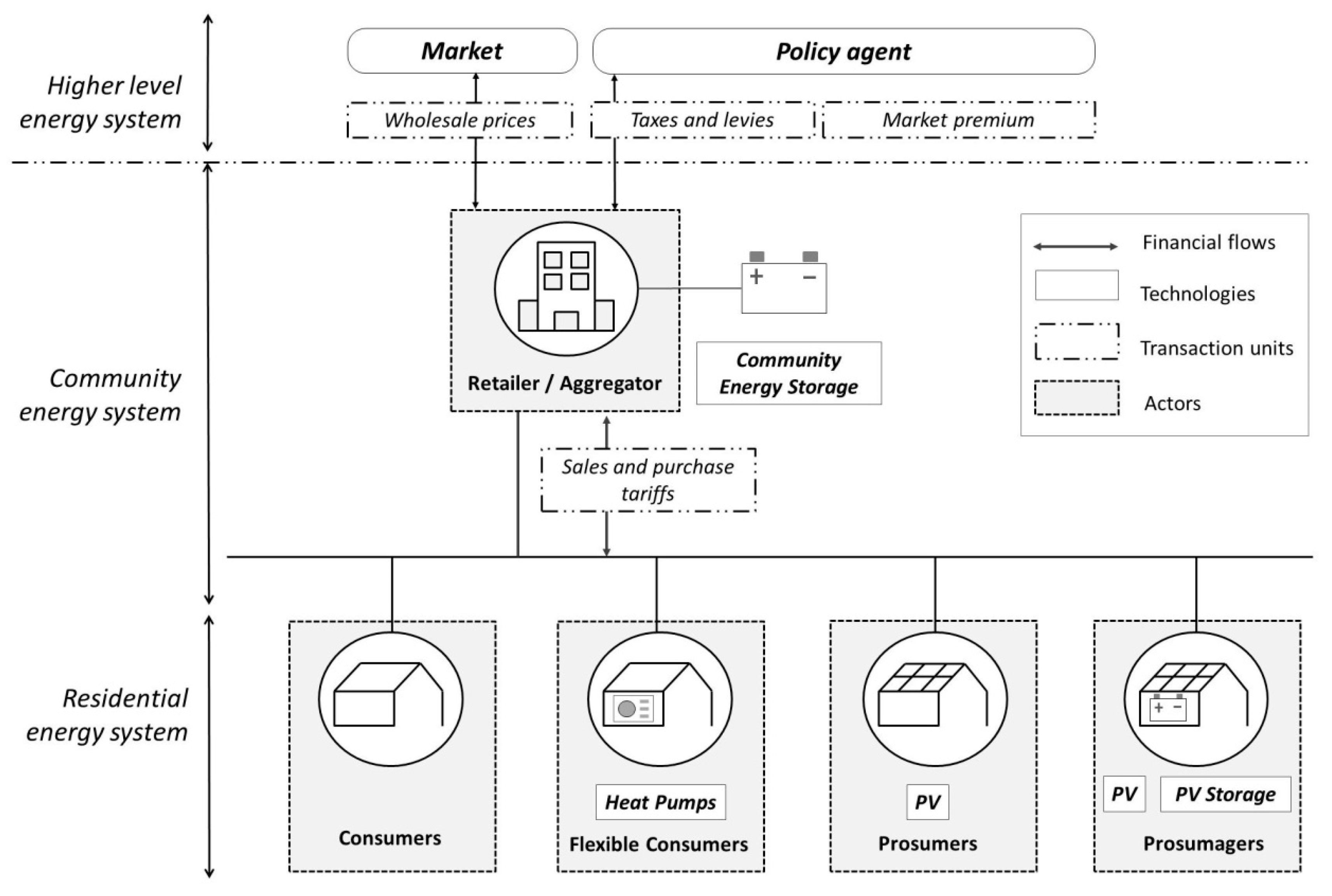
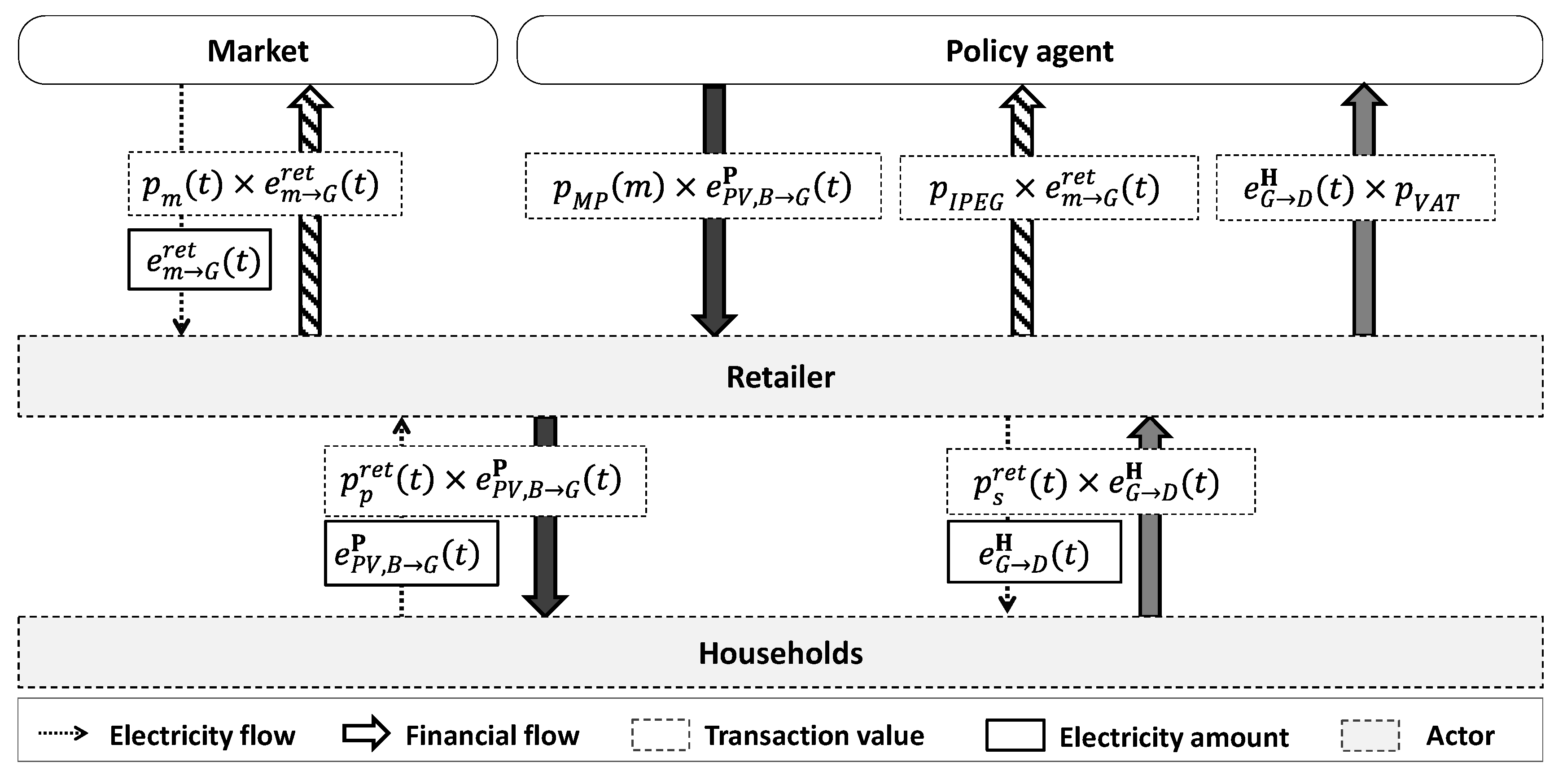
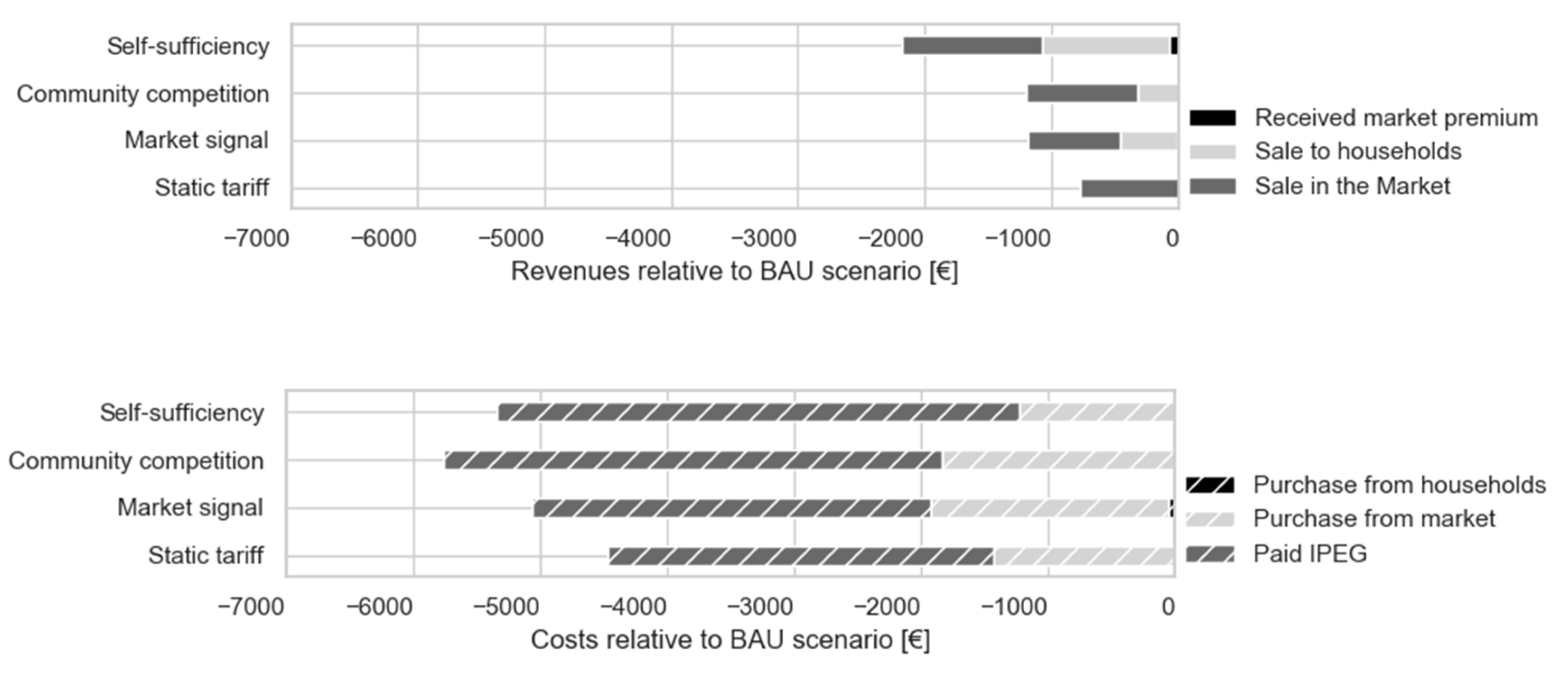
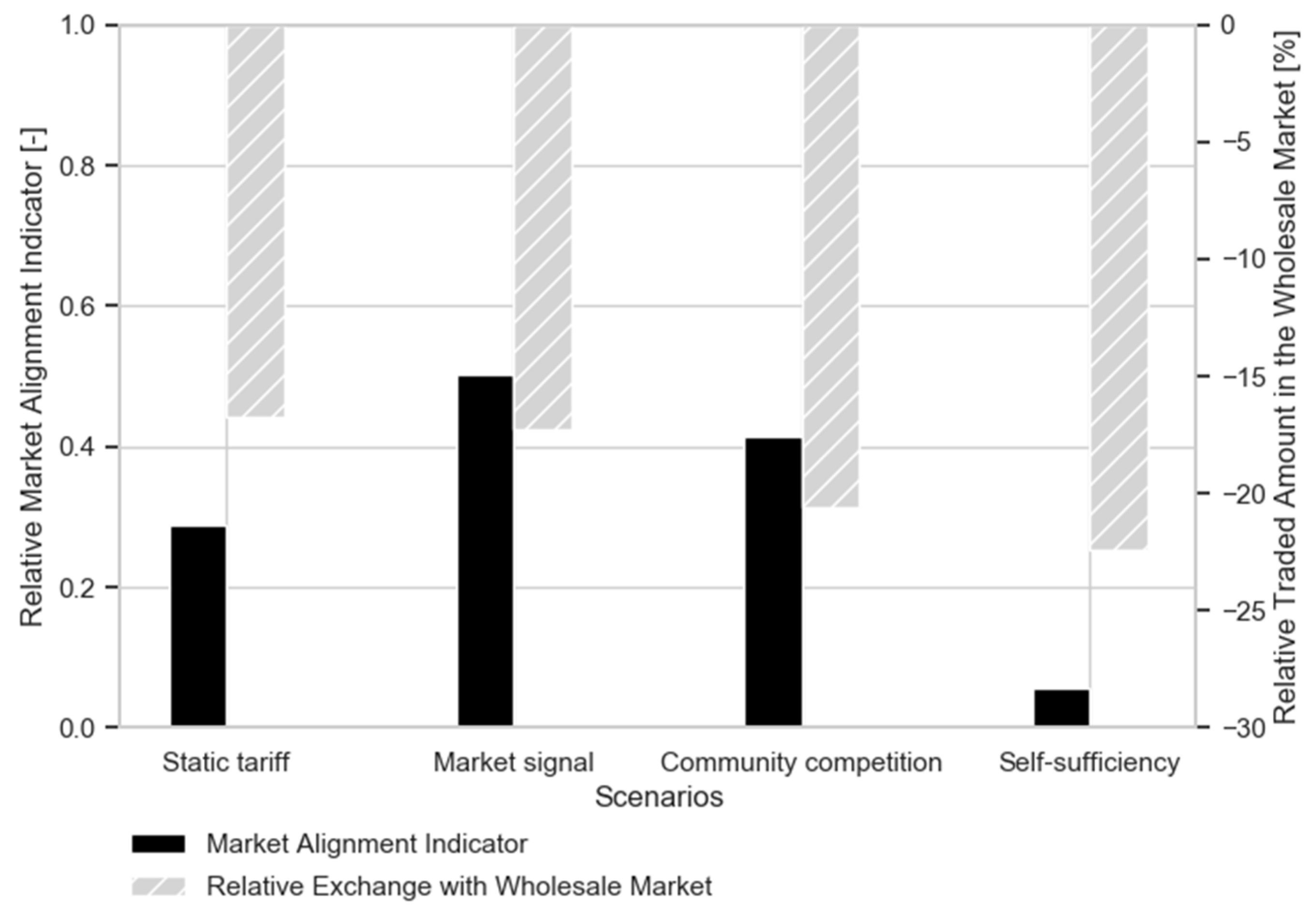
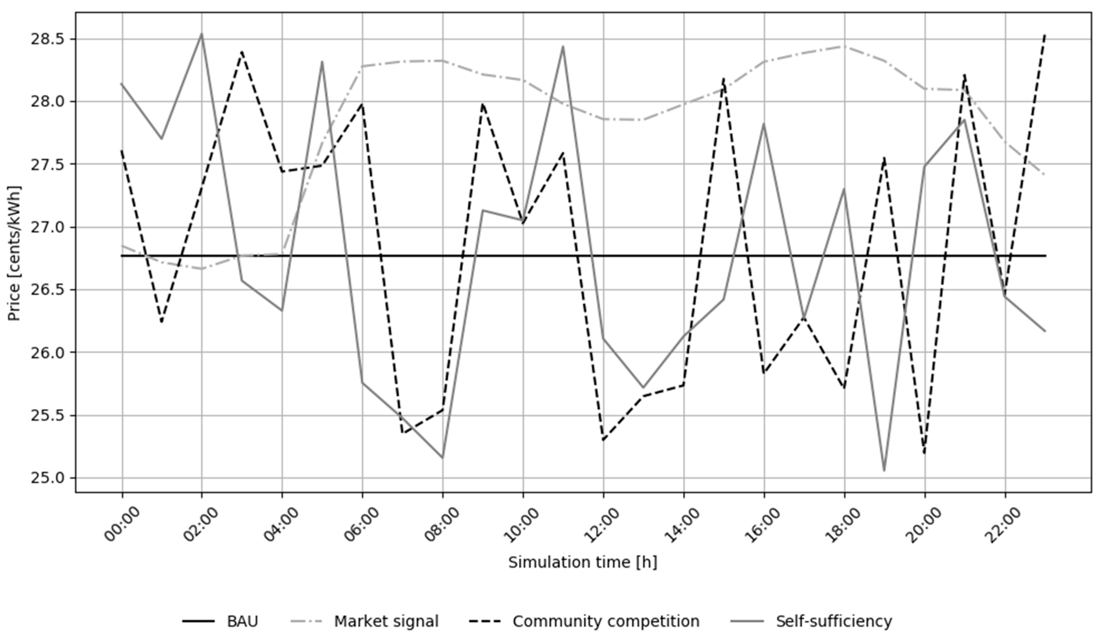
Appendix E. Electricity Prices in Different Tariffs
Figure A4 presents the electricity tariffs in the investigated scenarios for an exemplary 24 h.
Figure A4.
Electricity tariffs in the investigated scenarios for an exemplary 24 h.

The mean value and standard deviation of the electricity tariffs in different seasons are presented in Table A2 and Table A3, respectively. Since the electricity prices in the BAU scenario do not change over time, the statistics for the BAU scenario are not presented. In comparison with the community competition and self-sufficiency scenarios, the mean value and standard deviation of the electricity prices in the market signal scenario show a strong seasonality. This seasonality, which reflects the characteristics of the market prices, among others, results from the changes in the availability of renewable energy resources such as wind and sun.
Table A2.
Mean values of electricity tariffs during different seasons.
| Scenario | Jan–Mar | Apr–Jun | Jul–Sep | Oct-Dec |
|---|---|---|---|---|
| Market signal | 25.85 | 25.77 | 27.80 | 27.66 |
| Community competition | 26.86 | 26.84 | 26.82 | 26.83 |
| Self-sufficiency | 26.60 | 26.58 | 26.61 | 26.59 |
Table A3.
Standard deviation of electricity retail prices during different seasons.
| Scenario | Jan–Mar | Apr–Jun | Jul–Sep | Oct–Dec |
|---|---|---|---|---|
| Market signal | 1.98 | 1.81 | 1.48 | 2.19 |
| Community competition | 0.92 | 0.95 | 1.04 | 0.90 |
| Self-sufficiency | 0.98 | 1.00 | 1.03 | 1.01 |
Appendix F. Exemplary Dispatch Optimization Results
Appendix F.1. 48 h Flexible Consumers’ Schedule in Response to M-RTP Tariff
In the following, a closer observation of flexible consumer’s behavior in reaction to real-time pricing signals is given. Figure A5 shows the optimization results for flexible consumers during the first two days of January in response to the M-RTP tariff. It can be seen that as the heat pump shifts the load to the hours with low electricity prices, the total households’ electricity load is lower when peak prices occur. Note that the plotted data are aggregated for 10 flexible consumers.
Figure A5.
Flexible consumers’ response to the M-RTP tariff for the first 48 h in January. (A) Flexible consumers’ heat demand and electricity load; (B) state of charge of the thermal storage and electricity tariffs.
Figure A5.
Flexible consumers’ response to the M-RTP tariff for the first 48 h in January. (A) Flexible consumers’ heat demand and electricity load; (B) state of charge of the thermal storage and electricity tariffs.

Appendix F.2. 48 h Prosumagers’ Schedule in Response to M-RTP Tariff
Figure A6 shows the prosumagers’ optimization results of the first two days of January in response to the M-RTP tariff. The battery dispatch results, depicted in sub-figure B, shows that the battery during these two days did not sell electricity to the grid. When the electricity tariffs were low, the battery was used to buy electricity for later use. This can be seen clearly, for instance, on Sat 4:00. The sub-figure C demonstrates that the residual generation of the prosumagers is not fed into the grid but is rather stored in the battery (see for example Fri 12:00). Note that according to the optimization assumption, the generated electricity is first used to cover the load, and the residual generation may be sold to the grid or stored in the battery.
Figure A6.
Prosumagers’ reaction to M-RTP tariff: (A) 48h electricity tariffs and purchase prices (B) schedule details of battery systems (C) 48h usage of PV generated electricity.
Figure A6.
Prosumagers’ reaction to M-RTP tariff: (A) 48h electricity tariffs and purchase prices (B) schedule details of battery systems (C) 48h usage of PV generated electricity.

Appendix G. NPV Calculations
For the NPV calculations, the initial investment in CES can be formulated as:
where is derived from the battery module price multiplied by the size of the CES. In this calculation, we neglect the scaling effect that accounts for the lower specific cost for larger battery systems. Since in retailer’s costs and revenue streams, the operation and maintenance costs of the CES are not taken into account, we obtain the retailer’s net profit for the scenario from the following equation:
The operation and maintenance costs in this equation are considered to be a percentage (of the initial investment costs. The NPV for the scenario is then calculated as follows:
where is the discount rate and is the battery lifetime that assumed to be the project lifetime. To isolate the effect of CES in the cash flows, in the NPV calculations the retailer’s net income in the BAU scenario is subtracted from . The amount of cash flows are divided into 100 to convert the units from cents to euros.
References
- Lang, T.; Ammann, D.; Girod, B. Profitability in absence of subsidies: A techno-economic analysis of rooftop photovoltaic self-consumption in residential and commercial buildings. Renew. Energy 2016, 87, 77–87. [Google Scholar] [CrossRef]
- Bazilian, M.; Onyeji, I.; Liebreich, M.; MacGill, I.; Chase, J.; Shah, J.; Gielen, D.; Arent, D.; Landfear, D.; Zhengrong, S. Re-considering the economics of photovoltaic power. Renew. Energy 2013, 53, 329–338. [Google Scholar] [CrossRef]
- Agnew, S.; Dargusch, P. Effect of residential solar and storage on centralized electricity supply systems. Nat. Clim. Chang. 2015, 5, 315. [Google Scholar] [CrossRef]
- Cole, W.J.; Frazier, A. Cost Projections for Utility-Scale Battery Storage; National Renewable Energy Lab.(NREL): Golden, CO, USA, 2019.
- Hoppmann, J.; Volland, J.; Schmidt, T.S.; Hoffmann, V.H. The economic viability of battery storage for residential solar photovoltaic systems–A review and a simulation model. Renew. Sustain. Energy Rev. 2014, 39, 1101–1118. [Google Scholar] [CrossRef]
- Bertsch, V.; Geldermann, J.; Lühn, T. What drives the profitability of household PV investments, self-consumption and self-sufficiency? Appl. Energy 2017, 204, 1–15. [Google Scholar] [CrossRef] [Green Version]
- Ruhnau, O.; Bannik, S.; Otten, S.; Praktiknjo, A.; Robinius, M. Direct or indirect electrification? A review of heat generation and road transport decarbonisation scenarios for Germany 2050. Energy Build. 2019, 166, 989–999. [Google Scholar] [CrossRef] [Green Version]
- Dehler, J.; Keles, D.; Telsnig, T.; Fleischer, B.; Baumann, M.; Fraboulet, D.; Faure-Schuyer, A.; Fichtner, W. Self-consumption of electricity from renewable sources. In Europe’s Energy Transition-Insights for Policy Making; Elsevier: Amsterdam, The Netherlands, 2017; pp. 225–236. [Google Scholar]
- Schill, W.-P.; Zerrahn, A.; Kunz, F. Prosumage of Solar Electricity: Pros, Cons, and the System Perspective. 2017. Available online: https://papers.ssrn.com/sol3/papers.cfm?abstract_id=2912814 (accessed on 7 February 2017). [CrossRef] [Green Version]
- Klein, M.; Ziade, A.; De Vries, L. Aligning prosumers with the electricity wholesale market–The impact of time-varying price signals and fixed network charges on solar self-consumption. Energy Policy 2019, 134, 110901. [Google Scholar] [CrossRef]
- Pudjianto, D.; Ramsay, C.; Strbac, G. Virtual power plant and system integration of distributed energy resources. IET Renew. Power Gener. 2007, 1, 10–16. [Google Scholar] [CrossRef]
- Frieden, D.; Tuerk, A.; Roberts, J.; D’Hebermont, S.; Gubina, A. Collective Self-Consumption and Energy Communities: Overview of Emerging Regulatory Approaches in Europe. 2019. Available online: https://www.compile-project.eu/wp-content/uploads/COMPILE_Collective_self-consumption_EU_review_june_2019_FINAL-1.pdf (accessed on 15 July 2020).
- Roberts, J.; Frieden, D.; d’Herbemont, S. Energy Community Definitions. Deliverable Developed Under the Scope of the COMPILE Project: Integrating Community Power in Energy Islands. 2019. Available online: https://www.compile-project.eu/wp-content/uploads/Explanatory-note-on-energy-community-definitions.pdf (accessed on 5 December 2019).
- Koirala, B.P.; Koliou, E.; Friege, J.; Hakvoort, R.A.; Herder, P.M. Energetic communities for community energy: A review of key issues and trends shaping integrated community energy systems. Renew. Sustain. Energy Rev. 2016, 56, 722–744. [Google Scholar] [CrossRef] [Green Version]
- Deutscher Genossenschafts-und Raiffeisenverband e. V. (DGRV). Energy Cooperatives: Results of the DGRV-Survey (at 31 December 2018). Available online: https://www.dgrv.de/weben.nsf/web/annualsurveyenergycooperatives (accessed on 5 June 2019).
- Gaudchau, E.; Resch, M.; Zeh, A. Quartierspeicher: Definition, rechtlicher Rahmen und Perspektiven. Ökologisches Wirtsch.-Fachz. 2016, 31, 26–27. [Google Scholar] [CrossRef]
- Koirala, B.P.; van Oost, E.; van der Windt, H. Community energy storage: A responsible innovation towards a sustainable energy system? Appl. Energy 2018, 231, 570–585. [Google Scholar] [CrossRef]
- van der Stelt, S.; AlSkaif, T.; van Sark, W. Techno-economic analysis of household and community energy storage for residential prosumers with smart appliances. Appl. Energy 2018, 209, 266–276. [Google Scholar] [CrossRef]
- Gissey, G.C.; Dodds, P.E.; Radcliffe, J. Market and regulatory barriers to electrical energy storage innovation. Renew. Sustain. Energy Rev. 2018, 82, 781–790. [Google Scholar] [CrossRef]
- Scheller, F.; Götz, M.; Burgenmeister, B.; Seim, S.; Haberland, R.; Kondziella, H.; Bruckner, T. Legal Framework and Economic Feasibility of Neighborhood Energy Storage Systems. In Proceedings of the 10th Internationale Energiewirtschaftstagung Conference, Wien, Austria, 15 February 2017. [Google Scholar]
- Parra, D.; Swierczynski, M.; Stroe, D.I.; Norman, S.A.; Abdon, A.; Worlitschek, J.; O’Doherty, T.; Rodrigues, L.; Gillott, M.; Zhang, X. An interdisciplinary review of energy storage for communities: Challenges and perspectives. Renew. Sustain. Energy Rev. 2017, 79, 730–749. [Google Scholar] [CrossRef]
- Arghandeh, R.; Woyak, J.; Onen, A.; Jung, J.; Broadwater, R.P. Economic optimal operation of Community Energy Storage systems in competitive energy markets. Appl. Energy 2014, 135, 71–80. [Google Scholar] [CrossRef] [Green Version]
- Lombardi, P.; Schwabe, F. Sharing economy as a new business model for energy storage systems. Appl. Energy 2017, 188, 485–496. [Google Scholar] [CrossRef]
- Chakraborty, P.; Baeyens, E.; Poolla, K.; Khargonekar, P.P.; Varaiya, P. Sharing storage in a smart grid: A coalitional game approach. IEEE Trans. Smart Grid 2018, 10, 4379–4390. [Google Scholar] [CrossRef] [Green Version]
- Mediwaththe, C.P.; Stephens, E.R.; Smith, D.B.; Mahanti, A. Competitive energy trading framework for demand-side management in neighborhood area networks. IEEE Trans. Smart Grid 2017, 9, 4313–4322. [Google Scholar] [CrossRef] [Green Version]
- Liu, N.; Cheng, M.; Yu, X.; Zhong, J.; Lei, J. Energy-sharing provider for PV prosumer clusters: A hybrid approach using stochastic programming and stackelberg game. IEEE Trans. Ind. Electron. 2018, 65, 6740–6750. [Google Scholar] [CrossRef]
- Tushar, W.; Chai, B.; Yuen, C.; Smith, D.B.; Poor, H.V. Energy management for a user interactive smart community: A Stackelberg game approach. In Proceedings of the 2014 IEEE Innovative Smart Grid Technologies-Asia (ISGT ASIA) of Conference, Kuala Lumpur, Malaysia, 20–23 May 2014. [Google Scholar]
- Liu, N.; Yu, X.; Wang, C.; Wang, J. Energy sharing management for microgrids with PV prosumers: A Stackelberg game approach. IEEE Trans. Ind. Inform. 2017, 13, 1088–1098. [Google Scholar] [CrossRef]
- BDEW—Bundesverband der Energie- und Wasserwirtschaft e. V. Strompreisanalyse Januar 2020. Available online: https://www.bdew.de/media/documents/20200107_BDEW-Strompreisanalyse_Januar_2020.pdf (accessed on 1 February 2020).
- Purkus, A.; Gawel, E.; Deissenroth, M.; Nienhaus, K.; Wassermann, S. Der Beitrag der Marktprämie zur Marktintegration Erneuerbarer Energien–Erfahrungen aus dem EEG 2012 und Perspektiven der Verpflichtenden Direktvermarktung; Helmholtz-Zentrum für Umweltforschung—UFZ: Leipzig, Germany, 2017; Available online: http://hdl.handle.net/10419/102740 (accessed on 5 June 2020).
- Sterner, M.; Stadler, I. Energiespeicher-Bedarf, Technologien, Integration; Springer: Berlin, Germany, 2014. [Google Scholar]
- Winkler, J.; Sensfuß, F.; Pudlik, M. Leitstudie Strommarkt Arbeitspaket 4 Analyse Ausgewählter Einflussfaktoren auf den Marktwert Erneuerbarer Energien. 2015. Available online: https://www.bmwi.de/Redaktion/DE/Publikationen/Studien/leitstudie-strommarkt_analyse-ausgewaehlter-einflussfaktoren-auf-den-martkwert-erneuerbarer-energien.pdf?__blob=publicationFile&v=3 (accessed on 27 March 2020).
- Gawel, E.; Purkus, A. EEG 2017—Mehr Markt bei der Erneuerbare-Energien-Förderung? Wirtschaftsdienst 2016, 96, 910–915. [Google Scholar] [CrossRef] [Green Version]
- Maly, D.K.; Kwan, K.-S. Optimal battery energy storage system (BESS) charge scheduling with dynamic programming. IEE Proc. Sci. Meas. Technol. 1995, 142, 453–458. [Google Scholar] [CrossRef]
- Open Power System Data: Data Package Time Series. 2019. Available online: https://windenergyscience.com/learn-and-thrive/time-series-data/ (accessed on 27 March 2020). [CrossRef]
- Netztransparenz, Marktwertübersicht. Available online: https://www.netztransparenz.de/EEG/Marktpraemie/Marktwerte (accessed on 5 May 2019).
- Bundesverband Solarwirtschaft eV Feste Einspeise-Vergütungen im Überblick. 2017. Available online: https://www.solarwirtschaft.de/fileadmin/user_upload/Verguetungsuebersicht-Basis.pdf (accessed on 12 January 2020).
- Tjaden, T.; Bergner, J.; Weniger, J.; Quaschning, V. Repräsentative Elektrische Lastprofile für Wohngebäude in Deutschland auf 1-sekündiger Datenbasis; Hochschule für Technik und Wirtschaft HTW Berlin: Berlin, Germany, 2015. [Google Scholar]
- Hayn, M.; Zander, A.; Fichtner, W.; Nickel, S.; Bertsch, V.J.E.S. The impact of electricity tariffs on residential demand side flexibility: Results of bottom-up load profile modeling. Energy Syst. 2018, 9, 759–792. [Google Scholar] [CrossRef]
- Ruhnau, O. When2Heat Heating Profiles. Open Power Syst. Data 2019. [Google Scholar] [CrossRef]
- Ruhnau, O.; Hirth, L.; Praktiknjo, A. Time series of heat demand and heat pump efficiency for energy system modeling. Sci. Data 2019, 6, 189. [Google Scholar] [CrossRef]
- Engelken, M.; Römer, B.; Drescher, M.; Welpe, I. Why homeowners strive for energy self-supply and how policy makers can influence them. Energy Policy 2018, 117, 423–433. [Google Scholar] [CrossRef]
- Förster, H.; Kunert, D.; Hünecke, K.; Schumacher, K.; Siemons, A.; Zell-Ziegler, C. Hintergrundpapier: 50 Jahre Mehrwertsteuer–Ein Blick durch die Klimaschutzbrille. Available online: https://www.oeko.de/fileadmin/oekodoc/Hintergrundpapier_Mehrwertsteuer_2018.pdf (accessed on 18 April 2020).
- Khalid, A.M.; Mitra, I.; Warmuth, W.; Schacht, V. Performance ratio–Crucial parameter for grid connected PV plants. Renew. Sustain. Energy Rev. 2016, 65, 1139–1158. [Google Scholar] [CrossRef]
- Forsén, M.; Boeswarth, R.; Dubuisson, X.; Sandström, B. Heat Pumps: Technology and Environmental Impact. Swedish Heat Pump Association (SVEPR). 2005. Available online: https://ec.europa.eu/environment/ecolabel/about_ecolabel/reports/hp_tech_env_impact_aug2005.pdf (accessed on 3 November 2019).
- Thomann, R.; Lachmann, Y.; Prahl, O. Strombank: Innovatives Betreibermodell für Quartierspeicher. 2016. Available online: https://www.mvv.de/fileadmin/user_upload/Ueber_uns/de/Strombank_Abschlussbericht_2016.pdf (accessed on 12 June 2020).
- Schick, C.; Blesl, M.; Borggrefe, F.; Brand, H.; Buchmann, T.; Fahl, U.; Fuchs, A.-L.; Gils, H.; Hufendiek, K.; Münkel, A.; et al. Energiesystemanalyse Baden-Württemberg; Ministerium für Umwelt, Klima und Energiewirtschaft Baden-Württemberg: Stuttgart, Germany, 2018. [Google Scholar]
- Meng, F.-L.; Zeng, X.-J. An optimal real-time pricing for demand-side management: A Stackelberg game and genetic algorithm approach. In Proceedings of the 2014 International Joint Conference on Neural Networks (IJCNN) of Conference, Beijing, China, 6–11 July 2014. [Google Scholar]
- Hejazi, S.R.; Memariani, A.; Jahanshahloo, G.; Sepehri, M.M. Linear bilevel programming solution by genetic algorithm. Comput. Oper. Res. 2002, 29, 1913–1925. [Google Scholar] [CrossRef]
- Wilhelmstötter, F. JENETICS Library User’s Manual 4.3. 2016. Available online: http://jenetics.io/ (accessed on 20 July 2020).
- Braeuer, F.; Kleinebrahm, M.; Naber, E. Effects of the tenants electricity law on energy system layout and landlord-tenant relationship in a multi-family building in Germany. In Proceedings of the IOP Conference Series: Earth and Environmental Science of Conference, Graz, Austria, 11–14 September 2019. [Google Scholar]
- Gährs, S.; Knoefel, J.; Cremer, N. Politische Zielsetzungen und Rechtlicher Rahmen für Quartierspeicher. 2017, p. 2019. Available online: https://www.esquire-projekt.de/data/esquire/Datein/Arbeitspapier_Politische_Zielsetzungen_und_rechtlicher_Rahmen_f%C3%BCr_Quartierspeicher.pdf (accessed on 25 January 2020).
- Schwarz, H.; Schermeyer, H.; Bertsch, V.; Fichtner, W. Self-consumption through power-to-heat and storage for enhanced PV integration in decentralised energy systems. Solar Energy 2018, 163, 150–161. [Google Scholar] [CrossRef] [Green Version]
- Neuteleers, S.; Mulder, M.; Hindriks, F. Assessing fairness of dynamic grid tariffs. Energy Policy 2017, 108, 111–120. [Google Scholar] [CrossRef] [Green Version]
- Förderer, K.; Lösch, M.; Növer, R.; Ronczka, M.; Schmeck, H. Smart Meter Gateways: Options for a BSI-Compliant Integration of Energy Management Systems. Appl. Sci. 2019, 9, 1634. [Google Scholar] [CrossRef] [Green Version]
- Gesetz Über Den Messstellenbetrieb und Die Datenkommunikation in Intelligenten Energienetzen (Messstellenbetriebsgesetz–MsbG). 2016, Volume 2, p. 48. Available online: https://www.gesetze-im-internet.de/messbg/MsbG.pdf (accessed on 7 February 2020).
- Khalilpour, R.; Vassallo, A. Leaving the grid: An ambition or a real choice? Energy Policy 2015, 82, 207–221. [Google Scholar] [CrossRef]
- Kaschub, T.; Jochem, P.; Fichtner, W. Solar energy storage in German households: Profitability, load changes and flexibility. Energy Policy 2016, 98, 520–532. [Google Scholar] [CrossRef] [Green Version]
- Simshauser, P. Distribution network prices and solar PV: Resolving rate instability and wealth transfers through demand tariffs. Energy Econ. 2016, 54, 108–122. [Google Scholar] [CrossRef]
- Parra, D.; Gillott, M.; Norman, S.A.; Walker, G.S. Optimum community energy storage system for PV energy time-shift. Appl. Energy 2015, 137, 576–587. [Google Scholar] [CrossRef]
- Ensslen, A.; Ringler, P.; Dörr, L.; Jochem, P.; Zimmermann, F.; Fichtner, W. Incentivizing smart charging: Modeling charging tariffs for electric vehicles in German and French electricity markets. Energy Res. Soc. Sci. 2018, 42, 112–126. [Google Scholar] [CrossRef]
- Maharjan, S.; Zhu, Q.; Zhang, Y.; Gjessing, S.; Basar, T. Dependable demand response management in the smart grid: A Stackelberg game approach. IEEE Trans. Smart Grid 2013, 4, 120–132. [Google Scholar] [CrossRef]
- Alabdullatif, A.M.; Gerding, E.H.; Perez-Diaz, A.J.E. Market Design and Trading Strategies for Community Energy Markets with Storage and Renewable Supply. Energies 2020, 13, 972. [Google Scholar] [CrossRef] [Green Version]
- ALSalloum, H.; ELMasri, A.; Merghem-Boulahia, L.; Rahim, R. Demand side management in smart grids: A stackelberg multi period multi provider game. In Proceedings of the 2018 9th IFIP International Conference on New Technologies, Mobility and Security (NTMS) of Conference, Paris, France, 26–28 February 2018. [Google Scholar]
- Bellman, R.E.; Dreyfus, S.E. Applied Dynamic Programming; Princeton University Press: Princeton, NJ, USA, 2015. [Google Scholar]
Figure 1.
Community Energy Storage (CES) business models as a complex socio-technical system (own presentation based on [12]).
Figure 1.
Community Energy Storage (CES) business models as a complex socio-technical system (own presentation based on [12]).

Figure 2.
Schematic overview of the community energy system model.

Figure 3.
Overview of the regulatory induced financial flows in the model. Arrows with similar patterns or color show related financial flows.
Figure 3.
Overview of the regulatory induced financial flows in the model. Arrows with similar patterns or color show related financial flows.

Figure 4.
Energy flows in the flexible consumers’ model.

Figure 5.
Schematic sketch of the prosumagers’ model.

Figure 6.
Two-level Stackelberg game structure in the C-RTP tariff.

Figure 7.
The duration curve of electricity tariffs in different scenarios.

Figure 8.
Actor’s utilities relative to BAU scenario. A positive value indicates an increase in the net income, negative values represent a decrease in net income.
Figure 8.
Actor’s utilities relative to BAU scenario. A positive value indicates an increase in the net income, negative values represent a decrease in net income.

Figure 9.
Retailer’s cost and revenue streams relative to the BAU scenario; negative values show the reduction of each stream relative to the corresponding stream in the BAU scenario.
Figure 9.
Retailer’s cost and revenue streams relative to the BAU scenario; negative values show the reduction of each stream relative to the corresponding stream in the BAU scenario.

Figure 10.
Community welfare in comparison to the BAU case.

Figure 11.
Relative market alignment indicator and reduced exchange with market compared to the BAU scenario.
Figure 11.
Relative market alignment indicator and reduced exchange with market compared to the BAU scenario.

Table 1.
Overview of constructed tariff structures.
| Tariff | Real-Time Component | |
|---|---|---|
| SP | None | |
| M-RTP | , exogenous model input | |
| C-RTP | , derived endogenously (See Section 3.3) |
Table 2.
Scenarios.
| Scenario | Tariff | Aggregation Goal |
|---|---|---|
| Business As Usual (BAU)—no storage | SP | None |
| Static tariff | SP | Maximum profit |
| Market signal | M-RTP | Maximum profit |
| Community competition | C-RTP | Maximum profit |
| Self-sufficiency | C-RTP | Maximum self-sufficiency |
Table 3.
Descriptive statistics of the households’ demand time series.
| Input Parameter | Unit | Resolution | Mean | Min | Max | Total |
|---|---|---|---|---|---|---|
| Electricity demand () | kWh | Hour | 0.53 | 0.19 | 1.33 | 4685 |
| Heat demand ( | kWh | Hour | 2.28 | 0.12 | 7.17 | 19,996 |
Table 4.
Model parameters.
| Parameter | Unit | Value | Source |
|---|---|---|---|
| cent/kWh | 12.3 | German Solar Association [37] | |
| cent/kWh | 7.68 | BDEW [29] | |
| cent/kWh | 7.3 | BDEW [29] | |
| cent/kWh | 3.71 | BDEW [29] | |
| cent/kWh | 18 | Model assumption | |
| VAT | % | 19 | Förster et al. [43] |
| kW | 6 | Model assumption | |
| % | 84 | Khalid et al. [44] | |
| kWh | 6 | Model assumption | |
| kW | 8 | Model assumption | |
| - | 3 | Forsén et al. [45] | |
| kWh | 14 | Model assumption | |
| kWh | 100 | Thorman et al. [46] | |
| % | 95 | Klein et al. [10] | |
| % | 95 | Klein et al. [10] | |
| - | 1 | Thorman et al. [46] | |
| % | 1 | Klein et al. [10] | |
| % | 4 | Model assumption | |
| years | 20 | Model assumption | |
| €/kWh | 510 and 250 | Schick et al. [47] | |
| hours | 24 | Model assumption | |
| hours | 8760 | Model assumption |
Table 5.
GA parameters; the detailed description of the parameters can be found in [50].
Table 5.
GA parameters; the detailed description of the parameters can be found in [50].
| Parameter | Value |
|---|---|
| Population size | 60 |
| Offspring fraction | 0.2 |
| Mutation | 0.6 |
| Single point crossover | 1 |
| Population convergence threshold | 0.01% |
Table 6.
Scenario-specific statistic values of electricity tariffs.
| Scenario | Tariff | Mean Value [cents] | Standard Deviation [-] | Price Range 1 [cents] |
|---|---|---|---|---|
| BAU/Static tariff | SP | 26.76 | 0 | [26.76, 26.76] |
| Market signal | M-RTP | 26.76 | 2.09 | [14.40, 36.68] |
| Community competition | C-RTP | 26.83 | 0.96 | [24.99, 28.56] |
| Self-sufficiency | C-RTP | 26.58 | 1.01 | [24.99, 28.56] |
1 The price range shows the minimum and maximum values of the electricity tariffs during the simulation time.
Table 7.
Changes in the community energy system’s import and export 1.
| Scenario | Relative Import (%) | Relative Export (%) |
|---|---|---|
| Static tariff | −9.6 | −45.0 |
| Market signal | −9.9 | −46.3 |
| Community competition | −12.4 | −53.1 |
| Self-sufficiency | −13.0 | −59.5 |
1 Relative electricity import and export refers to the purchased and sold electricity in the market by the retailer relative to the corresponding values in the BAU scenario.
Table 8.
NPV for different aggregation scenarios 1.
| Scenario | Unit | NPV_510 | NPV_250 |
|---|---|---|---|
| Static tariff | € | −17,280.1 | 16,512.9 |
| Market signal | € | −13,795.8 | 19,997.2 |
| Community competition | € | −11,671.7 | 22,121.4 |
| Self-sufficiency | € | −27,043.5 | 6749.5 |
1 NPV_510 and NPV_250 refer to the NPVs for battery prices of 510 and 250 (€/kWh) respectively.
Table 9.
Collected EEG levy and grid charges by the policy agent relative to the BAU scenario.
| Scenario | Grid Charges (€) | EEG Levy (€) |
|---|---|---|
| Static tariff | −1202.51 | −1120.15 |
| Market signal | −1242.57 | −1157.46 |
| Community competition | −1551.29 | −1445.03 |
| Self-sufficiency | −1628.25 | −1516.72 |
© 2020 by the authors. Licensee MDPI, Basel, Switzerland. This article is an open access article distributed under the terms and conditions of the Creative Commons Attribution (CC BY) license (http://creativecommons.org/licenses/by/4.0/).
Share and Cite
MDPI and ACS Style
Sarfarazi, S.; Deissenroth-Uhrig, M.; Bertsch, V. Aggregation of Households in Community Energy Systems: An Analysis from Actors’ and Market Perspectives. Energies 2020, 13, 5154. https://0-doi-org.brum.beds.ac.uk/10.3390/en13195154
AMA Style
Sarfarazi S, Deissenroth-Uhrig M, Bertsch V. Aggregation of Households in Community Energy Systems: An Analysis from Actors’ and Market Perspectives. Energies. 2020; 13(19):5154. https://0-doi-org.brum.beds.ac.uk/10.3390/en13195154
Chicago/Turabian StyleSarfarazi, Seyedfarzad, Marc Deissenroth-Uhrig, and Valentin Bertsch. 2020. "Aggregation of Households in Community Energy Systems: An Analysis from Actors’ and Market Perspectives" Energies 13, no. 19: 5154. https://0-doi-org.brum.beds.ac.uk/10.3390/en13195154
Note that from the first issue of 2016, this journal uses article numbers instead of page numbers. See further details here.