Next-Day Prediction of Hourly Solar Irradiance Using Local Weather Forecasts and LSTM Trained with Non-Local Data


Department of Architectural Engineering, Inha University, Incheon 22212, Korea
*
Author to whom correspondence should be addressed.
Energies 2020, 13(20), 5258; https://0-doi-org.brum.beds.ac.uk/10.3390/en13205258
Submission received: 18 September 2020
/
Revised: 28 September 2020
/
Accepted: 2 October 2020
/
Published: 10 October 2020
(This article belongs to the Special Issue Energy-Saving, Comfort, and Healthier Strategies for Smart Buildings)
Abstract
:Solar irradiance prediction is significant for maximizing energy-saving effects in the predictive control of buildings. Several models for solar irradiance prediction have been developed; however, they require the collection of weather data over a long period in the predicted target region or evaluation of various weather data in real time. In this study, a long short-term memory algorithm–based model is proposed using limited input data and data from other regions. The proposed model can predict solar irradiance using next-day weather forecasts by the Korea Meteorological Administration and daily solar irradiance, and it is possible to build a model with one-time learning using national and international data. The model developed in this study showed excellent predictive performance with a coefficient of variation of the root mean square error of 12% per year even if the learning and forecast regions were different, assuming that the weather forecast was correct.
1. Introduction
In general, approximately 60% of a building’s energy is used for heating, ventilation, and air conditioning operation [1], and energy can be saved by optimally controlling the building’s heating and air conditioning systems [2]. There have been an increasing number of studies related to model predictive control (MPC), which establishes an optimal control strategy to ensure efficient air conditioner control and system operation in advance [3,4]. Various studies have confirmed the effect of reducing building energy consumption through MPC [5,6,7]. The performance of MPC control is affected by the accuracy of the hourly load prediction of a building, and the load is affected by next-day weather information; therefore, most models require weather forecast information [8,9,10]. Typical factors affecting the load are outdoor air temperature and solar irradiance. Although prediction of outdoor air temperature is relatively easy because of small hourly changes, forecasting the actual hourly values of solar irradiance is very rare [11,12,13,14]. In previous MPC studies, methods of predicting solar irradiance have been rarely reported, and most studies were conducted using the data provided by an energy analysis program or assuming that the amount of solar irradiance was completely predicted from the solar irradiance prediction model [15].
Solar irradiance prediction models are typically physics-based or data-based [16]. Physical models are generally developed based on solar geometry to construct an empirical correlation between solar irradiance data and meteorological parameters measured in the past in the observation region [17]. In 1956, the author Black developed a model for predicting solar irradiance by analyzing the correlation between sky cover and solar irradiance data measured over three years in a region [18]. Similarly, Samimi developed a solar irradiance model with high accuracy using Iran’s weather data measured over 17 years [19]. Paltridge and Daneshyar [20,21] developed physics-based solar irradiance prediction models using various weather parameters such as humidity, wind, and precipitation, and long-term accumulated data. However, according to Premalatha and Valan, to describe solar irradiance coefficients in a local region, physics-based weather forecasting prediction models require long-term measurement data or data that are difficult to secure from general weather forecast information [22]. Therefore, the model cannot be applied for predicting next-day solar irradiance. A solar irradiance model based on the physical model was developed for calculating monthly or annual total solar irradiance, rather than a real-time prediction model, such as a model for MPC applications [23].
Another method of solar irradiance prediction is the application of machine learning techniques, such as artificial neural networks (ANNs) and deep learning, without using physical models, and the number of studies in which these techniques are used has been steadily increasing. Lago et al. [24] reported that neural network structures are advantageous for learning and predicting time-series data with high randomness, and Jiang [25] reported that the ANN prediction model exhibits higher accuracy than the empirical physical solar irradiance prediction model. The solar irradiance prediction model, which was developed based on learning data, incorporates various learning methods depending on the purpose. Sharma et al. [26] developed a model that learned at 15 min intervals, and Kemoku et al. conducted a study to predict next-day solar irradiance by learning solar irradiance data for the past six years in Japan through a feedforward neural network [27]. Ahmad et al. [28] conducted a study to identify the optimal combination of input parameters favorable to prediction through experiments involving weather parameter combinations of 12 cases of solar irradiance prediction in New Zealand. Furthermore, Benmouiza and Cheknane [29] proposed a learning model for solar irradiance prediction that mixed different types of ANNs. Research on ANN-based solar irradiance prediction has been conducted extensively, and recently, a prediction model that does not use data obtained from the ground has been developed. To predict local solar irradiance, Linares et al. [30] developed an ANN model that learns data, obtained from satellites, for 6 years measured in various regions. Srivastava [31] also developed a solar irradiance prediction model that learns a significant amount of data pertaining to several European cities and obtained from satellites. The model was used to study 9-year weather patterns in 21 cities in the US and Europe. In addition, there are various learning-based solar irradiance prediction models, and Voyant et al. [32] reviewed the latest research and techniques for solar irradiance prediction.
However, according to Qing [33], these solar irradiance prediction models are difficult to use for controlling residential buildings or small- and medium-sized buildings. This is because solar irradiance models can be effectively used only by large-scale operators because historical solar irradiance and meteorological data, which are the input data of the learning model, require expensive equipment to measure for a sufficient period in one region and are continuously collected. Thus, the existing solar irradiance prediction models must be improved to allow the application of the aforementioned prediction control algorithms, such as MPC. Therefore, Qing developed a solar irradiance model that predicts solar irradiance by improving the simple solar irradiance prediction model using only the weather forecast system that is easily available through the long short-term memory (LSTM) deep learning algorithm, which is advantageous for predicting time-series data. In Qing’s study, relatively small amounts of local data were used; however, it is still difficult to use the model without data measured in the corresponding region before the MPC application because it is essential to collect solar irradiance data in the local region in the pre-prediction learning phase.
Previous solar irradiance prediction models are difficult to use directly as a building energy model for prediction control because the input data of most of these models are the detailed data from the weather measurement center, not the weather forecast system. Additionally, as they require data measured over a long time in a specific region, it is difficult to apply MPC in a region where there are no accumulated local data.
Therefore, in this study, we aimed to develop a solar irradiance prediction model to achieve optimal operation for small residential buildings and renewable energy generators using the LSTM model, which showed excellent predictive performance in previous studies. First, we intended to develop a learning model that reflects the recent solar irradiance characteristics of the surrounding region without long-term accumulated data of the predicted region. Second, we intended to develop a prediction model that can be used without additional updates with only one learning, considering the performance of the embedded central processing unit (CPU) installed in the controller of a small- to medium-sized building. Finally, we used only weather forecast information that could be easily accessed from a mobile device or PC and considered a simple weather forecast to increase the analysis efficiency by using a data collection environment that mirrors the actual environment.
2. Development of the LSTM Solar Irradiance Prediction Model
2.1. LSTM Networks
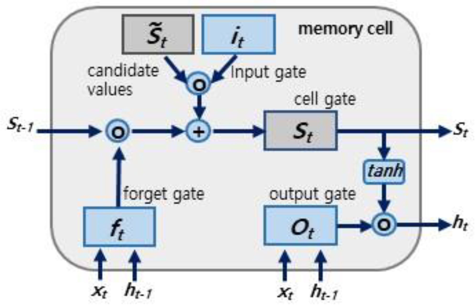
In this study, a solar irradiance prediction model was developed using a deep learning structure. In this structure, a specific neural network structure responsible for learning was defined in multiple layers and typically classified into a convolutional neural network (CNN) structure and a recurrent neural network (RNN) structure. The CNN structure exhibits excellent learning ability for information whose order is not important, such as images, and the RNN structure has been verified in many studies to learn successfully and predict problems with time-series characteristics or order [34]. In this study, the model learns using RNN because the solar irradiance in the previous period also has a time-series characteristic that moderately affects the next period. However, in the existing RNN, when learning increases, a vanishing and exploding problem [35] occurs that does not improve learning performance. The LSTM network can improve existing RNNs [36] and consists of one input layer, multiple hidden layers, and one output layer. The input and output layers are constructed in the same form as the existing neuron network model and have a number of neurons that correspond to the data size of the input and output variables. The main feature of the LSTM model is the hidden layer with memory cells. The structure of the memory cell is shown in Figure 1.
Each memory cell maintains or adjusts the cell state through three gates and is composed of an input gate , an output gate , and a forget gate . The purpose of each gate is as follows [38].
- -
- Input gate: specifies which information is added to the cell state;
- -
- Output gate: specifies which information from the cell state is used as output;
- -
- Forget gate: defines which information is removed from the cell state.
The following equations (Equations (1)–(4)) represent the process of updating memory cells in the LSTM layer at a given time step, t.
The notation definitions are as follows:
: weight matrix
: bias vector
: candidate cell-state value
: coefficient vector for the outputs of the LSTM layer
: sigmoid function
: input vector at time step t
Finally, the current cell state was determined by the following Equation (5).
Here, ∘ refers to the Hadamard product, which is an operation of multiplying co-location matrix terms between two matrices of the same size.
The output layer was calculated as the product of the current states, output gate, and , the active function. The output layer was used as a coefficient for prediction, and the output values, and are expressed by the following Equations (6) and (7):
The LSTM network equations and main contents described in this study were referenced from previous studies [33,34,35,36,37,38,39]. In this study, the LSTM model used the deep learning toolbox provided by MATLAB and specified various hyperparameters and algorithms that determine learning performance. First, the stochastic gradient descent (SGD) algorithm and adaptive moment estimation (ADAM) algorithm were used as optimization techniques provided by MATLAB. It is known that the SGD algorithm has a disadvantage because it takes a long time to learn when a sufficient working environment for iterative calculation is not provided [40]. The ADAM algorithm is advantageous for identifying the optimal solution efficiently in a short time by flexibly adjusting the learning rate [41].
The mathematical formalism and calculation process on ADAM are detailed in the reference [42].
No known learning algorithms perform well in all situations; however, as purpose of this study is to repeatedly predict daily solar irradiance to apply MPC, the ADAM algorithm was selected because of its high calculation speed. When the learning model adjusted the weight of the hidden layer and hidden unit and minimized the model error, exact guidelines or rules for the optimal setting of the layer and the unit were not specified but determined depending on the user’s experience. However, Abhishek et al. [43] compared the weather predictive performance according to the number of layers and units of the ANN model and reported that the performance of the model increased as the number of layers and units increased. In this study, a deeper LSTM model using three hidden layers was constructed, and 300 hidden units were constructed per layer. This is slightly more than 250, which is the default number in the simulation tool, MATLAB. The data used for learning were prevented from being diverted through the normalization process, and the calculation was performed using a graphics processing unit (GPU-RTX 2080Ti 11 GB) parallel processing technology. The setting values of other learning models are listed in Table 1, and the values were determined based on the recommended values provided by MATLAB [44].
2.2. Development of Solar Irradiance Prediction Model
2.2.1. Reference Model
This study aimed to utilize patterns of past solar irradiance to predict next-day solar irradiance using the LSTM network. Because the performance of the LSTM model varies depending on the vector size of the input data, the data must be classified into an appropriate vector size according to the purpose of the study before learning. According to previous studies on LSTM-based solar irradiance prediction, even if the data size is the same, it is advantageous for long-term predictive performance, such as season and month, if the vector size of the data is large. Appropriately reducing the vector size of the input data for short-term predictions, such as day and week, is good for learning and prediction [45]. As the purpose of this study was to develop a daily solar irradiance prediction model for MPC application and renewable optimal operation, learning was performed by grouping the data in units of 24 h using the periodic characteristics of solar irradiance. The input data of the model were the outdoor air temperature, sky cover, humidity, wind speed, and precipitation provided by the Korea Meteorological Administration, and the output value was the horizontal irradiance, which was the prediction target of the model. The data used in this model were secured with weather data from six major cities in Korea; learning was performed using the data of five among the six major cities, and the test was conducted using the data of the remaining city. The reference model used in this study for comparison purposes comprised a model similar to those in previous solar irradiance prediction studies [21,22,23,24,25,26], and we used the forecast information of the next day as the input value and the hourly solar irradiance measured on the next day as the output value to predict the solar irradiance of the next day.
2.2.2. Proposed Model
The proposed model uses weather parameters similar to those used by the reference model; however, the model is designed to predict the next day’s solar irradiance by adding weather information, including the previous day’s solar irradiance. To predict the solar irradiance on the next day (Day + 1), the existing prediction models in the prediction stage used only next-day forecast information (Day + 1), and it is rare to consider weather data for the previous day (Day) as input values. That is, it is more common for existing models to use only field-measured data as output values in learning, assuming that the data are only results from forecasts.
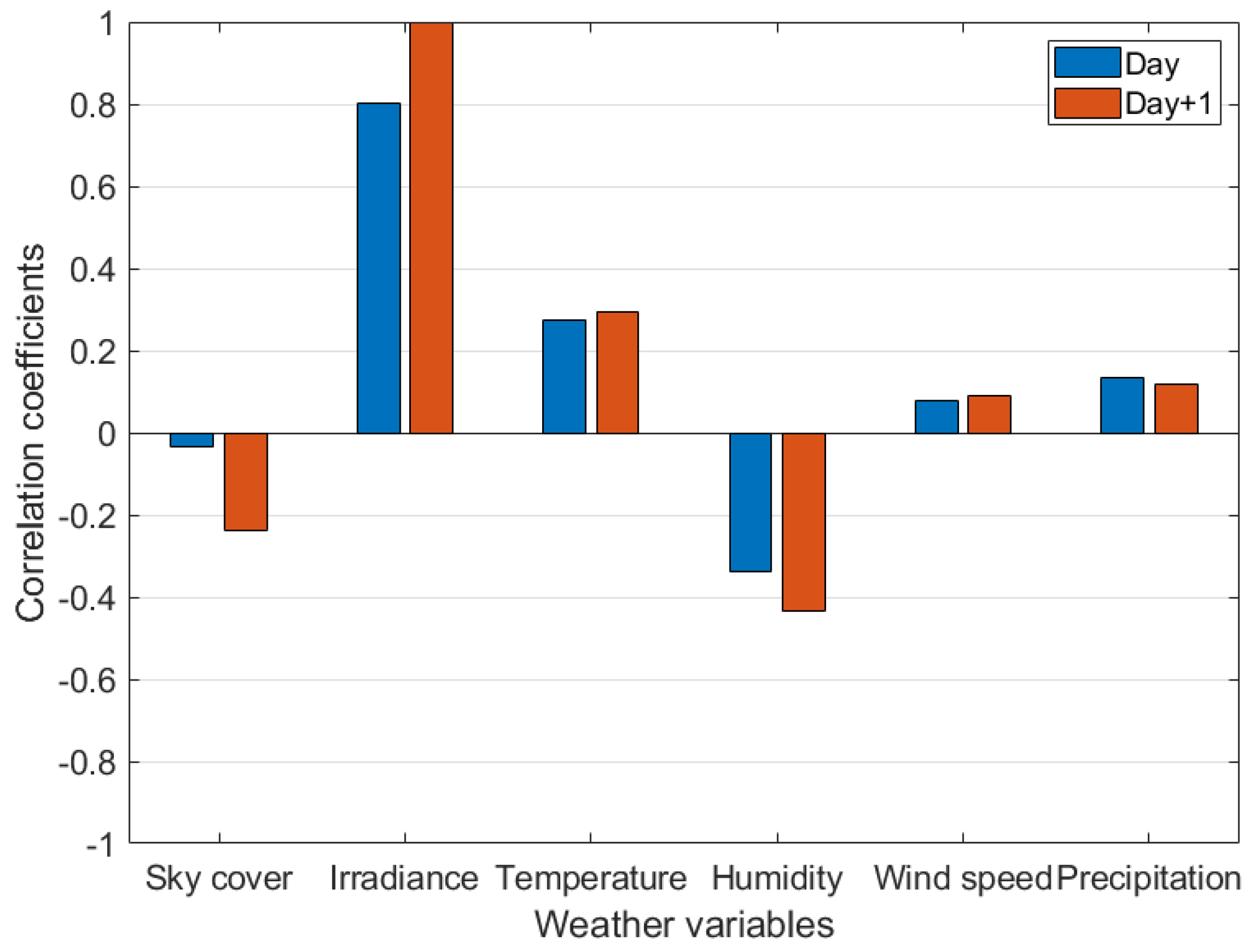
Figure 2 shows the results of analyzing the Pearson correlation between weather parameters and solar irradiance, and the data used for the correlation analysis are the annual weather data from five regions used to learn the proposed model. That is, the data used in the sample are 1825 days (365 × 5). The correlation ranges between −1 and 1, and it can be interpreted that the closer to 1 or −1, the higher the correlation with the solar irradiance pattern of the next day, and the closer to 0, the lower the correlation. As the results show, the solar irradiance of the previous day (Day) was 0.8, indicating that it was very highly correlated with the solar irradiance of the following day. Most weather parameters except sky cover were very similar in the Day and Day + 1 cases, indicating that they had very similar correlations. Furthermore, it was confirmed that the precipitation of the previous day was slightly more related than that of the following day to the pattern of solar irradiance on the following day.
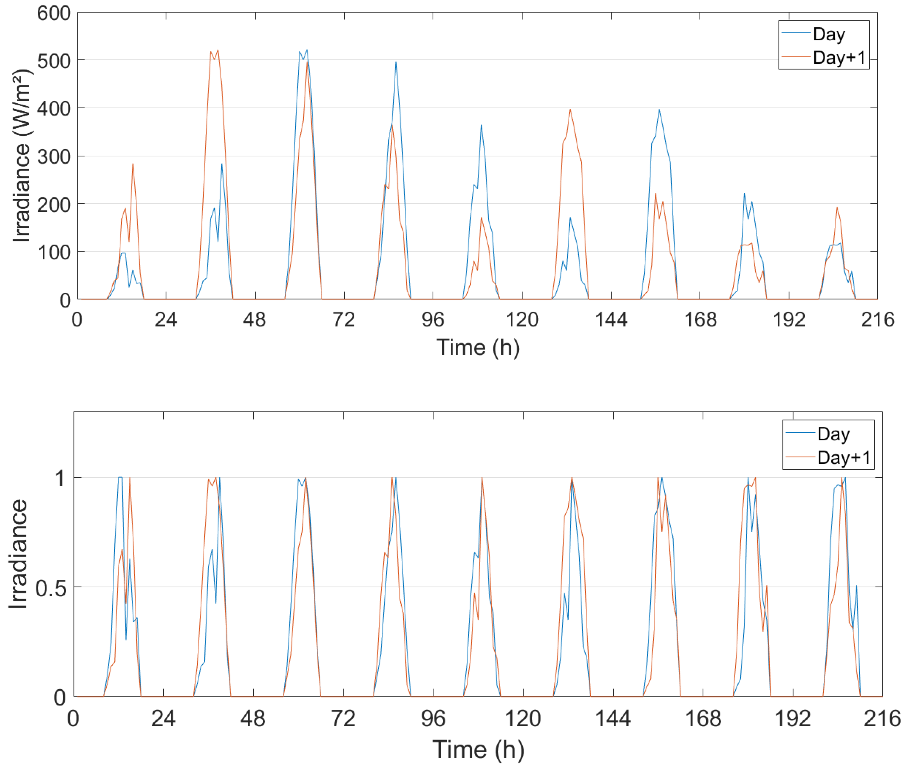
Figure 3 shows the pattern of solar irradiance during January 1–9 in Incheon, used for testing purposes. In the upper graph, solar irradiance exhibits a large deviation from that of the previous day; however, as shown in the graph below, assuming that the point at which the maximum solar irradiance occurs during the day is 1, the normalization of values maintains the width and height of the graph, enabling the isolation of the solar irradiance pattern. Thus, the data of solar irradiance on the previous day can be included. Normalization is a critical process in learning because these characteristics highlight how regional patterns of solar irradiance and time zones with different solar irradiance can be used.
Therefore, in the proposed model, the weather information of the previous day (Day), including solar irradiance, was used for learning, in addition to the input value used in the reference model. In the proposed solar irradiance model, once learning proceeded, only the weather information of the next day was updated under the assumption that data transmission is possible every 24 h only in the use stage. The weather region used for learning and testing in the model was the same as that in the reference model. Table 2 summarizes the relationship between the input data and output data of the reference model and the proposed model.
The weather data used in this study were TMY2 data provided by TRNSYS, an energy analysis program. TMY2 provides various types of weather information; however, the purpose of this study was to predict the amount of solar irradiance using limited forecast data provided by the weather forecast system. Therefore, only the forecast information (outdoor air temperature, humidity, wind speed, and precipitation information) obtained from the weather forecast system of Korea, a test region, was collected (Figure 4). In addition, hourly data can be secured in TMY2. As shown in Table 2 and Figure 4, meteorological parameters excluding precipitation are forecasted every 3 h on the previous day, and hourly solar irradiance information is required to apply to MPC. Therefore, an average of the TMY2 data was calculated at 3 h intervals to generate similar forecast data and regenerate hourly data through linear interpolation. For precipitation, hourly data were regenerated in the same manner, considering the forecast interval of 6 h. In addition, Korea’s cloud forecast categories are of four types (mostly cloudy, cloudy, partly cloudy, and clear sky), which are simpler than those of TMY2, which expresses sky cover with values between 0 and 100. Therefore, the sky cover data of TMY2 were also simplified to four types at 25% intervals, as in Korea’s weather forecast system. Because the purpose of this test was to verify the performance of the model using existing data and compare the performance of the models, it was assumed that the weather forecast would accurately predict the TMY2 data.
2.2.3. Proposed Model with Global Data
In the case of the proposed model, major domestic cities with relatively similar weather conditions were used as learning data. We evaluated the model performance by using different country data with less similar weather patterns. We referred to the proposed (global) model, and the same weather parameters were used; however, solar irradiance and weather information from different countries were used for model learning. The regions used for the prediction model were Cape Town, Canberra, Colorado, and Paris, and solar irradiance data for each region were selected. We used the notations and their definitions used in Koppen–Geiger, a representative climate classification method [46]. The climates can be classified in the order of main climate, seasonal precipitation type, and heat level. According to the classification criteria, Korean cities, which are used as input data for the test region and proposed model in this study, exhibited similar climatic conditions (Snow/Fully-humid/Hot-summer vs. Snow/Winter/Hot-summer), and the climates of the cities that were used as the input to the proposed (global) model were not the same as that of Incheon, the test region. The classification of regions, latitude, longitude, and Koppen–Geiger used in the proposed model and the proposed (global) model in this study are summarized in Table 3.
Considering the general characteristics of a deep learning model in which the performance of the model improves as more data are available for learning, if the proposed (global) model shows successful results in predictive performance, the available data from different climate zones can be used for learning; thus, this method can be useful when data in the local and surrounding regions are insufficient.
Figure 5 presents the input/output vector of the reference model that was compared with the proposed model or the proposed (global) model. Weather information of Day and Day + 1 predicted by the Meteorological Agency was largely used, and in the case of solar irradiance, the field measurement value of the target region was connected as an input vector. Then, the optimal weight and bias for deriving next-day solar irradiance was learned. All input values were interpolated and normalized according to time. In particular, the maximum solar irradiance and sunshine duration for the next day was affected by the present day’s solar irradiance and duration with other input conditions; therefore, the same normalization was important for successive days. Thus, in the case of the proposed (global) model, even if the model has learned in a region with a different climate, the field value for the present day is used for prediction. Thus, it is expected that there will be a correction effect in the prediction for other regions with different learning environments.
3. Simulation Results and Analysis
Under the assumption that data communication is performed on a daily basis, the input data of the model used for prediction was updated once every 24 h, and the model predicted with the update to establish the 24 h solar irradiance of the next day. Learning was the same as the prediction method using the model but aimed to correct the internal coefficient in the direction where the prediction error was minimized. The predicted results of the model were evaluated using the root mean square error (RMSE) and coefficient of variation of the RMSE (CVRMSE) [47], which are general error evaluation methods, as shown in Equations (8) and (9).
Here, is the measured value for time t, TMY2 data, and denotes the predicted value.
3.1. Comparison Between Reference and Proposed Model
First, the proposed LSTM prediction model and the reference model were constructed through the connection strength between neurons and layers that best described the relationship between the patterns of solar irradiance in the five regions. If the model similarly depicted the pattern of solar irradiance in the learning data of the five regions, it was expected that the error could be reduced in the prediction. Therefore, prior to the prediction, the learning performance of the model was analyzed, and the results are shown in Figure 6a. The learning error (RMSE) was 39.42 W/m2 for the reference model and 26.08 W/m2 for the proposed model. The scatter diagram indicates that more the points are distributed diagonally, the more accurate the model is. Most points were distributed around the diagonal line, but the learning performance of the proposed model was improved by approximately 22 W/m2 by utilizing more inputs to describe the target data. To increase the learning performance, the model can be enhanced by strengthening the hidden layer and the number of iterative learning; however, excessive learning performance settings may require significant time and a high-performance learning device or cause an over-fitting phenomenon. Figure 6b shows the performance results of predicting the solar irradiance in Incheon, the target region used for the reference model, and the proposed model showed a similar level of error in the learning performance.
As shown in Figure 6, the reference model using only forecast information showed RMSE of 50.89 W/m2 and CVRMSE of 36%. The proposed model, which additionally learns the weather pattern of the previous day, showed high predictive performance with an RMSE of 18 W/m2 and CVRMSE of 12.9%. Figure 7 shows the predictive performance comparison according to sky type. As shown in Figure 7, the reference model showed the highest error in mostly cloudy conditions with relatively little solar irradiance.
Figure 8 shows the predictive performance of each model at random intervals. As observed in the figure, the reference model is also excellent in the interval where the solar irradiance was relatively high, but the pattern of solar irradiance was not constant, and on the day when solar irradiance was relatively low, the reference model exhibits a large error. For example, the reference model showed the pattern of solar irradiance that failed to cope with sudden solar irradiance fluctuations, such as the 1057–1150 interval, where the change in solar irradiance over time is relatively large owing to sudden weather fluctuations and the pattern of solar irradiance with similar errors for four consecutive days.
As the proposed model learned more diverse time-series data patterns, including the weather conditions of the previous day, the model depicted patterns of solar irradiance similar to the actual one in all intervals. As mentioned earlier, it exhibited excellent predictive performance even when the solar irradiance during a day fluctuated suddenly. Figure 9 shows the predictive performance and weather conditions of each model in the interval of 1033–1153, where the error of the reference model was intensified.
As shown in Figure 9, all weather parameters, except sky cover, exhibited a considerably different pattern of occurrence from that in the previous day. That is, if the weather pattern of the previous day was added, as in the proposed model, it was possible to construct a more accurate solar irradiance prediction model even in the same type of learning parameter condition as the reference model.
The error of the proposed prediction model was a difference of 18 W/m2 on average. Based on the study by Jeon et al. [15], in which the error of horizontal solar irradiance of 79 W/m2 in the Energy Plus single residential building template generated a build load error of approximately 2%, it was determined that the proposed model can provide prediction values suitable for MPC control.
3.2. Proposed (Global) Model Results
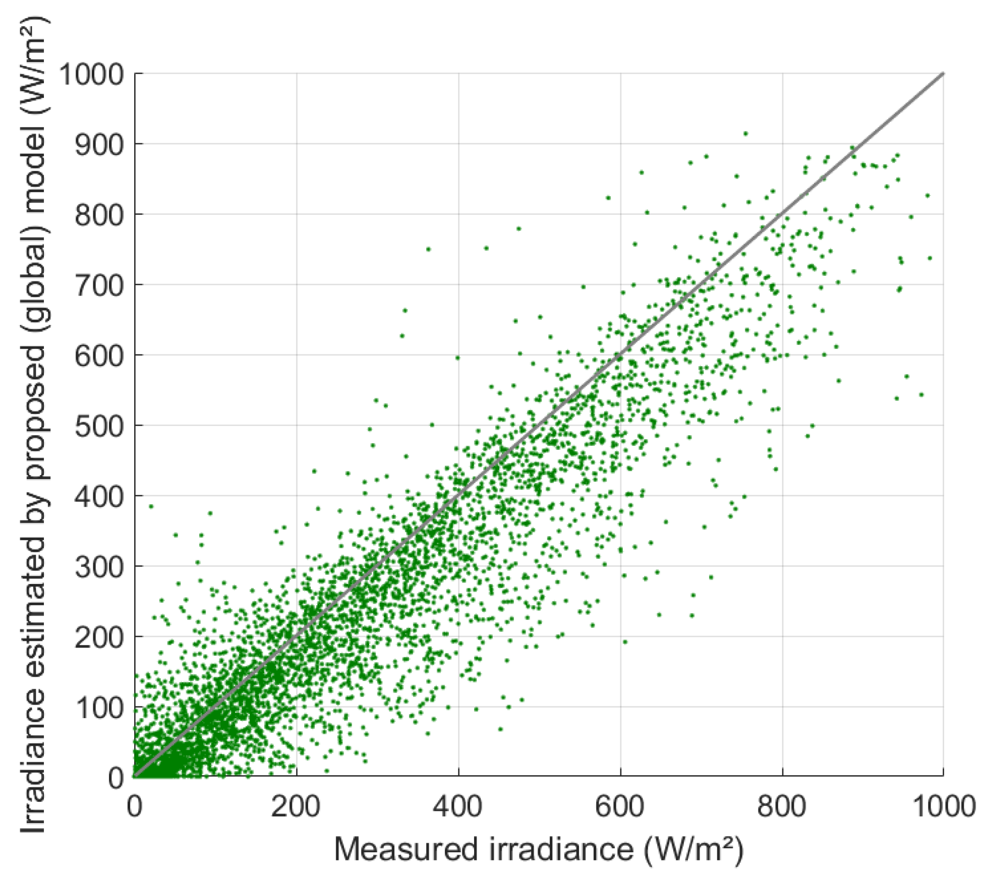
The proposed (global) data model is a model that learns using weather data from regions other than the prediction target city. Figure 10 shows the annual predictive performance of the proposed (global) data model. Overall, it was predicted to be less than the actual solar irradiance, but most points are distributed around the scatter diagram.
The model yielded an error of 15.9 W/m2 in the learning, and the learning performance of the model was similar to that of the proposed model, which learned the data of the region close to the target region. Figure 11 depicts the predictive performance of the proposed (global) model in random intervals. Even if the model has learned the solar irradiance data of completely different regions, it showed similarity in the pattern of the solar irradiance in most intervals with an error of 21.6 W/m2.
The learning and predictive performance of the various models proposed in this study are summarized in Table 4. The results of this study were excellent based on an RMSE of 76 W/m2, which was the prediction result in a previous similar study [33]. It should be noted that the models in majority of the existing studies are similar to the reference model in which the comparative experiment was conducted. However, because typical weather data were used in this study, weather prediction errors were not included.
4. Conclusions
In this study, an LSTM-based learning model was proposed to predict solar irradiance, which is the main input data required for the predictive control of buildings. The proposed model has the following three advantages over the existing solar irradiance prediction model. First, the proposed LSTM model uses data mostly provided by the weather forecasting system that can be easily obtained with the Application Programming Interface. Second, long-term measured data in the target region are not required for learning. As confirmed in previous studies, most models require long-term measured weather information in a region to predict local solar irradiance. Third, the proposed deep learning model does not require additional learning to update the model once it is constructed. Because the existing deep learning model for solar irradiance prediction uses data measured in a specific region, it is typical to update the model by periodically learning the measured data to improve model performance.
Owing to limitations such as the lack of measurement equipment and high cost in a small building or a building where MPC is newly applied, it is impossible to obtain historical data measured for several years. Moreover, a small CPU system installed for the MPC application cannot learn a substantial amount of data; therefore, continuous update is difficult. In this study, a model was developed that requires learning only once and can continuously predict the solar irradiance in a specific region using the existing solar irradiance data provided by other regions or other countries. Additionally, to improve the performance, a method for learning weather data from the previous day was proposed in this study, unlike the existing method that uses only the next day’s forecast information and the corresponding solar irradiance data.
The proposed model was verified by using the weather data of five among the six regions in Korea secured through TMY2 for learning and the solar irradiance data of the remaining region for prediction. The proposed model showed an RMSE of 17.4 W/m2 in the learning performance and 18 W/m2 in the predictive performance. According to previous studies, a model can be used for predictive control with a corresponding error of 2% or less when applied to a building load model. Through a method of learning the existing pattern of solar irradiance in other foreign countries, the proposed (global) model identified the patterns of solar irradiance fluctuations in a specific region that lacks accumulated data and provided reliable prediction results. The proposed learning model can exhibit excellent predictive performance with an RMSE of 30 W/m2 even when using intercontinental weather data far away from the prediction region; therefore, in practice, it can predict local solar irradiance using data from the region with a well-equipped database through long-term measurement. The verification result of the proposed model may have an increased error according to the forecast accuracy of the Korea Meteorological Administration; however, based on the fact that it predicted solar irradiance more accurately in the same test environment than did the reference model that was applied to the existing learning method, an improved predictive performance is expected in the future when this model is applied to the experimental environment of solar irradiance.
Author Contributions
All the authors developed and tested the presented models and methodologies; B.-k.J. drafted this manuscript; E.-J.K. revised it, and the other authors approved the current manuscript. All authors have read and agreed to the published version of the manuscript.
Funding
This work was supported by Korea Institute of Energy Technology Evaluation and Planning (KETEP) grant funded by the Korea government (MOTIE) (2019271010015D, Development of Smart city Energy Business Service)
Conflicts of Interest
The authors declare no conflict of interest.
Nomenclature
| weight matrices [-] in LSTM layer | |
| bias vector in LSTM layer | |
| candidate cell-state value in LSTM layer | |
| coefficient vector for outputs of the LSTM layer | |
| sigmoid function | |
| input vector at timestep t in LSTM layer | |
| measured solar irradiance over time t (W/m2) | |
| predicted solar irradiance over time t (W/m2) |
References
- Zhuang, J.; Chen, Y.; Chen, X. A new simplified modeling method for model predictive control in a medium-sized commercial building: A case study. Build. Environ. 2018, 127, 1–12. [Google Scholar] [CrossRef]
- Henze, G.P.; Felsmann, C.; Knabe, G. Evaluation of optimal control for active and passive building thermal storage. Int. J. Therm. Sci. 2004, 43, 173–183. [Google Scholar] [CrossRef]
- Lee, J.; Wang, W.; Harrou, F.; Sun, Y. Reliable solar irradiance prediction using ensemble learning-based models: A comparative study. Energy Convers. Manag. 2020, 208, 112582. [Google Scholar] [CrossRef] [Green Version]
- Dong, N.; Chang, J.F.; Wu, A.G.; Gao, Z.K. A novel convolutional neural network framework based solar irradiance prediction method. Int. J. Electr. Power Energy Syst. 2020, 114, 105411. [Google Scholar] [CrossRef]
- Ferreira, P.M.; Ruano, A.E.; Silva, S.; Conceicao, E.Z.E. Neural networks based predictive control for thermal comfort and energy savings in public buildings. Energy Build. 2012, 55, 238–251. [Google Scholar] [CrossRef] [Green Version]
- Huang, H.; Chen, L.; Hu, E. A new model predictive control scheme for energy and cost savings in commercial buildings: An airport terminal building case study. Build. Environ. 2015, 89, 203–216. [Google Scholar] [CrossRef]
- Kusiak, A.; Li, M.; Tang, F. Modeling and optimization of HVAC energy consumption. Appl. Energy 2010, 87, 3092–3102. [Google Scholar] [CrossRef]
- Nguyen, T.T.; Yoo, H.J.; Kim, H.M. Analyzing the impacts of system parameters on MPC-based frequency control for a stand-alone microgrid. Energies 2017, 10, 417. [Google Scholar] [CrossRef] [Green Version]
- Afram, A.; Janabi-Sharifi, F. Theory and applications of HVAC control systems–A review of model predictive control (MPC). Build. Environ. 2014, 72, 343–355. [Google Scholar] [CrossRef]
- Khanmirza, E.; Esmaeilzadeh, A.; Markazi, A.H.D. Predictive control of a building hybrid heating system for energy cost reduction. Appl. Soft Comput. 2016, 46, 407–423. [Google Scholar] [CrossRef]
- Korea Meteorological Administration. Available online: https://www.weather.go.kr/ (accessed on 9 October 2020).
- National Meteorological Service for the UK. Available online: https://www.metoffice.gov.uk/ (accessed on 9 October 2020).
- The National Weather Service U.S. Available online: https://www.weather.gov/ (accessed on 9 October 2020).
- National Meteorological Service for Canada. Available online: https://weather.gc.ca/ (accessed on 9 October 2020).
- Jeon, B.K.; Kim, E.J.; Shin, Y.; Lee, K.H. Learning-based predictive building energy model using weather forecasts for optimal control of domestic energy systems. Sustainability 2019, 11, 147. [Google Scholar] [CrossRef] [Green Version]
- Aggarwal, S.K.; Saini, L.M. Solar energy prediction using linear and non-linear regularization models: A study on AMS (American Meteorological Society) 2013–14 Solar Energy Prediction Contest. Energy 2014, 78, 247–256. [Google Scholar] [CrossRef]
- Wang, F.; Mi, Z.; Su, S.; Zhao, H. Short-term solar irradiance forecasting model based on artificial neural network using statistical feature parameters. Energies 2012, 5, 1355–1370. [Google Scholar] [CrossRef] [Green Version]
- Black, J.N. The distribution of solar radiation over the earth’s surface. Archiv. für Meteorol. Geophys. Bioklimatol. Ser. B 1956, 7, 165–189. [Google Scholar] [CrossRef]
- Samimi, J. Estimation of height-dependent solar irradiation and application to the solar climate of Iran. Solar Energy 1994, 52, 401–409. [Google Scholar] [CrossRef]
- Paltridge, G.W.; Proctor, D. Monthly mean solar radiation statistics for Australia. Sol. Energy 1976, 18, 235–243. [Google Scholar] [CrossRef]
- Daneshyar, M. Solar radiation statistics for Iran. Sol. Energy 1978, 21. [Google Scholar] [CrossRef]
- Premalatha, N.; Valan Arasu, A. Prediction of solar radiation for solar systems by using ANN models with different back propagation algorithms. J. Appl. Res. Technol. 2016, 14, 206–214. [Google Scholar] [CrossRef] [Green Version]
- Vindel, J.M.; Polo, J.; Zarzalejo, L.F. Modeling monthly mean variation of the solar global irradiation. J. Atmos. Sol. Terr. Phys. 2015, 122, 108–118. [Google Scholar] [CrossRef]
- Lago, J.; De Ridder, F.; De Schutter, B. Forecasting spot electricity prices: Deep learning approaches and empirical comparison of traditional algorithms. Appl. Energy 2018, 221, 386–405. [Google Scholar] [CrossRef]
- Jiang, Y. Computation of monthly mean daily global solar radiation in China using artificial neural networks and comparison with other empirical models. Energy 2009, 34, 1276–1283. [Google Scholar] [CrossRef]
- Sharma, V.; Yang, D.; Walsh, W.; Reindl, T. Short term solar irradiance forecasting using a mixed wavelet neural network. Renew. Energy 2016, 90, 481–492. [Google Scholar] [CrossRef]
- Kemmoku, Y.; Orita, S.; Nakagawa, S.; Sakakibara, T. Daily insolation forecasting using a multi-stage neural network. Sol. Energy 1999, 66, 193–199. [Google Scholar] [CrossRef]
- Ahmad, A.; Anderson, T.N.; Lie, T.T. Hourly global solar irradiation forecasting for New Zealand. Sol. Energy 2015, 122, 1398–1408. [Google Scholar] [CrossRef] [Green Version]
- Benmouiza, K.; Cheknane, A. Forecasting hourly global solar radiation using hybrid k-means and nonlinear autoregressive neural network models. Energy Convers. Manag. 2013, 75, 561–569. [Google Scholar] [CrossRef]
- Linares-Rodríguez, A.; Ruiz-Arias, J.A.; Pozo-Vázquez, D.; Tovar-Pescador, J. Generation of synthetic daily global solar radiation data based on ERA-Interim reanalysis and artificial neural networks. Energy 2011, 36, 5356–5365. [Google Scholar] [CrossRef]
- Srivastava, S.; Lessmann, S. A comparative study of LSTM neural networks in forecasting day-ahead global horizontal irradiance with satellite data. Sol. Energy 2018, 162, 232–247. [Google Scholar] [CrossRef]
- Voyant, C.; Notton, G.; Kalogirou, S.; Nivet, M.L.; Paoli, C.; Motte, F.; Fouilloy, A. Machine learning methods for solar radiation forecasting: A review. Renew. Energy 2017, 105, 569–582. [Google Scholar] [CrossRef]
- Qing, X.; Niu, Y. Hourly day-ahead solar irradiance prediction using weather forecasts by LSTM. Energy 2018, 148, 461–468. [Google Scholar] [CrossRef]
- Lee, L.J. A study on fundamental and application of CNN and RNN. Broadcast. Media Mag. 2017, 22, 87–95. [Google Scholar]
- Cortez, B.; Carrera, B.; Kim, Y.J.; Jung, J.Y. An architecture for emergency event prediction using LSTM recurrent neural networks. Exp. Syst. Appl. 2018, 97, 315–324. [Google Scholar] [CrossRef]
- Hochreiter, S.; Schmidhuber, J. Long short-term memory. Neural Comput. 1997, 9, 1735–1780. [Google Scholar] [CrossRef] [PubMed]
- Graves, A.; Mohamed, A.R.; Hinton, G. Speech recognition with deep recurrent neural networks. In 2013 IEEE International Conference on Acoustics, Speech and Signal Processing; IEEE: Piscataway, NJ, USA, 2013; pp. 6645–6649. [Google Scholar]
- Fischer, T.; Krauss, C. Deep learning with long short-term memory networks for financial market predictions. Eur. J. Oper. Res. 2018, 270, 654–669. [Google Scholar] [CrossRef] [Green Version]
- Salman, A.G.; Heryadi, Y.; Abdurahman, E.; Suparta, W. Single layer & multi-layer long short-term memory (LSTM) model with intermediate variables for weather forecasting. Proc. Comput. Sci. 2018, 135, 89–98. [Google Scholar]
- Yazan, E.; Talu, M.F. Comparison of the stochastic gradient descent based optimization techniques. In 2017 International Artificial Intelligence and Data Processing Symposium (IDAP); IEEE: Piscataway, NJ, USA, 2017; pp. 1–5. [Google Scholar]
- Kingma, D.P.; Ba, J. Adam: A method for stochastic optimization. arXiv 2014, arXiv:1412.6980. [Google Scholar]
- Huang, P.; Wen, C.; Fu, L.; Peng, Q.; Tang, Y. A deep learning approach for multi-attribute data: A study of train delay prediction in railway systems. Inf. Sci. 2020, 516, 234–253. [Google Scholar] [CrossRef]
- Abhishek, K.; Singh, M.P.; Ghosh, S.; Anand, A. Weather forecasting model using artificial neural network. Proc. Technol. 2012, 4, 311–318. [Google Scholar] [CrossRef] [Green Version]
- MathWorks Inc. MATLAB Documentation, MathWorks; MathWorks Inc.: Natick, MA, USA, 2018. [Google Scholar]
- Jeon, B.K.; Lee, K.H.; Kim, E.J. Development of a Prediction Model of Solar Irradiances Using LSTM for Use in Building Predictive Control. J. Korean Sol. Energy Soc. 2019, 39, 41–52. [Google Scholar]
- Kottek, M.; Grieser, J.; Beck, C.; Rudolf, B.; Rubel, F. World map of the Köppen-Geiger climate classification updated. Meteorol. Z. 2006, 15, 259–263. [Google Scholar] [CrossRef]
- Ćalasan, M.; Aleem, S.H.A.; Zobaa, A.F. On the root mean square error (RMSE) calculation for parameter estimation of photovoltaic models: A novel exact analytical solution based on Lambert W function. Energy Convers. Manag. 2020, 210, 112716. [Google Scholar] [CrossRef]
Figure 1.
Structure of long short-term memory (LSTM) cell (reproduced from Graves [37]).
Figure 1.
Structure of long short-term memory (LSTM) cell (reproduced from Graves [37]).

Figure 2.
Pearson correlation analysis of weather information and solar irradiance.

Figure 3.
Analysis of patterns of solar irradiance on the previous day and the next day.

Figure 4.
Example of a Korean weather forecast system (Korea Meteorological Administration [11]).
Figure 4.
Example of a Korean weather forecast system (Korea Meteorological Administration [11]).

Figure 5.
Input/output of proposed and reference models.

Figure 6.
Comparison between learning and predictive performance of LSTM model.

Figure 7.
Predictive performance comparison according to sky cover (Reference vs. Proposed).


Figure 8.
Solar irradiance predictive performance comparison in a random interval (Reference vs. Proposed).
Figure 8.
Solar irradiance predictive performance comparison in a random interval (Reference vs. Proposed).

Figure 9.
Analysis of weather conditions and solar irradiance predictive performance used as input values in the reference model error interval.
Figure 9.
Analysis of weather conditions and solar irradiance predictive performance used as input values in the reference model error interval.

Figure 10.
Analysis of solar irradiance prediction of proposed (global) model.

Figure 11.
Comparison of solar irradiance prediction by proposed and proposed (global) models.


Table 1.
Parameter setting of LSTM model.
| Parameter | Value | Parameter | Value |
|---|---|---|---|
| Optimization algorithm | Adam | Hidden layer | 3 |
| Initial learning rate | 0.001 | Hidden Unit | 300(×3) |
| Execution environment | GPU | Max Epochs | 200 |
Table 2.
Input/output data of LSTM model.
| Model | Input Parameters | Initial Time Interval (h) | Input Data Interval (h) | Output Parameters |
|---|---|---|---|---|
| Reference | Temperature day+1 | 3 | 1 | Hourly irradiance day+1 for next 24 h |
| Humidity day+1 | 3 | 1 | ||
| Wind speed day+1 | 3 | 1 | ||
| Sky cover day+1 | 3 | 1 | ||
| Precipitation day+1 | 6 | 1 | ||
| Proposed | Temperature day, day+1 | 3 | 1 | Hourly irradiance day+1 for next 24 h |
| Humidity day, day+1 | 3 | 1 | ||
| Wind speed day, day+1 | 3 | 1 | ||
| Sky cover day, day+1 | 3 | 1 | ||
| Precipitation day, day+1 | 6 | 1 | ||
| Irradiance day | 1 | 1 |
Table 3.
Comparison of geographical characteristics of learning data of proposed model.
| Case | City | Nation | Latitude | Longitude | Koppen–Geiger Classification (Climate/Precipitation/Temperature) |
|---|---|---|---|---|---|
| Proposed | Kangnung | Asia/KOR | 37.7 | 128.8 | Snow/Fully-Humid/Hot-Summer |
| Kwangju | Asia/KOR | 35.1 | 126.7 | Snow/Fully-Humid/Hot-Summer | |
| Mokpo | Asia/KOR | 34.7 | 126.4 | Snow/Fully-Humid/Hot-Summer | |
| Seoul | Asia/KOR | 37.5 | 126.8 | Snow/Winter/Hot-Summer | |
| Ulsan | Asia/KOR | 35.5 | 129.2 | Snow/Fully-Humid/Hot-Summer | |
| Proposed (global) | Cape Town | Africa/ZAF | −33.9 | 18.4 | Arid/Steppe/Cold Area |
| Canberra | Oceania/AUS | −35.3 | 149.1 | Warm-Temperate/Fully-humid/ Warm-Summer | |
| Colorado | America/USA | 39.2 | −105.6 | Warm-Temperate/Fully-humid/ Hot-Summer | |
| Paris | Europe/FRA | 48.9 | 2.2 | Warm-Temperate/Fully-humid/ Hot-Summer | |
| Target | Inchon | Asia/KOR | 37.4 | 126.6 | Snow/Winter/Hot-summer |
Table 4.
Learning and predictive performance of LSTM model.
| Model | RMSE (W/m2) | CVRMSE (%) | |
|---|---|---|---|
| Ref. | Learning | 39.42 | 26.08 |
| Predictive | 50.89 | 36.48 | |
| Proposed | Learning | 17.48 | 11.56 |
| Predictive | 18.00 | 12.9 | |
| Proposed (global) | Learning | 15.93 | 9.04 |
| Predictive | 30.21 | 21.64 | |
© 2020 by the authors. Licensee MDPI, Basel, Switzerland. This article is an open access article distributed under the terms and conditions of the Creative Commons Attribution (CC BY) license (http://creativecommons.org/licenses/by/4.0/).
Share and Cite
MDPI and ACS Style
Jeon, B.-k.; Kim, E.-J. Next-Day Prediction of Hourly Solar Irradiance Using Local Weather Forecasts and LSTM Trained with Non-Local Data. Energies 2020, 13, 5258. https://0-doi-org.brum.beds.ac.uk/10.3390/en13205258
AMA Style
Jeon B-k, Kim E-J. Next-Day Prediction of Hourly Solar Irradiance Using Local Weather Forecasts and LSTM Trained with Non-Local Data. Energies. 2020; 13(20):5258. https://0-doi-org.brum.beds.ac.uk/10.3390/en13205258
Chicago/Turabian StyleJeon, Byung-ki, and Eui-Jong Kim. 2020. "Next-Day Prediction of Hourly Solar Irradiance Using Local Weather Forecasts and LSTM Trained with Non-Local Data" Energies 13, no. 20: 5258. https://0-doi-org.brum.beds.ac.uk/10.3390/en13205258
Note that from the first issue of 2016, this journal uses article numbers instead of page numbers. See further details here.