Viscosity Models for Drilling Fluids—Herschel-Bulkley Parameters and Their Use †


1
Department of Energy and Petroleum Engineering, University of Stavanger, N-4036 Stavanger, Norway
2
SINTEF Industry, S.P. Andersens vei 15 B, N-7031 Trondheim, Norway
*
Author to whom correspondence should be addressed.
†
This article is an extended version of the conference paper OMAE2019-96595, In Proceedings of the ASME 2019 38th International Conference on Ocean, Offshore and Arctic Engineering, 9–14 June 2019, Glasgow, Scotland.
Energies 2020, 13(20), 5271; https://0-doi-org.brum.beds.ac.uk/10.3390/en13205271
Submission received: 28 September 2020
/
Revised: 5 October 2020
/
Accepted: 9 October 2020
/
Published: 11 October 2020
(This article belongs to the Special Issue Advances in Drilling Fluid Technology)
Abstract
:An evaluation is presented of the practical usage of the Herschel-Bulkley viscosity model for drilling fluids. If data from automatic viscosity measurements exist, the parameters should be selected from relevant shear rate ranges to be applicable. To be able to be used properly, viscosity measurements must be measured with a sufficient accuracy. It is shown that a manual reading of standard viscometers may yield insufficient accuracy. It is also shown that the use of yield point/plastic viscosity (YP/PV) as measured using API or ISO standards normally provide inaccurate viscosity parameters. The use of the Herschel-Bulkley model using dimensionless shear rates is more suitable than the traditional way of writing this model when the scope is to compare different drilling fluids. This approach makes it also easier to make correlations with thermodynamic quantities like pressure and temperature or chemical or mineralogical compositions of the drilling fluid.
1. Introduction
The viscous properties of drilling fluids are measured for several purposes. Viscous data valid at some shear rates are needed to forecast annular frictional pressure losses during drilling. Low shear viscous data are needed to predict the stability of the drilling fluid with respect to the stability of drilling fluids like barite sag particle suspensions. High shear data, together with extensional performance is needed to predict the performance during flow through the drill bit. Other processes like filter loss and displacement efficiency may require data obtained at other shear rates. In the following documents current practical handling of such measurements and the consequences for parameter selection is outlined in accordance with Saasen and Ytrehus [1].
The current field applied drilling fluid viscosity measurement relies on measurement with a viscosity-gel meter (VG meter) made in accordance with standards like API [2] or ISO [3,4]. Even though the number of measurement points may be limited, these standards base their viscosity models on measurements conducted at a shear rate range typically spanning from 5.11 to 1022 1/s for drilling fluids and 5.11 to 511 1/s for well cement slurries [5], representing a span from 3 to 600 rpm on a VG meter. Earlier, the viscosity models were calculated based on viscosity measurements at shear rates of 511 and 1022 1/s, only. This practice is still relatively common in field operations. Hence, large viscosity errors are common in the evaluation of drilling fluid viscosity. In current standards, it is recommended to use a least square fit of all shear stress measurements, using their affiliated shear rates, to increase the accuracy of the viscosity models. Shear rates in excess of 250 1/s are seldom experienced for annular flow in the field [5,6,7], except for flow around the bottom hole assembly (BHA). Therefore, improved model accuracy can often be obtained if the least square fit is conducted only for the relevant shear rates of the drilling fluid flow situation. This improvement, however, requires a sufficient density of measurement points. A practical upper limit for the relevant shear rates for the Newtonian flow can be found using Equation (1). The wall shear rate for Newtonian flow is presented as 12 times the annulus velocity divided by the diameter difference. For typical drilling fluids being a shear thinning non-Newtonian fluid, this shear rate is somewhat larger. Equation (1) should be multiplied with a shear thinning correction factor. Equation (1) and the correction factor, Equation (2), are described in most textbooks about rheology or for example by Guillot [5]. The shear rate after this correction is shown in Equation (2). This correction factor, Equation (2), can be 2–3 for a 17 ½” section, but is seldom larger than 1.5 for an 8 ½” section. However, the Newtonian flow shear rate in a 17 ½” section is less than 30 1/s. Therefore, the actual shear rate in this section will be significantly smaller than that of the 8 ½” section. For the present study it is anticipated that the use of data applicable for the 8 ½” section also will be relevant for the larger sections as it has the highest typical annular shear rates. Hence, in the present article the shear rates up to 300 1/s was used as an example of the relevant shear rate regime. The shear rate for Newtonian flow in a concentric annulus can be found using Equation (1):
where v is the flow velocity in the annulus, do is the hole size and di is the drill pipe diameter.
The shear rate at the wall in an annulus is thus given as shown in Equation (2) (see for example Guillot [5]).
where the local power law index n’ is given as:
A large number of fluid models are used to describe complex fluid viscosities like those of drilling fluids. The range of these models include simple two-parameter models like the Bingham model to complex models trying to incorporate structure build-up and disruption like the Quemada model [8,9]. Cayeux and Leulseged [10] showed that the Herschel-Bulkley, Robertson–Stiff, Heinz–Casson and Carreau viscosity models fit better to drilling fluid viscosity measurement than the Bingham, Power Law or Newtonian fluid models do. Some researchers have also found that viscoelastic properties can be important when dealing with different drilling fluid engineering problems [6,11,12]. In addition, thixotropic effects may disturb the steady state viscometer reading for a relatively long time [13].
One relatively simple model describing the drilling fluid viscous flow curve with reasonable accuracy is the Herschel-Bulkley model. This model is named after Herschel and Bulkley [14], who described how such flow curves should behave. In the Herschel-Bulkley model the shear stress is related to a yield stress, τy, a consistency factor, k, and the shear rate, , in accordance with Equation (4).
The yield stress is the minimum shear stress applied to a material to create a flow. For any shear stress less than the yield stress, the material should ideally act as a solid material. The consistency factor, k, is dependent on the curvature exponent, n. Hence, k = k(n). The consequence of this dependency is that the consistency parameter cannot be determined directly from the fluid measurements. It must be identified through algebraic operations and, furthermore, it cannot alone contain information about physical dependencies for the fluid. An example of different combinations of k and n giving nearly similar flow curves is presented in Table 1, which show the values obtained if the parameters are determined by curve fitting using different ranges in shear rates from the same data set.
The values are Herschel-Bulkley parameters determined by least square fit of rheometer data after the determination of the yield stress. The numerical values of the consistency parameter developed by fitting measurements values from the shear rate range up to 300 1/s is less than half of the value obtained if all the measurement values up to 1000 1/s were used in the fit. This is an example of the fact that k cannot be used alone as a fluid property parameter. Its numerical value will always be dependent on the curvature index, n. Hence, tabulating the parameter k for other perspectives than reproducing numerical calculations is irrelevant.
Nelson and Ewoldt [15] presented a modified Herschel-Bulkley model with the scope of overcoming the limitations appearing when using the k and n approach. In their model, the Herschel-Bulkley model was rewritten as shown in Equation (5),
where . is the shear rate where the stress is equal to twice the yield stress. This model is intended primarily for measurement of 3D printing materials. One of their scopes was to tabulate material properties in such a way that the 3D print operator easily could select the applicable material. The principle introduced by Nelson and Ewoldt [15] is adequate for 3D printing. However, this specific method is not sufficiently practical for describing drilling fluids as measured in accordance with the API or ISO specifications. The main reasons for this are mainly threefold. First, the yield stress of a drilling fluid is normally very small or even absent. It is often difficult or sometimes impossible to present the shear rate where the shear stress is twice the yield stress. Second, the determination of the yield stress with sufficient accuracy at field locations is a challenge in itself, and, third, the number of measurement points and the accuracy of field viscometers are too limited to be of practical application to determine this parameter. Therefore, Saasen and Ytrehus [16] modified the model of Nelson and Ewoldt with respect to well fluid applications and presented the Herschel-Bulkley model with dimensionless shear rates as shown in Equation (6),
where the surplus stress, τs = τ − τy is determined at a relevant shear rate of . The surplus stress is not dependent on the curvature index, n, and can therefore be tabulated to represent a material property. An equally good, or sometimes better parameter to be tabulated is the measured shear stress at this relevant shear rate since this parameter directly correlates to the viscosity of that shear rate.
The measurement data shown in Table 1 was obtained with an Anton Paar Physica MCR 102 rheometer. The surplus stress, τs = 4.55 Pa, was measured at the shear rate of 201 1/s and the flow index, or the curvature exponent, n = 0.8107, at 101 1/s. These values represent a consistency factor equal to 0.0618 Pa·s−n. The results of frictional pressure loss calculations using the Founargiotakis [17] model show that measurements fitted to the Herschel-Bulkley model give a better approximation to the measured pressure loss if the data is collected from the relevant shear rate region [18]. This is shown in Figure 1 as the stippled line approaches the measured points better than the dotted line. It can also be seen that similar good results were obtained at the lowest shear rates if the model based on dimensionless shear rates was applied, as the solid line show the same results as the dotted line for the smaller shear rates. This is likely to be caused by having a good fit to the actual viscous data within this smaller shear rate range that were produced by the flow as the surplus stress shear rate was selected to be relevant for the flow situation.
For completeness, it is useful to explain the measurements shown in Figure 1 more thoroughly. The measurements at the two lowest velocities were conducted while the flow was laminar. For the higher flow rates, the flow gradually become more and more unstable for finally becoming turbulent as the flow rate increases. It should be noted that the measurements shown in Figure 1 are conducted for flow in a cased hole. Ytrehus et al. [19] has shown that the frictional pressure losses generally become higher in open hole sections compared to that of flow in the cased hole sections. A change from cased hole to open hole sections during flow in laminar flow conditions have lesser differences on the frictional pressure losses.
In current drilling fluid laboratories, it is industry practice to apply viscometers with at least six speeds. Still, most of these viscometers have visual readings. Hence, to evaluate the possibility of using data from such measurements in determination of Herschel-Bulkley parameters, eight measurement curves from a commercial laboratory will be evaluated. None of these measurements were conducted with the scope of being tested for detailed analysis of rheological parameters. The scope of the measurements was to provide operators with the flow curve. In the following sections, these measurements values will be used to evaluate the applicability of using the Herschel-Bulkley parameters in hydraulic analyses. Using this data set give the possibility of presenting typical examples of practical viscosity measurements of field fluids.
2. Viscosity Measurements
Currently there are many types of rheometers on the market. The more scientific apparatuses are very accurate but are not generally suitable for oilfield application. In field operations within the drilling industry equipment that are simple to use as no special trained operators may be available on site is needed. Furthermore, the equipment needs to be of a type that will tolerate movement. Finally, the equipment must be of a type that can be applied to different fluids with different particle contents. Particles in the drilling fluids may exceed 100 microns. Hence, if a concentric cylinder device is used as recommended by oilfield standards [2,3,4], the annular gap should be larger than 1 mm. In oilfield equipment following these standards, the outer viscometer radius, R2, is 18.415 mm and the inner radius, R1, is 17.247 mm. This leaves a concentric cylinder annular gap equal to 1.168 mm. As will be shown in the following discussion, construction of equipment in accordance with these requirements limits the accuracy of standard equipment.
Suitable instrumentation for viscosity measurements is described by for example Guillot [5] who concentrated on well cement measurements and Mezger [20] who presented general viscometer technology. Concentric cylinder devices are normally applied for the measurement of drilling fluid viscosity. The most common field instrumentation is 6 speed VG viscometers [2,3,4]. With these instruments it is not possible to measure the flow curve within the most important shear rate range for field application. During the last decades it has also become common with at least two more shear rates in field instruments. A conversion between VG meter RPM, as applied in accordance with API and ISO specifications [2,3,4], and shear rates in 1/s is given by RPM × 1.703 = 1/s.
Most equipment built in accordance with oil field specifications [2,3,4] are manually operated. A consequence of this is the introduction of measurement errors that are not systematic. From practical experience, it is assumed that the shear stress read out error is around ± one dial reading, introducing an extra uncertainty for measurements at 102.2 1/s or less. One dial reading is a stress equal to one lbf/100 ft2, or 0.511 Pa in SI units. In the following analysis a selection of shear stress measurement data from eight arbitrary drilling fluid samples is used as examples to explain the consequences for drilling fluid viscosity determination. The fluids are all field applied drilling fluids or fluids made for field application. All fluids are either measured on the rig site or in the drilling fluid laboratory. For most of the curves there are a couple of measurement points most likely being incorrect by a couple of dial readings. These inaccuracies are visible primarily for shear rates less than 340.7 1/s, since an error of dial reading is less important at measurements at the two highest shear rates. A conclusion is that the drilling fluid engineer measuring the drilling fluid viscosity must have full attention to correctly measure and register the shear stresses at all shear rates. In addition, as being described by for example Guillot [5], along with the curvature, the large gap between the viscometer bob and cylinder will bring in an uncertainty about the correct shear rate. For the smaller shear rates this uncertainty can be as large as 20% [5]. Another uncertainty that is described in most textbooks on slurry rheology, for example Whorlow [21], arises since the torque is constant as a function of the radius in the viscometer. In the presence of a yield stress the shear stress at the outer viscometer cylinder may be less than this yield stress for the smallest shear rates. The reduction in shear stress at the outer cylinder compared to the inner cylinder is equal to (R1/R2)2. Using the standard dimensions [2,3,4] presented earlier, this value is 88%. Hence, if the minimum shear stress at the lowest shear rates is only 14% larger than the yield stress, the fluid in the near vicinity of the outer cylinder will be less than the yield stress and not deformed continuously, leading to an unknown shear rate in this measurement.
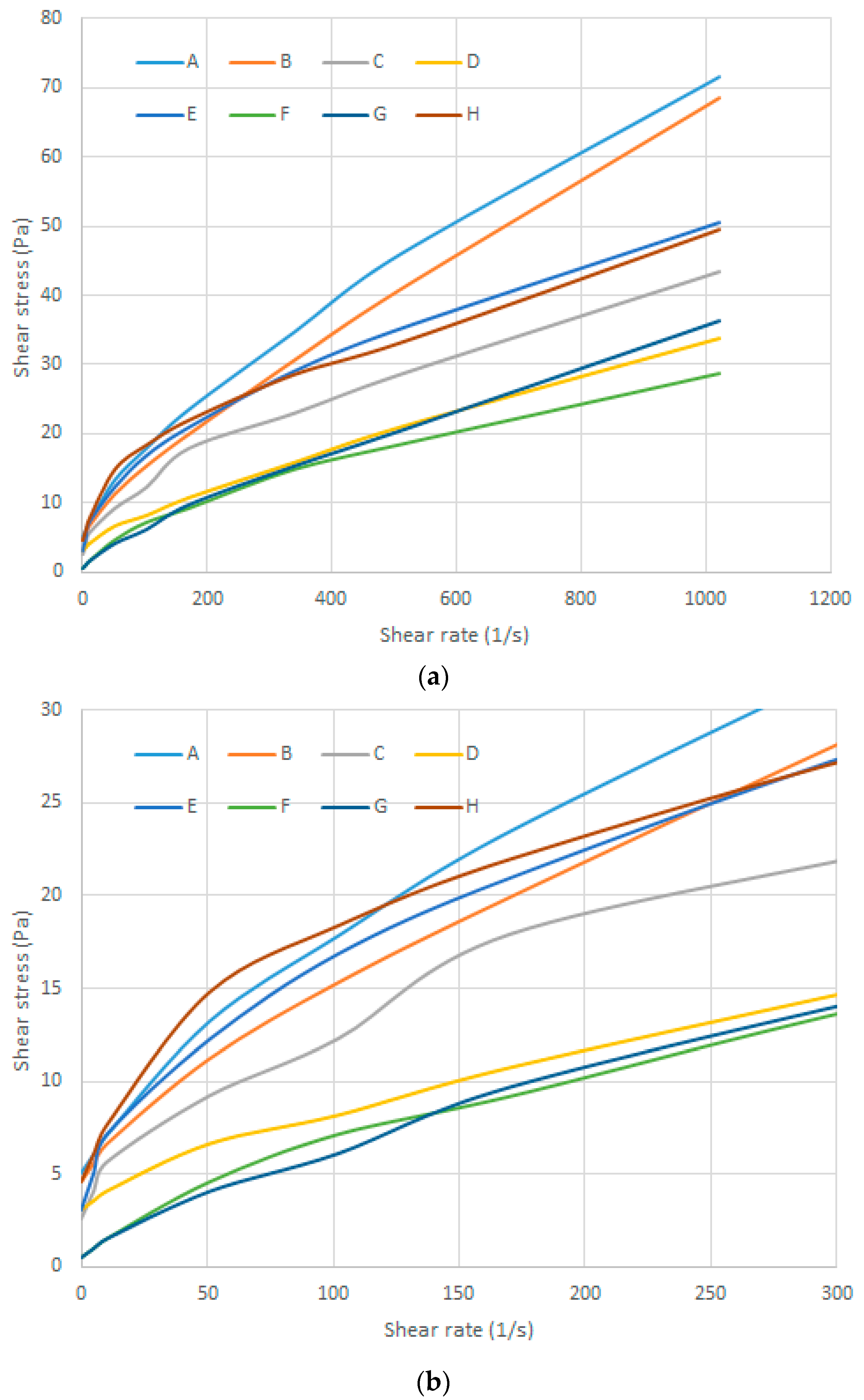
When the measurements are conducted with automatic high accuracy instruments, as in the data used in Table 1, it is shown the importance of using data from the correct shear rate range in developing the viscosity model for the drilling fluid. The data shown in Figure 2 are examples measured at drilling fluid laboratories. As presented earlier, none of these measurements were conducted with the scope of being tested for detailed analysis of rheological parameters. The scope of the measurements was simply to provide operators with the flow curve for technical discussions. Hence these data are perfect examples on how the manually registered viscometer data appears. It can be observed in the measurements at shear rates less than 300 1/s that the slope of some of the curves suddenly increases and then decreases again. These fluids are all typical field fluids from the North Sea area. If measured properly, these fluids will have a monotonic variation of the slope. Hence, there are inaccuracies in the recorded data for these fluids. When inaccuracies appear at the relevant shear rate data as being the case for the fluids shown in Figure 2, the average error for all the fluids seems to be relatively equal if the Herschel-Bulkley parameters are based on all the measurements or the measurements at the relevant shear rates. Thus, it is imperative to have full attention to obtain accurate shear stress measurements at all shear rates if the measurements are to be used for determination of Herschel-Bulkley parameters. This is especially important for measurements at shear rates in the relevant shear rate range for annulus flow, since an error of one dial reading becomes more significant the lower the shear stress becomes.
3. The Yield Stress
For the last decades after Barnes and Walters [22] claimed that a yield stress does not exist, it has been a large discussion about the reality of a yield stress [23,24,25]. Mezger [20] concludes that a yield stress cannot be a flow property since its value is dependent on the low shear rate resolution and the ramp up or ramp down time of the flow curve. Professor Phil Banfill mentioned in a presentation at the International Conference on Rheology of Fresh Cement and Concrete, in Liverpool (26–29 March 1990) that by the time required to prove non-existence of a yield stress for solidifying fluids, the fluid would have solidified. Another beautiful treatment of the yield stress problem was given by Niall Young and Mats Larsson at the Nordic Rheology Conference in Tórshavn, the Faroe Islands in 2003. They enacted a play where they acted as Sherlock Holmes and Dr. Watson [26] discussing the diabolical case of the recurring yield stress. They ended with a conclusion parallel to one of the most accepted statements about the yield stress that was given by Astartia [23]: “Whether yield stress is or is not an engineering reality depends on what problem we are considering, not on how long a ball appears to be standing still”. His view seems to be supported by Evans [24]. Thus, for the short time scales present in drilling, stresses below a yield stress will only present an elastic deformation without flow. The fluid will flow only in the presence of shear stresses above the yield stress. Hence, for the application of the fluid, the yield stress is a material property describing the start-up of flow of complex materials within drilling engineering. The drilling fluid yield stress will depend on the fluid composition. The yield stress value will change dependent on several fluid composition parameters including solid fraction and emulsified particles of a certain size in the fluid and concentration of different polymers as well as the presence of surface-active chemicals.
Determination of the drilling fluid yield stress is a challenge. The original rotational viscometer developed more than half a century ago was a two speed instrument. The shear rates and dimensions were designed to be accurate within that day’s practical technology limits. Hence, both the yield stress and a plastic viscosity were measured using this device. As will be shown in the next paragraphs, this yield point/plastic viscosity (YP/PV) concept as being described in standards [2,3,4] is inadequate to approximate both the yield stress and the viscosity at lower shear rates [10]. The plastic viscosity is determined from a linear fit of the viscosity measurements at the shear rates 511 and 1022 1/s, and by extrapolation to the zero shear rate the yield point is determined.
Several concepts are used to determine the yield stress. These range from the maximum stress where viscoelastic properties are able to stay within the linear range to simple approximations like the low shear yield stress developed by Zamora and Power [27], who approximated the yield stress with a linear extrapolation from the two lowest shear rates of the viscosity-gel (VG) meter. Probably the low shear yield stress will predict a yield stress some percent higher than the best approximation possible using the standard oil field equipment. The analysis of the current data shows that the yield stress may be around 90% of the predicted value from Zamora and Power [27]. However, no systematic adjustments to their values have yet been found. This seems to be in line with findings by Power and Zamora [28] who evaluated the yield stress approximated following Zamora and Power [27]. They based their study on statistical analysis of measurements on a huge number of drilling fluids. They concluded that the approximation is reasonably accurate. This conclusion seems to be adequate, following the discussion in previous paragraphs, as the shear rates obtained at the inner cylinder can deviate significantly from the anticipated shear rate for the low rpm readings of the VG-meter [29]. Hence, most ways to improve the accuracy directly without using iterative algorithms seem doubtful.
Present industry specifications are designed to be used for 6 speed VG-meters. Many instruments made in accordance with these specifications do not cover the relevant viscosity range sufficiently. Hence, it is desirable to also measure some viscosity values between the shear rates of 10.22 1/s and 170.3 1/s (6 and 100 rpm). In Figure 3 it is shown the viscosity error, being the calculated viscosity divided by the measured viscosity, where the drilling fluid viscosities are modelled as Bingham fluids using YP and PV calculated in accordance with API/ISO specifications [2,3,4]. The viscosity is modelled with large errors in the relevant shear rate ranges for the annulus flow of drilling fluid. The yield stress is normally approximated to be several hundred percent larger than the yield stress determined following the procedures suggested by Zamora and Power [27].
4. The Surplus Stress or Consistency Factor and the Flow Behaviour Index
The Herschel-Bulkley model uses a yield stress onto which a term consisting of a consistency multiplied with a flow behaviour index is added. The flow behaviour index is in reality a curvature index for fluid behaviour at non-zero shear rates. The accuracy of the model, especially at lower shear rates depends on the suitability of the method chosen to approximate the yield stress. If it is not properly determined the high shear rate deviations from measurement points may not be significant. However, as described earlier, the shear stresses at these high shear rates are mostly relevant for the flow inside the drill string and around the drill string’s BHA.
When the actual shear rate range for the flow problem is defined it is necessary to select two typical shear rates from this range. These shear rates should include a characteristic high shear rate and a characteristic low shear rate for the flow problem. The surplus stress should be selected at one of these shear rates and the curvature exponent should be selected at the other. In the following examples the surplus stress, τs, will be calculated for the measurement at 170.3 1/s (100 RPM) and the flow behaviour index, or more correctly, the curvature exponent, will be calculated at 102.2 1/s (60 RPM). Hence these data will be mostly relevant for flow in an 8 ½” (216 mm) section.
It is seen from the data shown in Figure 2 that several of the flow curves had a slope that is non-monotonic as a function of the shear rate. Most likely, there are erroneous measurements at some shear rates for fluids C, D, G and H, as their flow curves demonstrate such non-monotonic slopes. As the remaining flow curves all have a slope that is monotonic with a shear rate, it is assumed that these are more accurately measured. The viscosity measurement of these remaining fluids, fluids A, B, E and F, are used to compare the Herschel-Bulkley model with parameters determined in accordance with API or ISO specifications (labelled “old”) and with the Herschel-Bulkley model used with direct measurements at two relevant shear rates (labelled “New”).
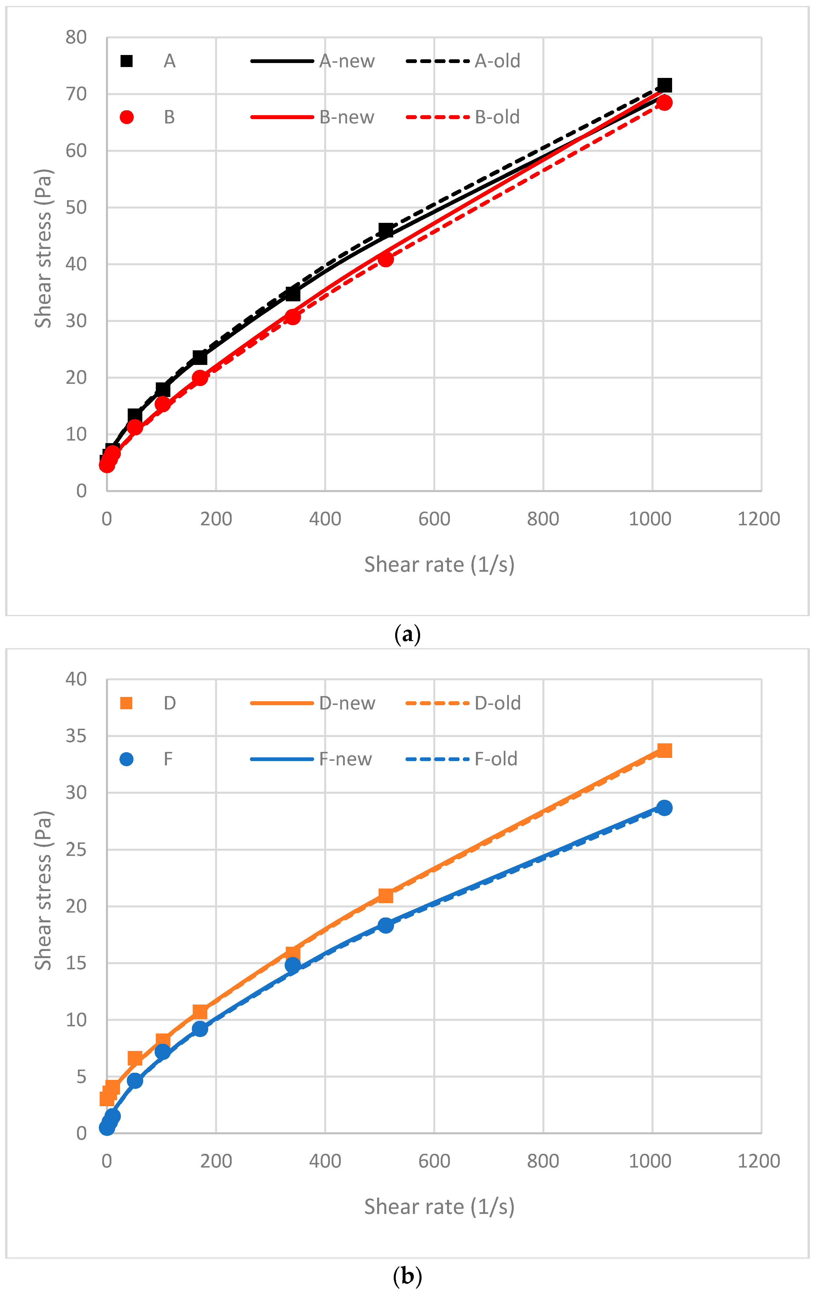
In Figure 4 it is shown the flow curves for the drilling fluids A and B. The solid line represents the fluids modelled with Herschel-Bulkley parameters determined directly from viscometer measurements at two relevant shear rates, while for the stippled line these parameters are determined in accordance with oilfield specifications [2,3,4]. Most likely, the fluid A is indeed a Herschel-Bulkley fluid. As can be seen from comparing the curves for this fluid in Figure 4, it is irrelevant, which method has been used to determine the model parameters. The measurements are predicted within reasonable accuracy anyhow. The viscosity curve of Fluid B seems to have a different behaviour than Fluid A. The standard calculations underestimate the viscosity at lower shear rates. At the two highest shear rates the traditional calculation must predict the shear stress as these numbers were used to calculate the model parameters. Similarly, for the dimensionless shear rate model, this model is forced to predict the values at 102.2 and 170.3 1/s perfectly. The curve strongly underestimates the high shear values. These high shear values, however, are by far beyond the shear rates observed in the annulus during normal drilling operations. Hence, the model parameters have been selected to provide improved accuracy in the relevant shear rate range for annular flow. For flow inside the drill string, or around the BHA, the model parameters as determined in accordance with API or ISO [2,3,4] should be used. In this case, the relevant shear rates are the two highest shear rates of the VG meter.
As shown in Figure 5, the flow curve behaviour of Fluid D is similar to that of Fluid A. Fluid F, however, has a peculiar behaviour. The standard calculations will predict the viscous behaviour reasonably well for all shear rates. The new model does not approach the measured values at any shear rates except for the two where it is forced to calculate the values correctly. However, as shown in Figure 6, if the shear stress at 102.2 1/s shear rate is reduced with one dial reading, which is normally the minimum viscometer resolution at the rig site, the new model shows approximately the same value as the old.
To measure the sensitivity of the model due to the curvature exponent, n, in the model based on dimensionless shear rates, the value calculated for the model constructed in accordance with the standards [2,3,4] is used. In this case the shear stress measurements at the shear rates 511 and 1022 1/s measurements are used. In principle, it is expected that both models should give approximately equal results, with the dimensionless shear rate model being more accurate around the shear rate of 170.3 1/s and the traditional being accurate around the 1022 1/s shear rate. The results for fluids A, B, D and F, shown in Figure 7, confirm this hypothesis. Each fluid is forced to have equal yield stress independent on choice of model. The curves labelled “new” was also forced to use the shear stress reading at the shear rate 170.3 1/s Normally, a shear stress measurement in the relevant shear rate range is used to determine the curvature index, or the flow index, in the dimensionless shear rate model. In the case shown in Figure 7 the curvature index is selected from the two highest shear rates following the standards [2,3,4] for all the measurements. The fluids labelled “old” in this figure have also the fluid consistency factor calculated at the shear rate 511 and 1022 1/s as described by standards [2,3,4].
The scope of using the model shown in Equation (4) is not to change the accuracy of the viscosity model. Mathematically, the models are similar. The two models can be transferred back and from using Equation (7). For numerical calculation purposes, the presentation of the Herschel-Bulkley model using Equation (2) can often be beneficial.
The scope is to use a model that is suitable for increased physical understanding based on tabulated values with the possible adoption in digitalized models. Normally, the consistency factor, k, is tabulated in the scientific literature. However, as shown in Figure 8, these tabulated values are not useable for comparing fluids. As an example, it is shown on the abscissa the shear stress measured at a shear rate of 170.3 1/s. This shear rate is relevant for describing the viscosity of the drilling fluid when drilling 8 ½” (216 mm) sections. The higher the shear stress the higher the viscosity as the viscosity at this shear rate is equal to η = τ/ 170.3. On the ordinate it is shown the consistency index, k. As is shown in Figure 8 there are no direct relation between those two parameters. This lack of relationship can also be seen from the values of consistence in Table 1. One of the consistency factors is two times larger than the other. Still there is only a small difference in viscosity. It is also shown in Figure 8 that there is neither any correlation to the consistency index if a power law model had been used to describe the fluids. Hence, it is not possible to compare the viscosity of two drilling fluids by comparing the consistency factor, k, as k = k(n). At the same time, comparison of the viscosity based on the measured shear stress at a specified shear rate is straightforward. To be able to compare the drilling fluid viscosity it is necessary to compare two dimensional surfaces where the axes are k and n. Such a comparison is not practical for good “housekeeping” of the viscosity information.
The scope of applying Equation (6) in the Herschel-Bulkley description is that the model is presented without any interdependencies of the different parameters. Hence it is easy to compare a selection of drilling fluids. By tabulating τy, τs and n, the drilling fluid is properly described. The parameter τy is the yield stress as before. This parameter can be tabulated, and relatively simple relations can often be found correlating the yield stress with thermodynamic quantities or chemical or mineralogical compositions of the drilling fluid. The surplus stress, being the difference between the measured (or calculated) shear stress and yield stress, τs = τ − τy, is determined at a relevant shear rate of the flow situation, . Like for the yield stress, the surplus stress can be tabulated, and can be correlated with thermodynamic quantities or chemical or mineralogical compositions of the drilling fluid. The curvature index, or more commonly known as the flow behaviour index, is similarly determined to be valid in the shear rate range of the flow. This can be done either by curve fitting or by direct measurements within this shear rate region. Thus, three parameters are used that relatively easily can be used in correlations. As an example, both Halvorsen et al. [30] and Ofei et al. [31] found that increasing the density of the drilling fluid by adding barite yielded a monotonous increase in both yield stress and surplus stress, with the index being nearly constant. Halvorsen et al. [30] also found simple monotone variation of these Herschel-Bulkley parameters dependent on other parameters including thermodynamic properties like temperature or changing the composition like altering the oil–water ratio in oil-based drilling fluids.
5. Conclusions
The following conclusions can be drawn on the practical selection of Herschel-Bulkley parameters for describing drilling fluid viscosity.
- The Bingham model based on API or ISO procedures will normally not provide adequate viscosity values for the shear rate ranges appearing during drilling in normal oil wells.
- The Bingham yield stress is frequently far out of scale compared with the real yield stress. Use of YP should be performed only with great care.
- The Herschel-Bulkley model approximates drilling fluid viscosity over a large range of shear rates.
- The Herschel-Bulkley model will not always describe the drilling fluid viscosity accurately for all shear rates.
- Often, if accurate at lower shear rates, the model will be inaccurate at high shear rates and vice versa.
- The Zamora and Power [22] low shear yield stress approximates the yield stress with sufficient accuracy.
- Drilling fluid engineers should take care to obtain proper measurement quality at all shear rates.
- If accurate measuring systems are used, a better model is obtained if the data are collected for the relevant shear rates.
- The viscosity parameters in the traditional way of presenting the Herschel-Bulkley model cannot be used to compare drilling fluids. The complete flow curve must be used in the comparison.
The Herschel-Bulkley viscosity model, based on dimensionless shear rates uses three independent parameters applicable to.
- Compare drilling fluid properties based on the three Herschel-Bulkley parameters alone for the specific flow situation.
Author Contributions
The article is a summary of a discussion between the two authors (A.S. and J.D.Y.). All authors have read and agreed to the published version of the manuscript.
Funding
The development of this material received no external funding.
Acknowledgments
This article is an extended version of the conference contribution: Viscosity Models for Drilling Fluids—Viscosity Parameters and Their Use, Paper OMAE2019-96595 presented at the ASME 2019 38th International Conference on Ocean, Offshore and Arctic Engineering, 9–14 June, Glasgow, UK. The authors appreciate the contribution of ASME who released their copyright for publishing in this issue. The authors like to thank Bjørnar Lund, SINTEF Industry, for calculating the pressure drops presented in Figure 1.
Conflicts of Interest
For this manuscript, there are no potential conflicts of interests present.
References
- Saasen, A.; Ytrehus, J.D. Viscosity Models for Drilling Fluids—Viscosity Parameters and Their Use, paper OMAE2019-96595. In Proceedings of the ASME 2019 38th International Conference on Ocean, Offshore and Arctic Engineering, Glasgow, Scotland, 9–14 June 2019. [Google Scholar]
- American Petroleum Institute. Recommended Practice for Testing Oil-Based Drilling Fluids; API Recommended Practice 13B2; API: Washington, DC, USA, 2014. [Google Scholar]
- International Organization for Standardization: Petroleum and Natural Gas Industries. Field Testing of Drilling Fluids. Part 1: Water-Based Fluids; Report ISO 10414-1; ISO: Geneva, Switzerland, 2008. [Google Scholar]
- International Organization for Standardization: Petroleum and Natural Gas Industries. Field Testing of Drilling Fluids. Part 2: Oil-Based Fluids; Report ISO 10414-2; ISO: Geneva, Switzerland, 2011. [Google Scholar]
- Guillot, D. Rheology and Flow of Well Cement Slurries. In Well Cementing Ch.4; Nelson, E., Guillot, D., Eds.; Schlumberger: Sugar Land, TX, USA, 2006. [Google Scholar]
- Werner, B.; Myrseth, V.; Saasen, A. Viscoelastic properties of drilling fluids and their influence on cuttings transport. J. Pet. Sci. Eng. 2017, 156, 845–851. [Google Scholar] [CrossRef]
- Sayindla, S.; Lund, B.; Ytrehus, J.D.; Saasen, A. Hole-cleaning performance comparison of oil-based and water-based drilling fluids. J. Pet. Sci. Eng. 2017, 159, 49–57. [Google Scholar] [CrossRef] [Green Version]
- Quemada, D. Rheological modelling of complex fluids. I. The concept of effective volume fraction revisited. Eur. Phys. J. Appl. Phys. 1998, 1, 119–127. [Google Scholar] [CrossRef]
- Baldino, S.; Osgouei, R.E.; Ozbayoglu, E.; Miska, S.Z.; May, R. Quemada model approach to oil or synthetic oil based drilling fluids rheological modelling. J. Pet. Sci. Eng. 2018, 163, 27–36. [Google Scholar] [CrossRef]
- Cayeux, E.; Leulseged, A. Characterization of the Rheological Behavior of Drilling Fluids, paper OMAE2020-19288. In Proceedings of the ASME 2020 39th International Conference on Ocean, Offshore and Arctic Engineering, Fort Lauderdale, FL, USA, 3–7 August 2020. [Google Scholar]
- Bizhani, M.; Kuru, E. Particle Removal From Sandbed Deposits in Horizontal Annuli Using Viscoelastic Fluids. SPE J. 2018, 23, 256–273. [Google Scholar] [CrossRef]
- Bizhani, M.; Kuru, E. Critical Review of Mechanistic and Empirical (Semimechanistic) Models for Particle Removal From Sandbed Deposits in Horizontal Annuli With Water. SPE J. 2018, 23, 237–255. [Google Scholar] [CrossRef]
- Cayeux, E. Time, Pressure and Temperature Dependent Rheological Properties of Drilling Fluids and their Automatic Measurements, paper SPE-199641-MS. In Proceedings of the IADC/SPE International Drilling Conference and Exhibition, Galveston, TX, USA, 3–5 March 2020. [Google Scholar]
- Herschel, W.H.; Bulkley, R. Konsistenz-messungen von Gummibenzöllösungen. Kolloid Z. 1926, 39, 291–300. [Google Scholar] [CrossRef]
- Nelson, A.Z.; Ewoldt, R.H. Design of yield-stress fluids: A rheology-to-structure inverse problem. Soft Matter 2017, 13, 7578–7594. [Google Scholar] [CrossRef] [PubMed]
- Saasen, A.; Ytrehus, J.D. Rheological Properties of Drilling Fluids—Use of Dimensionless Shear Rates in Herschel-Bulkley Models and Power-Law Models. Appl. Rheol. 2018, 28. [Google Scholar] [CrossRef]
- Founargiotakis, K.; Kelessidis, V.C.; Maglione, R. Laminar, transitional and turbulent flow of Herschel-Bulkley fluids in concentric annulus. Can. J. Chem. Eng. 2008, 86, 676–683. [Google Scholar] [CrossRef]
- Ytrehus, J.D.; Lund, B.; Taghipour, A.; Kosberg, B.R.; Carazza, L.; Gyland, K.R.; Saasen, A. Cuttings Bed Removal in Deviated Wells, paper OMAE2018-77832. In Proceedings of the ASME 2018 37th International Conference on Ocean, Offshore and Arctic Engineering, Madrid, Spain, 17–22 June 2018. [Google Scholar]
- Ytrehus, J.D.; Lund, B.; Taghipour, A.; Kosberg, B.R.; Carazza, L.; Gyland, K.R.; Saasen, A. Hydraulic Behavior in Cased and Open Hole Sections in Highly Deviated Wellbores, paper OMAE2019-96347. In Proceedings of the ASME 2019 38th International Conference on Ocean, Offshore and Arctic Engineering, Glasgow, Scotland, 9–14 June 2019. [Google Scholar]
- Mezger, T.G. The Rheology Handbook, 3rd ed.; Vincentz Network: Hanover, Germany, 2011. [Google Scholar]
- Whorlow, R.W.; Fung, Y.C. Rheological Techniques; Ellis Horwood Ltd.: Chichester, UK, 1980. [Google Scholar]
- Barnes, H.A.; Walters, K. The yield stress myth? Rheol. Acta 1985, 24, 323–326. [Google Scholar] [CrossRef]
- Astartia, G. Letter to the Editor: The Engineering Reality of the Yield Stress. J. Rheol. 1980, 34, 275–277. [Google Scholar] [CrossRef]
- Evans, I.D. Letter to the editor: On the nature of the yield stress. J. Rheol. 1992, 36, 1313–1318. [Google Scholar] [CrossRef]
- Moller, P.; Fall, A.; Chikkadi, V.; Derks, D.; Bonn, D. An attempt to categorize yield stress fluid behaviour. Philos. Trans. R. Soc. A Math. Phys. Eng. Sci. 2009, 367, 5139–5155. [Google Scholar] [CrossRef] [PubMed]
- Watson, J.H. The Diabolical Case of the Recurring Yield Stress. Ann. Trans. Nord. Rheol. Soc. 2003, 11, 73–79. [Google Scholar]
- Zamora, M.; Power, D. Making a case for AADE hydraulics and the unified rheological model, paper AADE-02-DFWM-HO-13. In Proceedings of the AADE 2002 Technology Conference, Houston, TX, USA, 2–3 April 2002. [Google Scholar]
- Power, D.; Zamora, M. Drilling Fluid Yield Stress: Measurement Techniques for Improved Understanding of Critical Drilling Fluid Parameters, paper AADE-03-NTCE-35. In Proceedings of the AADE 2003 National Technology Conference, Houston, TX, USA, 1–3 April 2003. [Google Scholar]
- Skadsem, H.J.; Saasen, A. Concentric cylinder viscometer flows of Herschel-Bulkley fluids. Appl. Rheol. 2019, 29, 173–181. [Google Scholar] [CrossRef] [Green Version]
- Halvorsen, H.; Blikra, H.J.; Grelland, S.S.; Saasen, A.; Khalifeh, M. Viscosity of Oil-Based Drilling Fluids. Ann. Trans. Nord. Rheol. Soc. 2019, 27, 77–85. [Google Scholar]
- Ofei, T.N.; Lund, B.; Gyland, K.R.; Saasen, A. Effect of barite on the rheological properties of an oil-based drilling fluid. Ann. Trans. Nord. Rheol. Soc. 2020, 28, 81–90. [Google Scholar]
Figure 1.
Measured and calculated frictional pressure loss of drilling fluid flow for the drilling fluid presented in Table 1.
Figure 1.
Measured and calculated frictional pressure loss of drilling fluid flow for the drilling fluid presented in Table 1.

Figure 2.
Flow curves of eight drilling fluids. (a) Upper figure—Full shear rate range; (b) Lower figure—Relevant shear rates.
Figure 2.
Flow curves of eight drilling fluids. (a) Upper figure—Full shear rate range; (b) Lower figure—Relevant shear rates.

Figure 3.
Viscosity error as function of shear rate by using yield point (YP) and plastic viscosity (PV) in accordance with API/ISO specifications [2,3,4] for the selection of laboratory measurements.

Figure 4.
Flow curves of drilling fluids A and B. (a) Upper figure—Full shear rate range; (b) Lower figure—Relevant shear rates.
Figure 4.
Flow curves of drilling fluids A and B. (a) Upper figure—Full shear rate range; (b) Lower figure—Relevant shear rates.

Figure 5.
Flow curves of drilling fluids D and F. (a) Upper figure—Full shear rate range; (b) Lower figure—Relevant shear rates.
Figure 5.
Flow curves of drilling fluids D and F. (a) Upper figure—Full shear rate range; (b) Lower figure—Relevant shear rates.

Figure 6.
Flow curves of drilling fluid F assume one dial reading lower value at 102.2 1/s shear rate.
Figure 6.
Flow curves of drilling fluid F assume one dial reading lower value at 102.2 1/s shear rate.

Figure 7.
Flow curves of drilling fluids using the dimensionless shear rate and the shear stress at 170.3 1/s and the flow index, n, calculated from the values calculated at the shear rate of 511 and 1022 1/s. The fluids labelled “old” have also the fluid consistency factor calculated at 511 and 1022 1/s. (a) Upper figure—Fluids A and B; (b) Lower figure—Fluids D and F.

Figure 8.
The consistency index, k (Pa·sn) as a function of the shear stress measured at the shear rate of 170.3 1/s for a large number of drilling fluids. Shear stresses in Pa. (a) Upper figure—The Herschel-Bulkley model consistency index; (b) Lower figure—The power law model consistency index.
Figure 8.
The consistency index, k (Pa·sn) as a function of the shear stress measured at the shear rate of 170.3 1/s for a large number of drilling fluids. Shear stresses in Pa. (a) Upper figure—The Herschel-Bulkley model consistency index; (b) Lower figure—The power law model consistency index.


Table 1.
Example of Herschel-Bulkley parameters calculated from the flow curve of a used drilling fluid at 25 °C, measured using an Anton Paar Physica MCR 102 rheometer.
Table 1.
Example of Herschel-Bulkley parameters calculated from the flow curve of a used drilling fluid at 25 °C, measured using an Anton Paar Physica MCR 102 rheometer.
| Shear Rate Range (1/s) | τy (Pa) | k (Pa·sn) | n |
|---|---|---|---|
| 0–1000 | 0.2 | 0.0229 | 0.9806 |
| 0–300 | 0.2 | 0.0548 | 0.8269 |
© 2020 by the authors. Licensee MDPI, Basel, Switzerland. This article is an open access article distributed under the terms and conditions of the Creative Commons Attribution (CC BY) license (http://creativecommons.org/licenses/by/4.0/).
Share and Cite
MDPI and ACS Style
Saasen, A.; Ytrehus, J.D. Viscosity Models for Drilling Fluids—Herschel-Bulkley Parameters and Their Use. Energies 2020, 13, 5271. https://0-doi-org.brum.beds.ac.uk/10.3390/en13205271
AMA Style
Saasen A, Ytrehus JD. Viscosity Models for Drilling Fluids—Herschel-Bulkley Parameters and Their Use. Energies. 2020; 13(20):5271. https://0-doi-org.brum.beds.ac.uk/10.3390/en13205271
Chicago/Turabian StyleSaasen, Arild, and Jan David Ytrehus. 2020. "Viscosity Models for Drilling Fluids—Herschel-Bulkley Parameters and Their Use" Energies 13, no. 20: 5271. https://0-doi-org.brum.beds.ac.uk/10.3390/en13205271
Note that from the first issue of 2016, this journal uses article numbers instead of page numbers. See further details here.