Office Building Tenants’ Electricity Use Model for Building Performance Simulations


1
Department of Civil Engineering and Architecture, Tallinn University of Technology, 19086 Tallinn, Estonia
2
Department of Civil Engineering, Aalto University, 00076 Aalto, Finland
*
Author to whom correspondence should be addressed.
Energies 2020, 13(21), 5541; https://0-doi-org.brum.beds.ac.uk/10.3390/en13215541
Submission received: 30 September 2020
/
Revised: 19 October 2020
/
Accepted: 20 October 2020
/
Published: 22 October 2020
(This article belongs to the Special Issue Energy Performance and Indoor Climate in Buildings)
Abstract
:Large office buildings are responsible for a substantial portion of energy consumption in urban districts. However, thorough assessments regarding the Nordic countries are still lacking. In this paper we analyse the largest dataset to date for a Nordic office building, by considering a case study located in Stockholm, Sweden, that is occupied by nearly a thousand employees. Distinguishing the lighting and occupants’ appliances energy use from heating and cooling, we can estimate the impact of occupancy without any schedule data. A standard frequentist analysis is compared with Bayesian inference, and the according regression formulas are listed in tables that are easy to implement into building performance simulations (BPS). Monthly as well as seasonal correlations are addressed, showing the critical importance of occupancy. A simple method, grounded on the power drain measurements aimed at generating boundary conditions for the BPS, is also introduced; it shows how, for this type of data and number of occupants, no more complexities are needed in order to obtain reliable predictions. For an average year, we overestimate the measured cumulative consumption by only 4.7%. The model can be easily generalised to a variety of datasets.
1. Introduction
It is well known that the energy use of buildings depends remarkably on occupant behaviour, which, e.g., includes indoor climate parameter preferences, how different systems are operated as well as when and by how many people the buildings are used. The reviews [1,2] show a systematic performance gap between predicted and actual energy consumption of buildings; in some cases, this can reach even 300% difference. The authors conclude that this might occur by a loose implementation of the occupants’ behaviour in building energy performance simulations (BPS), where climate data and physical characteristics of the building are addressed in detail whilst occupancy schedules are fixed according to generic standards.
Upon recognition of this problem, in the past decade a number of research efforts have considered how modelling the occupant behaviour lifestyles impacts the building energy use, either for direct implementation into BPS [3,4,5,6,7] or with a more general formulation [8,9,10].
A common modelling approach relies on logistic regression, which is used in statistics to analyse and model binary dependent variables; an example is given by the status open/closed of a window, which can depend, e.g., on a temperature increase or to carbon dioxide concentration [11]. Another interesting procedure by Zhao et al. [3] divides the users’ role into “active” versus “passive”, treating the occupants as “disturbances” in the HVAC control; the occupant individual behaviour is then implemented in BPS software. Klein et al. [5] use a distributed comfort evaluation based on Markov Decision Problems (MDP) to simulate the energy impact of the active occupant behaviour. Lee and Malkawi [6] introduce an open architecture agent-based modelling (ABM) to predict occupant behaviour with many diverse input data such as window and blind use but also behavioural, control, and normative beliefs.
Bonte et al. [7] addressed the building performance induced by using blinds, lighting system, windows, fan, thermostat, and clothing adjustments via TRNSYS simulations. Menezes et al. [12] developed two models for estimating small power consumption in office buildings, alongside typical power demand profiles.
Behavioural models found an application as well in the work of Tetlow et al. [13], who addressed the contribution of various behavioural constructs to small power consumption in offices. They found that habit is only a behavioural construct that correlates with small power consumption.
Stochastic modelling is very popular, due to its flexibility and ability to fit nontrivial profile patterns [8,14,15,16]. The benchmark study by Page et al. [8] considers occupant presence as an inhomogeneous Markov chain, while Mahdavi et al. [10] emulate the stochastic nature of load fluctuations by means of Weibull distributions, using overall presence patterns as input. Gilani and O’Brien investigate in [17] the impact of manual and automatic lighting control systems on the lighting energy use in private offices with a probabilistic approach. They also show in [18] that nonprobabilistic models reasonably represent occupants’ impact at larger scales. In other words, beyond 100 offices, simpler models can substitute stochastic models.
Zonal occupancy is addressed via Markov chain theory by Chen et al. [19], while Wang et al. [20] create a movement-based stochastic occupancy model by means of a homogeneous Markov chain (HMC) to simulate the occupants’ behaviour as a function of time.
Richardson [9] addresses occupancy by formulating a two-state nonhomogeneous Markov Chain Monte Carlo (MCMC) technique, distinguishing between two states: active and inactive users. This formulation is extended by Aerts et al. [21] through hierarchical clustering to a probabilistic model including three states: (1) at home and awake, (2) sleeping, or (3) absent.
Applications of occupant behavioural models to building performance simulations (BPS) are addressed by Buso et al. [22], by implementing as input for window opening models in IDA ICE a refinement [23] of the Page method [8]. Finally, stochastic modelling of office buildings is not very common; however, Zhou et al. obtain in [24] only a 2.5% maximum error of simulation results versus measurements.
The above literature review is summarised in Table 1. The entries in bold concern studies which we believe are more suitable to immediate implementation into BPS.
In this paper we consider energy consumption modelling of a large office building in Sweden. Nordic buildings constitute an interesting case, since the literature addressing their consumption is at the moment rather scarce. Furthermore, climate and cultural differences (regarding, e.g., occupancy and lighting schedules as well as and holiday seasons) in principle constitute a case study with peculiar characteristics. Even the indoor temperature setpoints differ from the European values [25], holding respectively as 21.5 °C for heating and 23 °C for cooling for the building considered in this paper.
Our input data are very large in number (five years of operation with five minute time step), covering from district heating to HVAC system and tenants’ electricity consumption. The latter, to which we focus our attention, is afflicted by some sort of an unusual problem: the tenants’ appliances power plug load and lighting are aggregated together. Furthermore, no occupancy rate could be measured. These two features make our investigation fairly unconventional, considering the current literature.
Another research question we wish to answer here is how much we can simplify the analysis and reduce the time spent in resources and effort, so that the adopted approach is as simple as possible while still retaining data modelling and predictive accuracy. In this paper we tackle the issue on the side of data analysis, by generalizing measurement patterns and simplifying a method first introduced in [26]. Our main concern is constructing a simple predictive method that would easily and promptly be implemented into building performance simulations.
The paper is structured as follows: in Section 2 we address the dataset structure and methods of analysis, while Section 3 reports our results, featuring daily and monthly energy consumption as well as the predictive model for implementation into BPS. Section 4 is devoted to a discussion of the results and Section 5 to our conclusions.
2. Methods
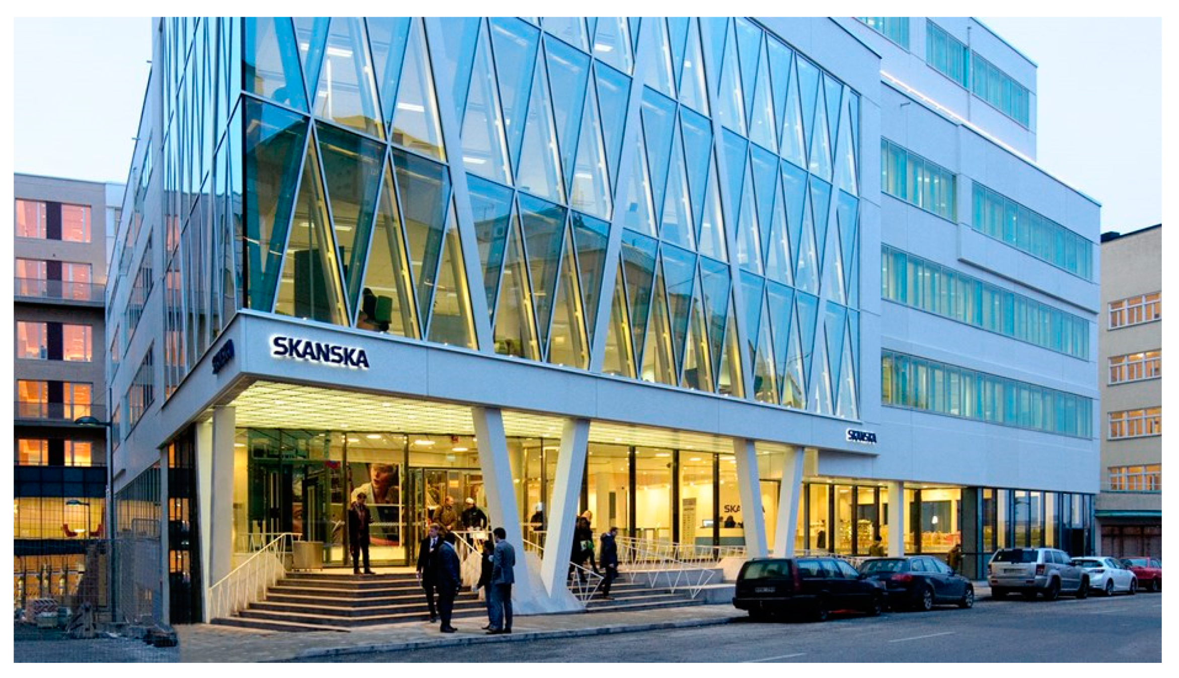
The data examined in this paper pertain to a portion of a large office building in Stockholm, Sweden shown in Figure 1. The building block consists of office spaces with only a marginal share of technical rooms; the data has been gathered only from the office spaces. These lie on 8 floors, with a total heated area of 19,642 m2. The building was constructed in 2014 and has been awarded Triple LEED Platinum certificate; according to the building owner, the number of occupants is in the order of 1000 persons.
The energy consumption data were collected from January 2014 to March 2019, with 5 min time step; they comprised external temperature measured in different locations, cold and hot water consumption, district heating, facility and tenant electricity load, free cooling pumps, room temperatures, ventilation devices and controllers, air pumping for humidity control, indoor air quality control, and air heating. The temperature sensors’ precision was ±0.1 °C, while that of electric consumption loggers being 0.1 kW.
Due to the high collinearity between most of these predictors (which is addressed in preprocessing, Section 3.1), in this paper we shall address only the tenants’ consumption measurements, which were obtained via a common meter for the appliances’ plug load and space lighting. The appliances included were those typical of an office work environment, namely personal computers, printers as well as fridges, microwaves, and coffee machines in the kitchens.
2.1. Data Preprocessing
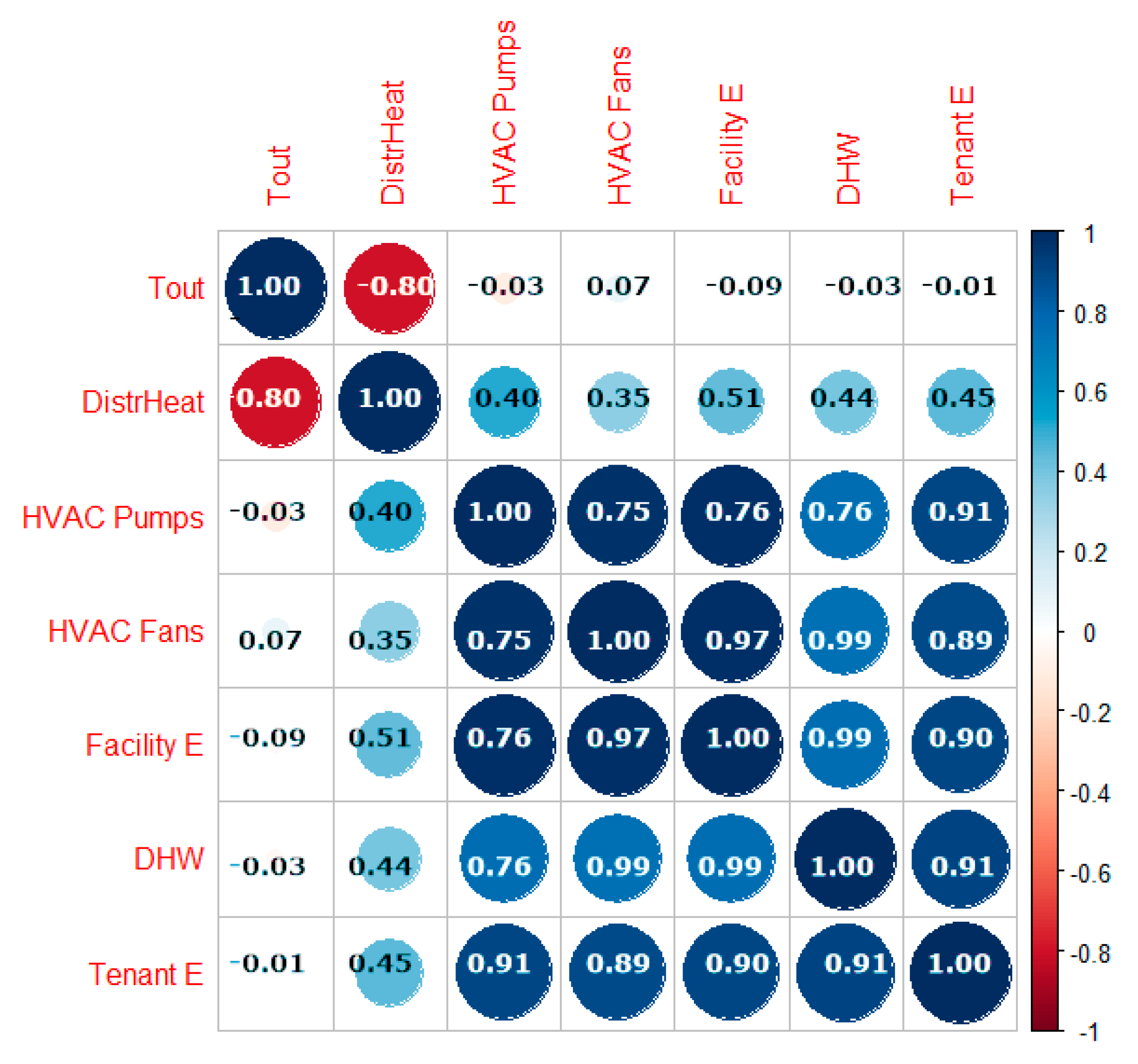
The data analysis was performed with the software R [28], through various packages. Considering the full set of variables, we checked for the existence of near-zero variance and computed correlations between the 7 predictors, obtaining the correlation matrix in Figure 2.
Preprocessing relied on probability distributions of measurements, which were built and analysed with several methods, for instance normality tests such as the p-p and Shapiro–Wilk tests. We smoothened the data with a simple moving average that was computed by averaging five values at a time. The time variable was also rescaled and normalized between 0 (=0:00) and 1 (=24:00), with 12 o’clock equal to 0.5, to reduce the sensitivity to the rounding of digits.
For the daily energy consumption, we could estimate and fit with good precision the most suitable data distribution with the aid of the Cullen and Frey graph, as well as the QQ and PP plots.
2.2. Statistical Analysis of Energy Consumption
For modelling energy consumption towards a predictive model, we compared different approaches, namely common least squares regression and a Bayesian approach [10,16,24,29]. The latter used a Monte Carlo-Markov Chain (MCMC) method to obtain posterior predictions. In other words, we generated a random binary sequence (Monte Carlo), which was then ordered by means of a constant transition matrix where the i-th event depended only on the (i-1)-th event (homogeneous Markov Chain).
First, for the regression we chose a generalized linear mixed-effects model (GLMM) model, which adds random effects (by means of a matrix Z that encodes deviations in the predictors across specified groups) to the fixed effects addressed by Generalized Linear Models (GLMs). In a frequentist analysis, the Z matrix coefficient b is regarded as a random error term.
For Bayesian inference, we assumed a normal distribution for the smooth data, consistently with our findings (see Section 3.2). Additional care needed to be adopted regarding the target average proposal acceptance probability during fitting, since the default value 0.95 lead to 34 divergent transitions. A larger value of 0.99 corresponds to a smaller step size used by the numerical integrator, thus it made the sampling more robust compared to the default value. The simulation used 30,000 iterations for increased accuracy.
The MCMC predictions were then compared with another popular regression method, the cross-validation (CV) approach [30]. Generally speaking, k-fold CV consists of randomly splitting the data into two sets: one that is used to train the model (e.g., 75% of data) and the test set, the remaining data (25%) that are used to test the model. The process is repeated k-times, and the model can be trained with a variety of methods; here we used the Metropolis algorithm that uses MCMC as well. We thus split the data into Train (75%, 56 observations) and Test (25%, 17 observations) subsets, and then used a k-fold CV with k = 10 and a cubist fit model (i.e., a rule–based model that extends Quinlan’s M5 model tree, see [31] and [32]).
2.3. Seasonal and Monthly Correlations
For addressing seasonality and weather correlations, the outdoor temperature was recorded every 5 min by a sensor installed on the outer facade of the building, while sunshine duration data were retrieved from the database [33]. In the following, every “monthly” datapoint (temperature, consumption, etc.) refers to hourly-averaged measurements covering the entire 5 year period, from 2014 to 2018.
Correlation coefficients and matrices for energy consumption versus climate were computed, together with the Pearson coefficient and an additional Kendall test. Since the latter is more sensitive than the Pearson test, we deemed it more suitable for drawing the monthly correlation matrix. The main R functions and packages that were used in this work are listed in Table 2.
3. Results
In this section we shall report the data analysis in detail, using a descriptive step-by-step approach guiding the reader through the development of a simple method for generating energy consumption profiles for application in BPS.
3.1. Data Preprocessing
First of all, we checked that the full set of seven predictors showed no problematic elements with near-zero variance. Using hourly averages of data consumption over the entire measurement period 2014–2018, we obtained the correlation matrix in Figure 2.
The mean outdoor temperature has units of [°C], all the others have [kW] units. +1 means high (perfect) correlation, −1 perfect negative correlation, with 0 meaning no correlation. Specifically, one can notice that HVAC system and facility electricity are highly correlated (at order ~ 0.98), as expected; correlations with tenants’ consumption (0.90) and DHW (0.76) are high as well. Tenants’ consumption and DHW are highly correlated too, with value 0.91.
Such high collinearity simplifies the analysis remarkably, since one can reduce the set of predictors and safely investigate only the tenants’ energy consumption.
Noticeably, on the other hand, strong negative or null correlations do exist. Clearly the outdoor temperature has −0.8 (thus, highly negative) correlation with district heating, however with HVAC, DHW, and tenants’ consumption this is very weak, ~0.02. We will address the influence of outdoor temperature and sunshine hours on tenants’ plug loads in detail in Section 3.3.1.
3.2. Daily Energy Consumption
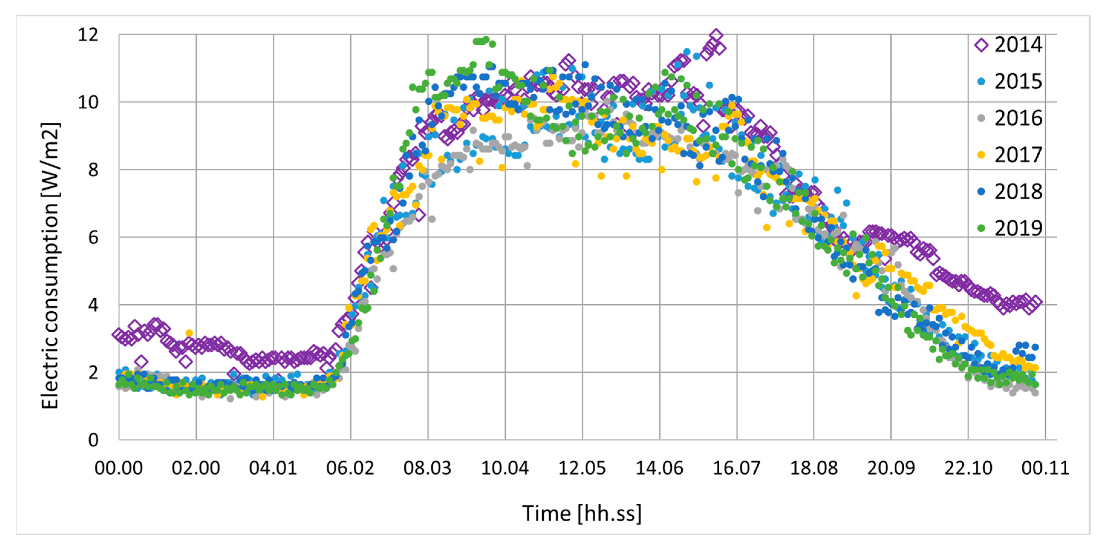
Let us begin by analysing the measured tenants’ energy consumption per square meter for a single day, which will provide a benchmark with good time resolution as the data were collected every five minutes. Measurements for Wednesday (middle-week working day) of a central February week (large occupancy) from 2014 to 2019 are plotted in Figure 3. Specifically, in this section we shall analyse Wednesday Feb 18th, 2015 as it does not deviate too much from the general trend, yet it constitutes a nontrivial example due to some outliers (at about 14:52).
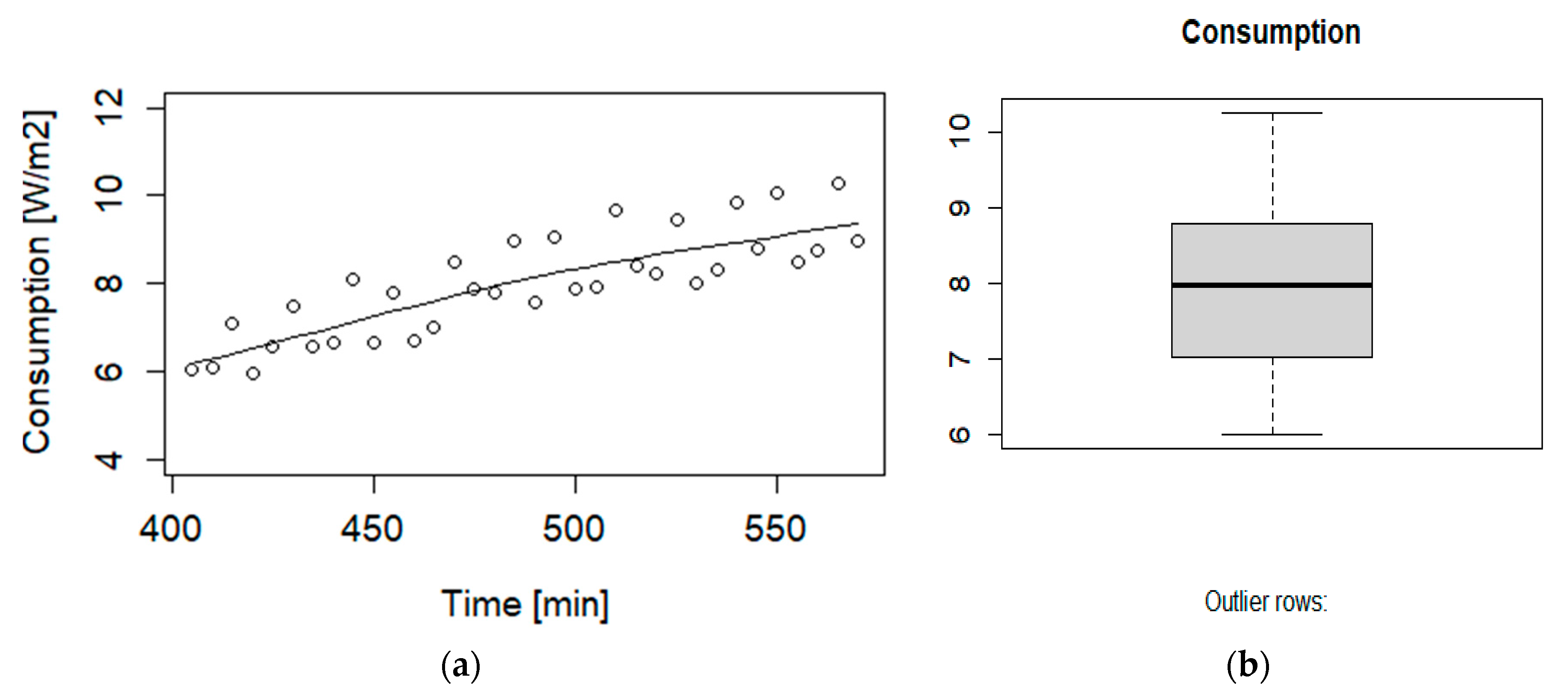
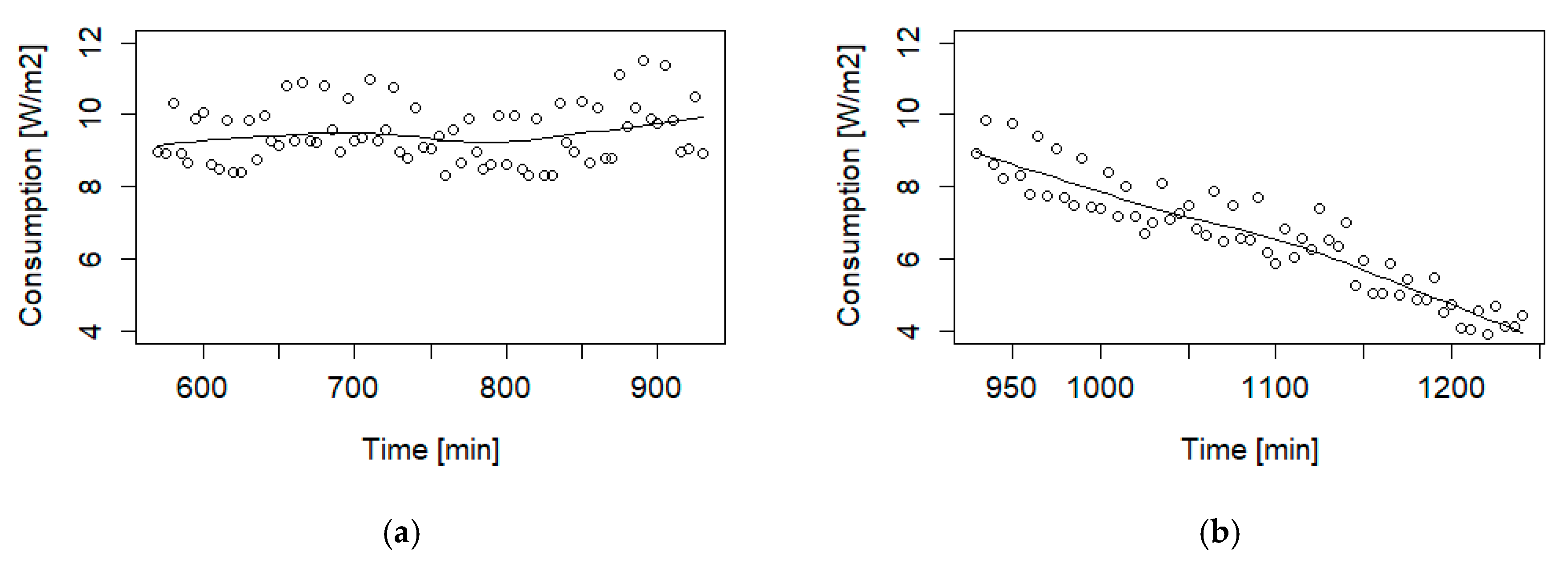
The raw data showed a large dispersion during daytime. The maximum value was found at ~3 pm, holding as 11.49 W/m2. Since we were interested in the occupied hours, the time interval was narrowed between ~7 AM and 10 PM. Following the classification scheme of the time periods in a typical working day by Zhou et al. [24], we divided the working day into three subperiods, namely 1. Arriving-at-work, 2. Daytime, 3. Off-work. The scatter and box plots for Arriving-at-work (6:45–9:30) hold as in Figure 4, featuring also, as a reference, a smooth curve fitted by Loess (a local polynomial regression that is controlled at each point by the nearest data [42]).
We recall that an outlier is any datapoint that lies outside 1.5 times the inter quartile range (IQR), which is the distance between the 25th percentile and 75th percentile values for that variable. In other words, there are no outliers here. Moreover, the correlation coefficient between time and consumption was 0.83, which is satisfactory, indicating that the trend is approximately linear.
For Daytime (09:30–15:30) we obtained instead a very scattered plot, with a low correlation holding as 0.13. The measurement error was computed as 0.61 W/m2; therefore, it is clear from Figure 5 that many outliers were present.
For the Off-work period (15:30–22:00), the box plot did not show any outliers; however, the correlation was 0.13. To understand the data distribution and compare our measurements with those of similar cases such as [24], we thus performed further tests on the daily dataset.
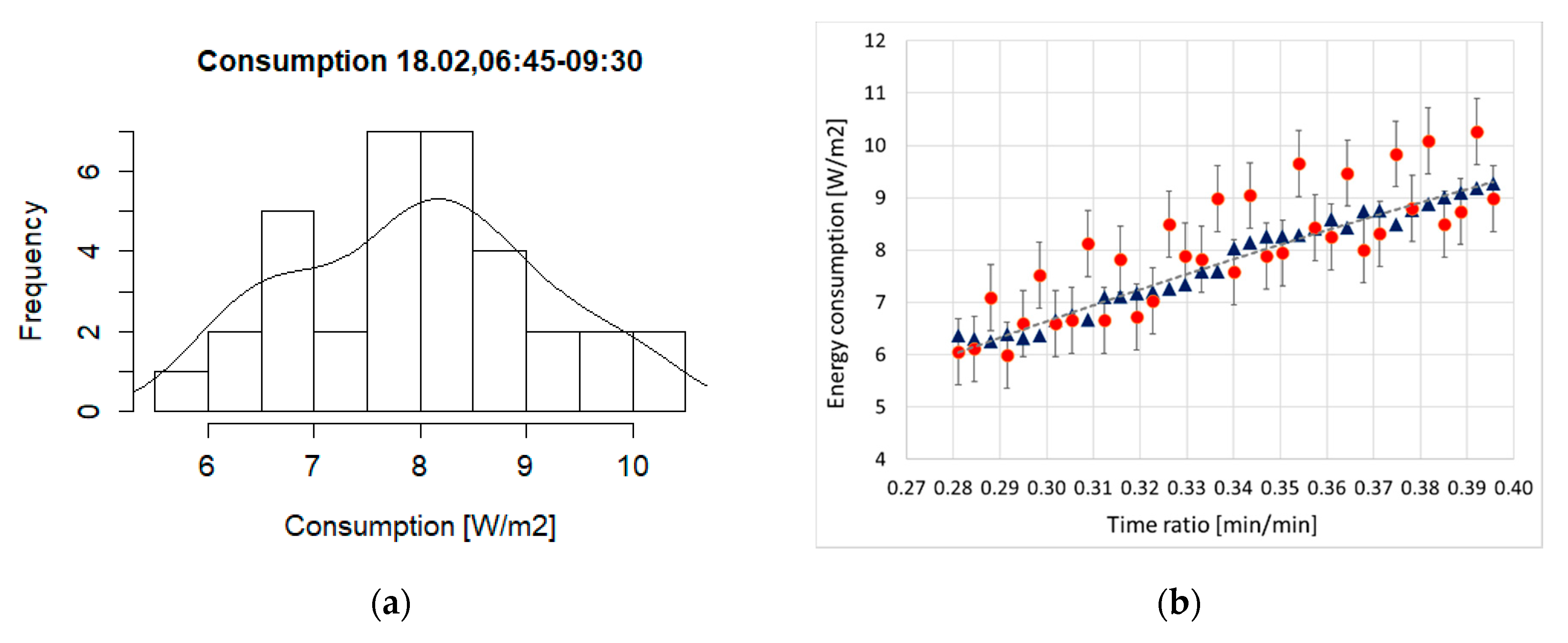
The Arriving-at-work data (06:45–09:30) in Figure 6 correspond to a distribution with median 7.97 and mean 7.996. The estimated standard deviation (sd) is 1.176, with skewness and kurtosis holding as 0.052 and 2.27, respectively. The low skewness confirms a standard (symmetric) normal distribution, while the kurtosis approaching the value of 3 means that there are no outliers, or that the tails are well-behaved. This confirms the box plot in Figure 4.
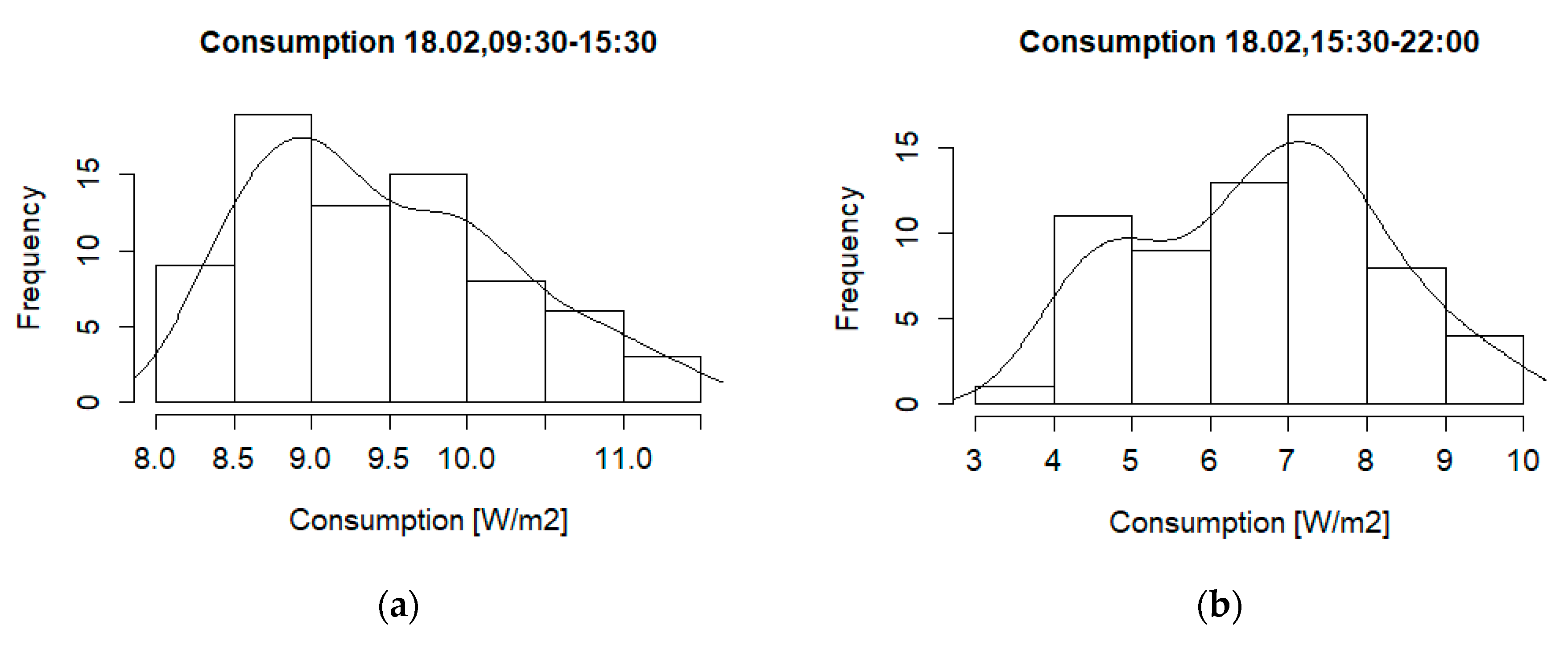
For the Daytime data (09:30–15:30), we find a median of 9.29 and a mean of 9.47. The estimated sd is 0.816, with skewness 0.569 and kurtosis 2.51. The kurtosis is still close to 3, thus we confirm the absence of outliers for this case too. The positive skewness is however ten times larger than for the symmetric normal distribution, namely this dataset corresponds to a right-skewed distribution.
Finally, the Off-work period gives a median of 6.72, a mean of 6.65, sd = 1.538, and a negative skewness −0.008, with kurtosis 2.25. The distribution is indeed very slightly left-skewed, again with no outliers.
The three normal distributions in Figure 6 and Figure 7 are therefore symmetric and right- and left-skewed, respectively, see e.g., [43]. These differ from Zhou et al. [24], who instead found Poisson for the Arriving-at-work and Off-work periods, and Normal for Daytime. This might be due to the tenants’ appliances and lighting energy usage being aggregated together since no other qualitative differences seem to distinguish the two cases.
3.2.1. Least Squares Interpolations
Aiming to generate fitting curves for predicting the measured daily energy data, we preprocessed the measurements as illustrated in Section 2.1. A comparison of smooth and original datasets is given in Figure 6.
The Daytime dataset (9:30–15:30) was then cut into subperiods because it is the most difficult period to interpolate. Fitting the smooth data with least squares returned the formula for the five subperiods as E [W/m2] = a + bt + ct2 + dt3 + et4, t ϵ [0,1], with coefficients listed in Table 3.
3.2.2. Statistical Inference of Energy Consumption
As illustrated by the R2 values in Table 3, a common least square regression could fit the smooth data for a winter day with good accuracy. Comparison between predicted and measured cumulative value [MWh] results in only a 4.7~5% difference indeed. This was possible because of the well-known property that any curve can be approximated by n parabolas, if n is sufficiently large.
As much as this is common practice, we wondered whether it was instead possible to obtain a fit for the daily dataset as a whole curve. We therefore adopted a Bayesian approach and attempted to model the dataset with this alternative prescription.
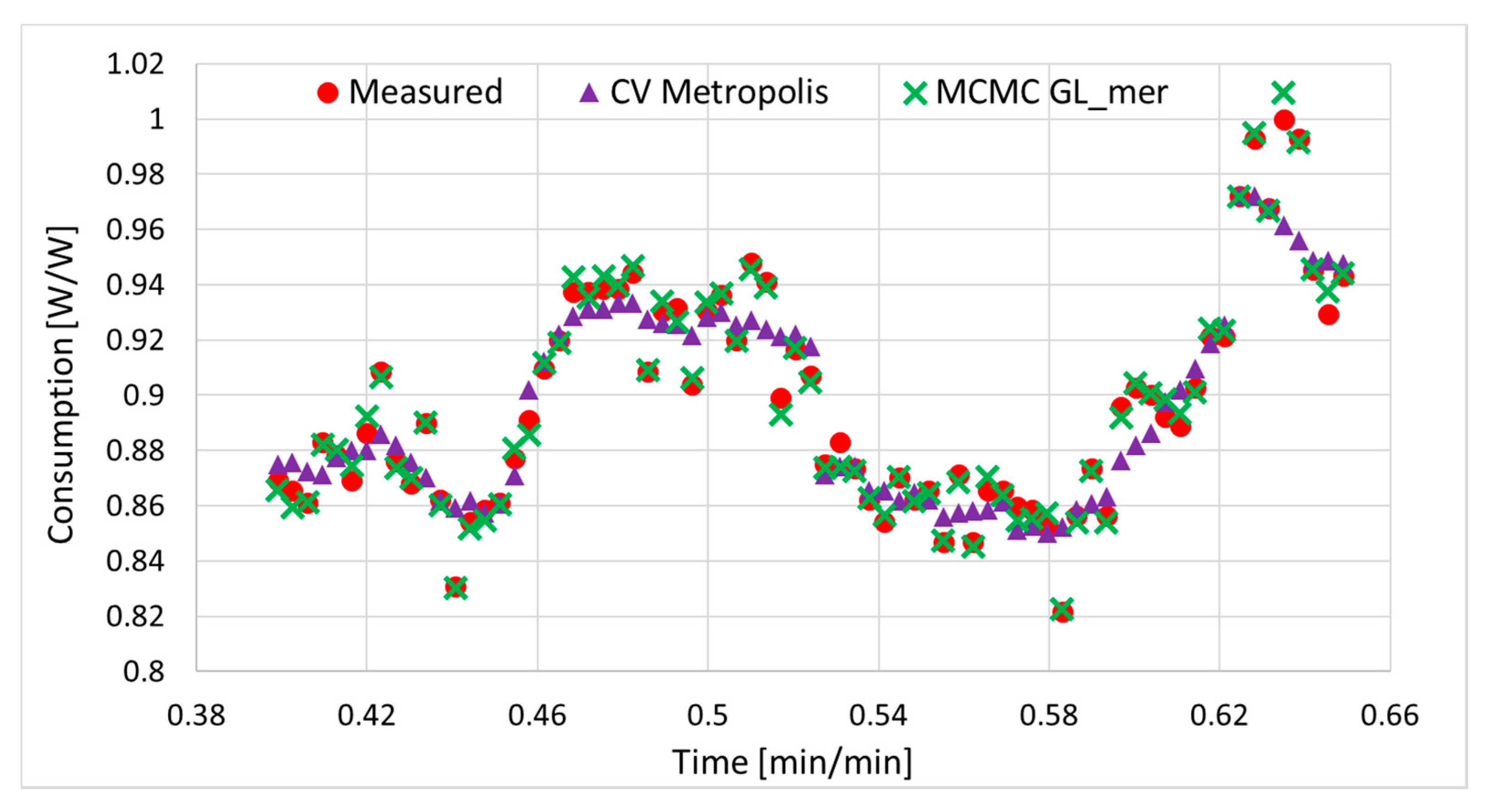
Comparison of measured data with predictions from both MCMC and Cross-Validation methods is given in Figure 8. A 10-fold cross validation managed to reproduce the observations rather well, while the overall profile looks more regular; remarkably, MCMC with GLMM could instead match even the outliers with no overfitting. MCMC had an MSE = 1.13 × 10⁻⁵, corresponding to a RMSE of 0.0033; cross validation instead reported an MSE of 1.66 × 10⁻⁴ and an RMSE of 0.0129. We obtained R2 = 0.903 for the train set and R2 = 0.926 for the test set, with a very small overfitting −0.0227. CV underestimates the energy consumption by only 0.12%, while MCMC overestimates it by 0.01%.
3.2.3. The Structural Dataset for Daily Values
The distributions for January weekday and weekends look very similar, while for June the weekend shows a sharp difference in the peaks’ ratio. From the comparison in Figure 9, clearly one cannot use the daily profile that was analysed and fitted in the previous sections, as the trend deviates qualitatively from that of other typical days.
On average, the peak consumption occurred mostly at around 9:30 (Figure 9), rather than at 15:00 (as on Wed 18.02). As a representative day we accordingly chose Wednesday 24 January 2018 (middle of the week, out of holidays), aiming to reflect an average daily profile for weekdays without the outliers appearing for the February day in Section 3.2.1.
Interpolating the January measured values with a standard least squares method returns a 2.1% difference in total energy consumption between fit and measurements, which is satisfactory. However, for higher accuracy and for reasons that will be explained in Section 3.3.2, the coefficients listed in according to the generic formula E [W/m2] = a + bt + ct2 + dt3 + et4, t ϵ [0,24) were obtained with a nonlinear analysis, by applying to the fit an “energy constraint” that minimizes the difference between observed and fitted values [26] (the round bracket at t = 24h ensures that midnight is not overcounted). Moreover, we demanded that the fitted values at the joining points (at 9 AM and 3 PM for weekdays in Table 4) differ by less than 0.01 W/m2. The according constrained fit returns an observed/fitted difference of only 0.05% for the January consumption; it will be called “structural curve” henceforth.
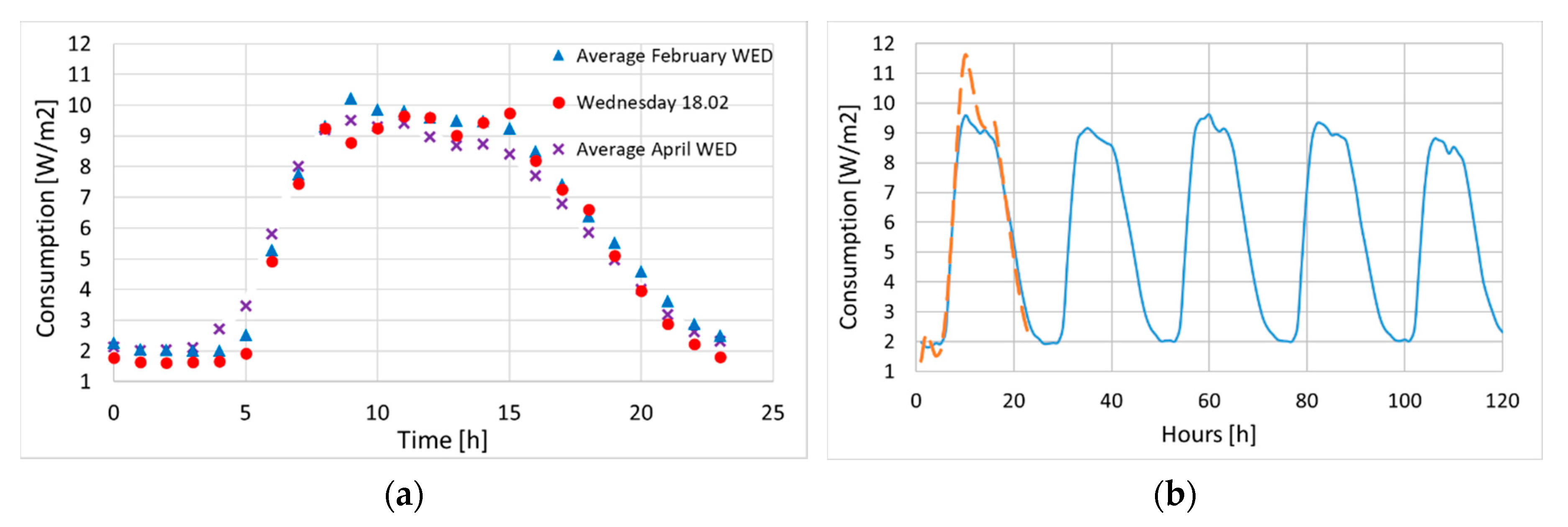
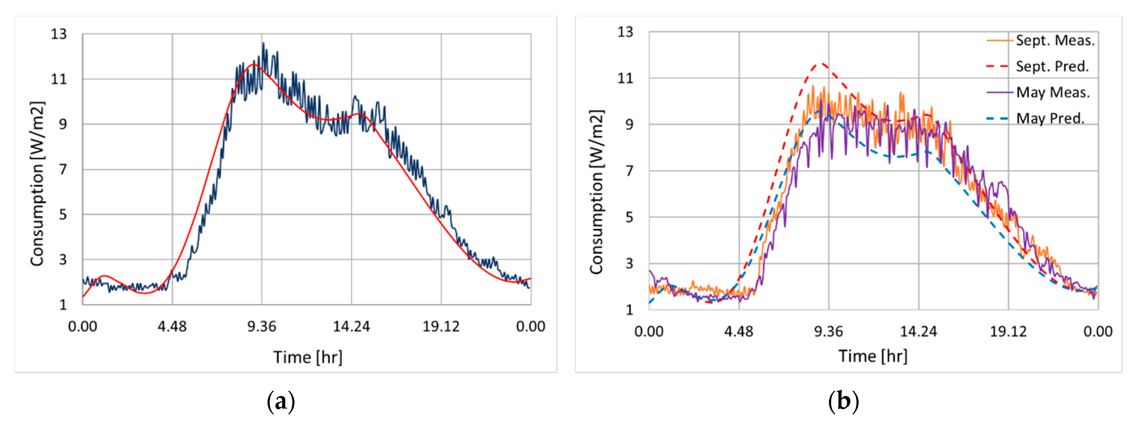
In Figure 9b, the structural curve is compared to the energy profiles computed by averaging the data, hour by hour for each day, over all the working weeks from 2013 to 2018. While the prediction does overestimate the peak value, the overall trend is clearly matched by the structural curve; such overestimation is expected, since averaging over large ensembles always reduces peak values. Predictions for two random May and September weekdays are compared with data in Figure 10.
For the weekend instead we fitted energy data from an average profile, since the Saturday and Sunday curves had a large variety of trends thus a specific representative could not be identified. The Weekend fit reported in Table 4 matches the daily consumption within a ~5% error.
3.3. Monthly Energy Consumption
In this section we first briefly analyse the energy consumption data on a monthly basis, then based on the January profile in Table 4 we evaluate correlation formulas for all the 11 remaining months, which are to be used as boundary conditions of BPS. The differences between months are highlighted and searching for possible weather correlations shall help in determining the impact of occupancy on energy consumption. To our knowledge, such an analysis is still very scarce in energy consumption studies of large office buildings, with the only exception of [44].
Averaging the hourly power [kW] over each month and then dividing by the corresponding February consumption gives the ratios in Table 5: February is the month showing the largest consumption. Since a striking as well as expected difference exists between autumn/winter and summer months, one might wonder whether this is correlated to weather or to occupancy.
3.3.1. Seasonal Variations
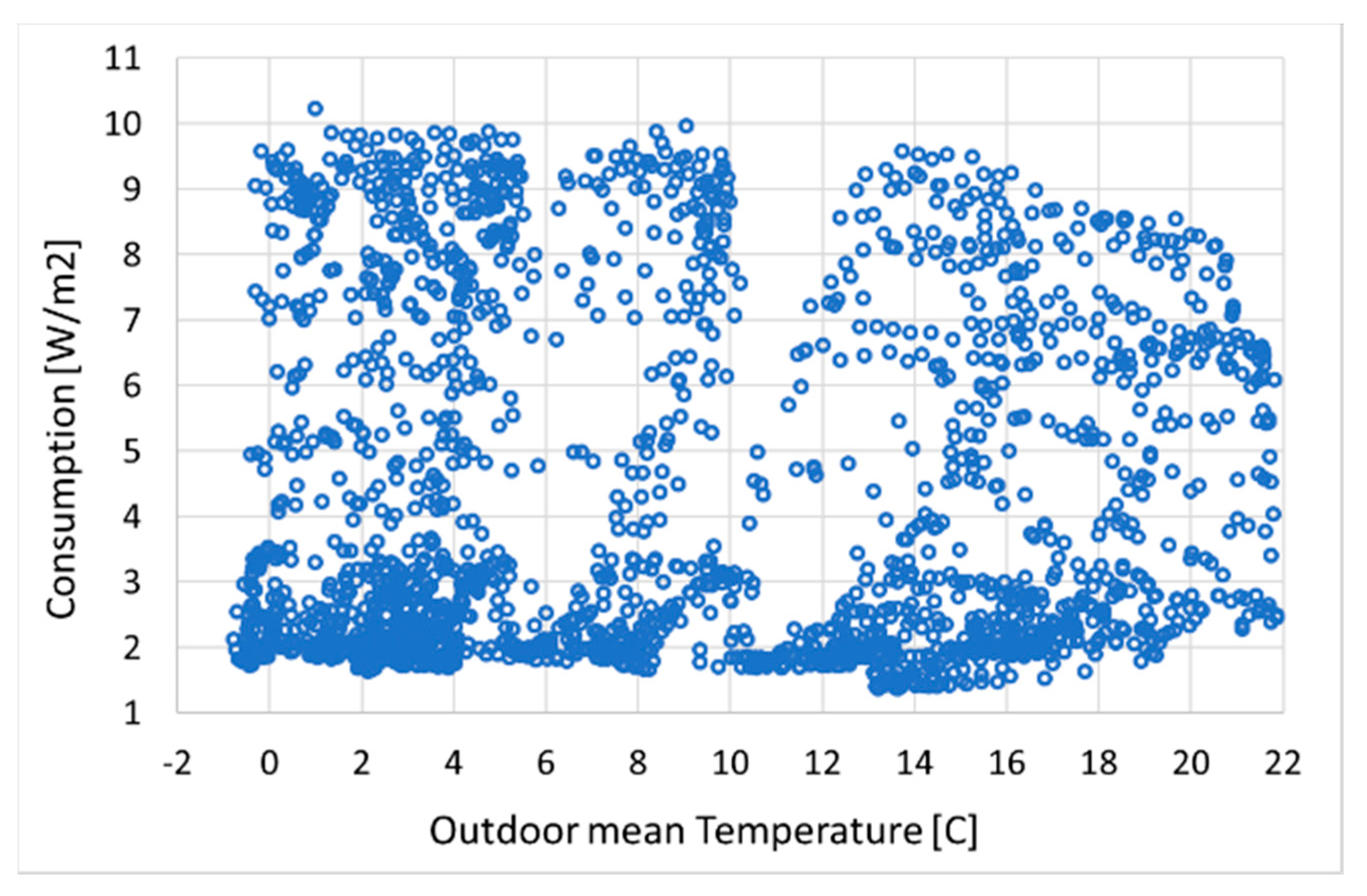
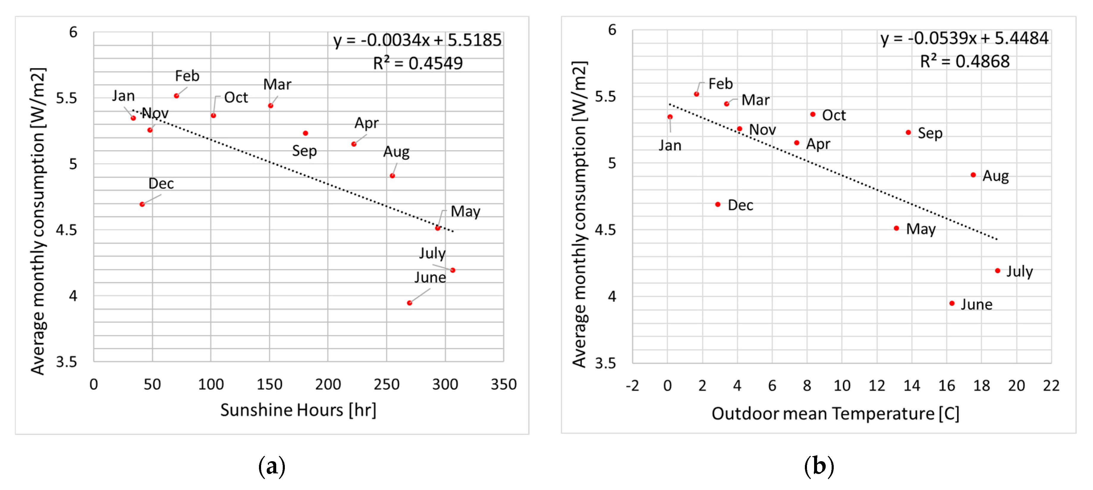
It is easy to see that weather and consumption are weakly correlated, as it is shown in Figure 11, Figure 12 and Figure 13 for consumption vs. measured irradiation hours and average outdoor temperature. The measurements are averaged over the entire period 2014–2018. This is confirmed by an additional Pearson test, which holds respectively as –0.67 and –0.70, as well as by the values in Table 5.
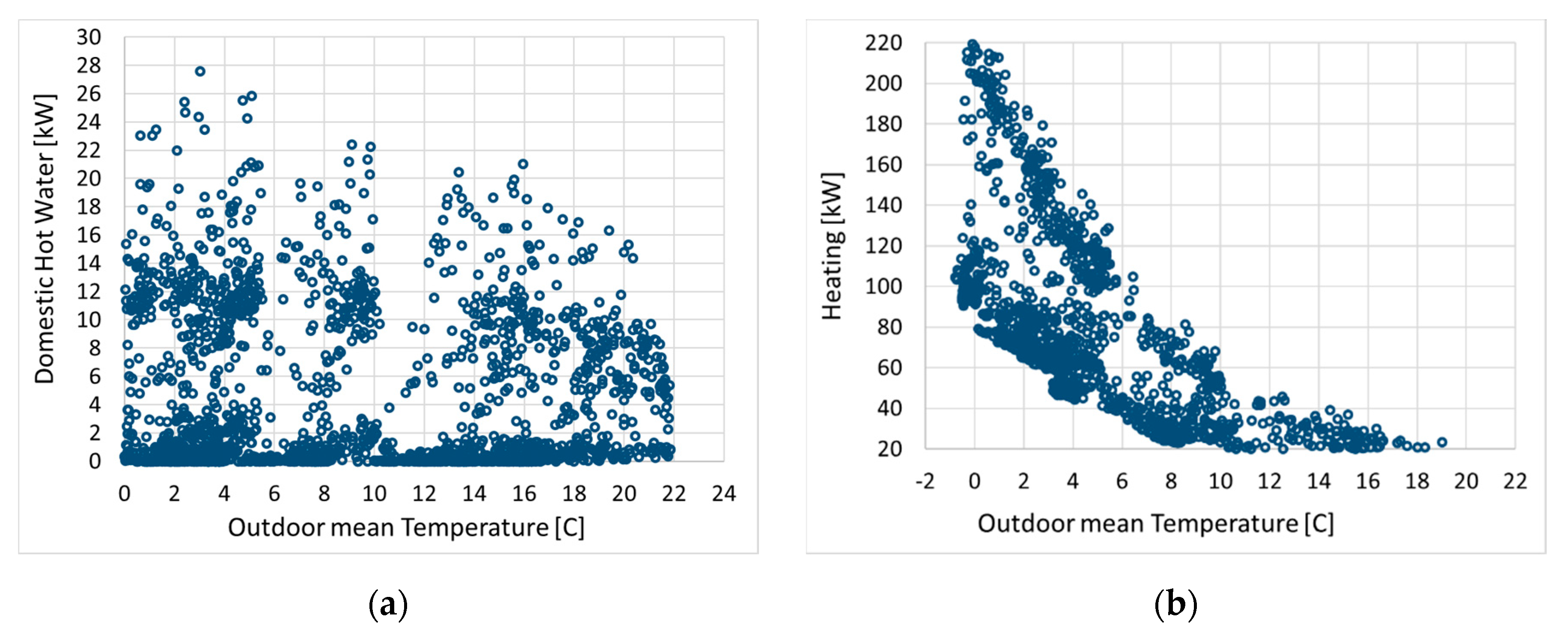
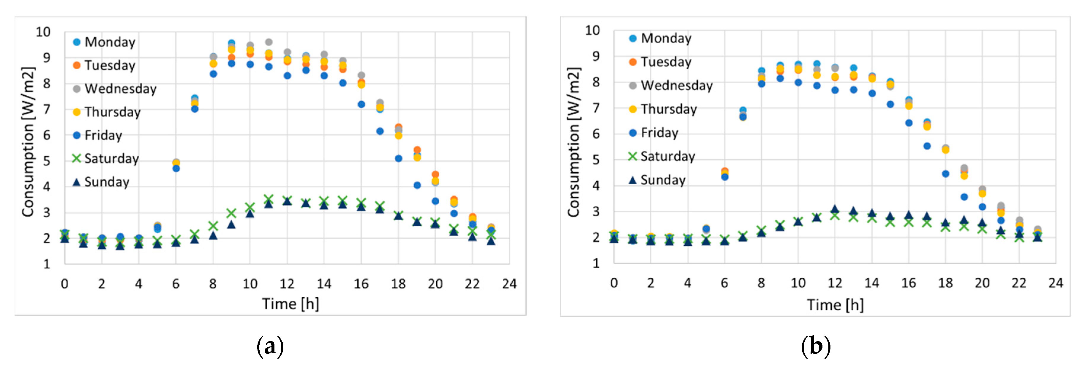
Domestic hot water (DHW) consumption is also independent of the external temperature, while only air heating shows a clear correlation as expected, as illustrated in Figure 12. More into detail, Figure 14 considers two specific days in winter and in summer. As a reference for an average winter profile, we chose one week in January (the coldest month). Hourly averages for the consumption data are averaged for the same weekday at each week of the month.
3.3.2. Monthly Correlations
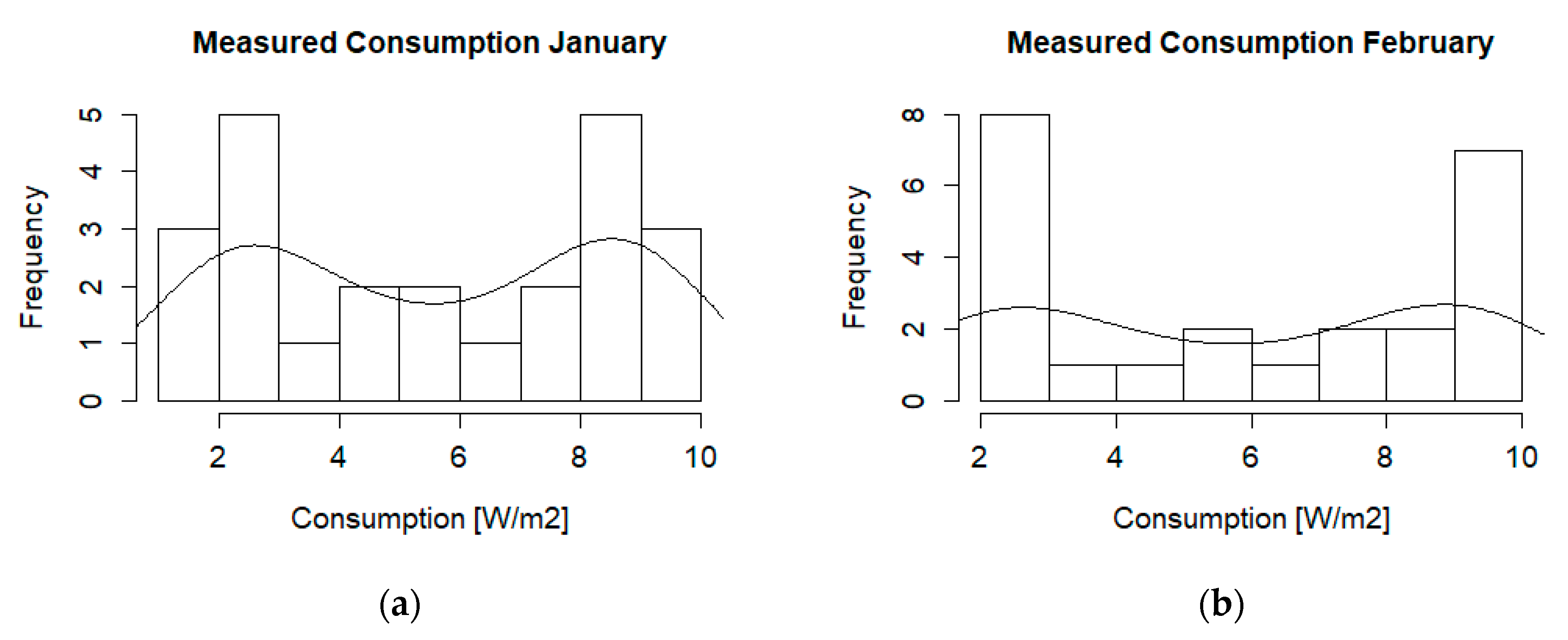
The density distributions of consumption data (hourly values averaged over 2014–2018) are very similar to each other, the only exception being February, see Figure 15.
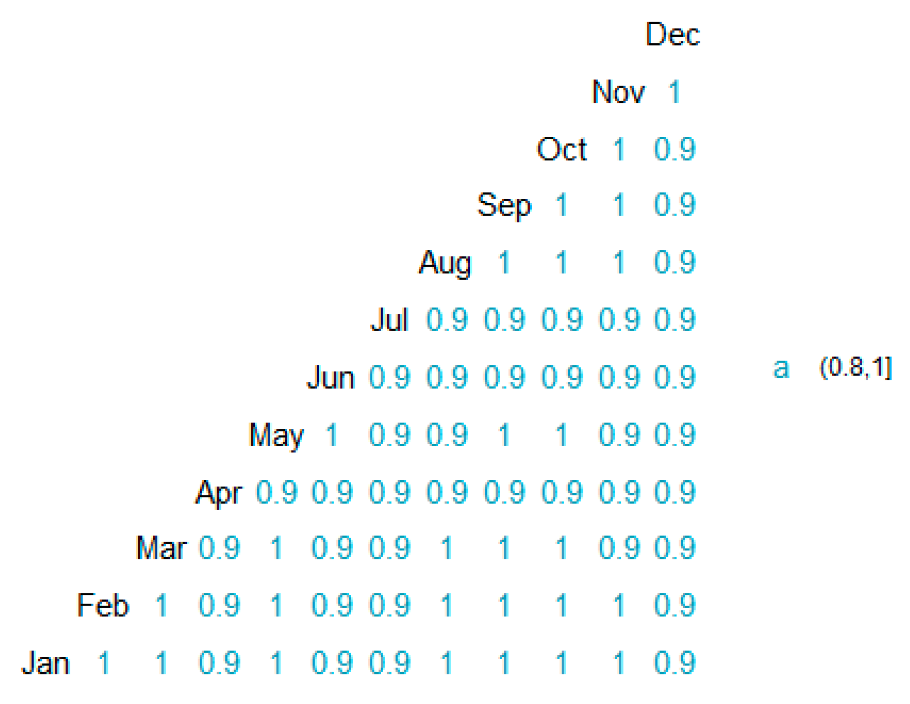
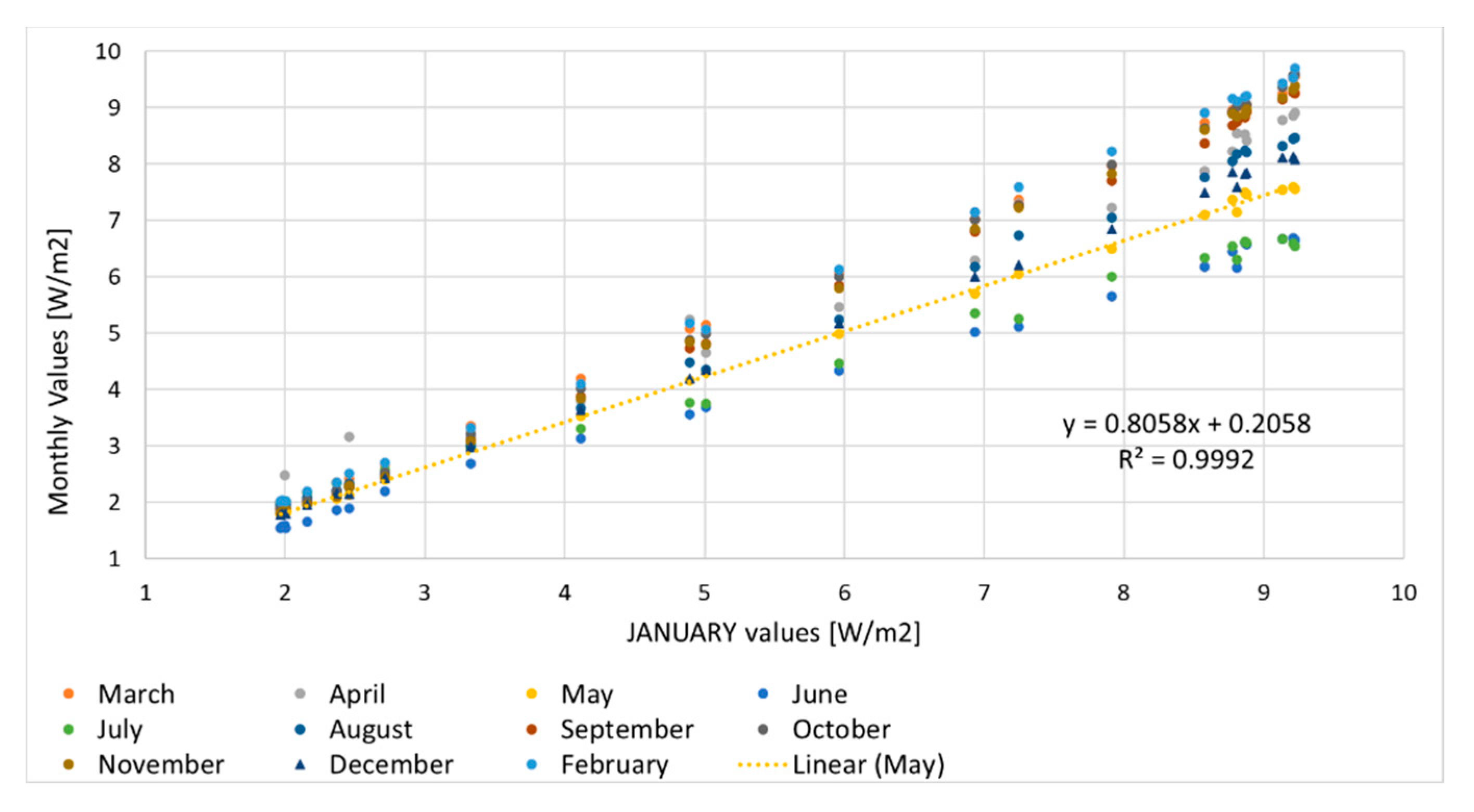
Interestingly, one finds a strong linear correlation between months, as shown below by the correlation matrix in Figure 16. The “1” entries are due to rounding of R-squared values that are very close, yet obviously not identical to unity. Correlation coefficients for each month against January, which constitutes our structural dataset, are provided in Table 5 for both weekdays and weekend.
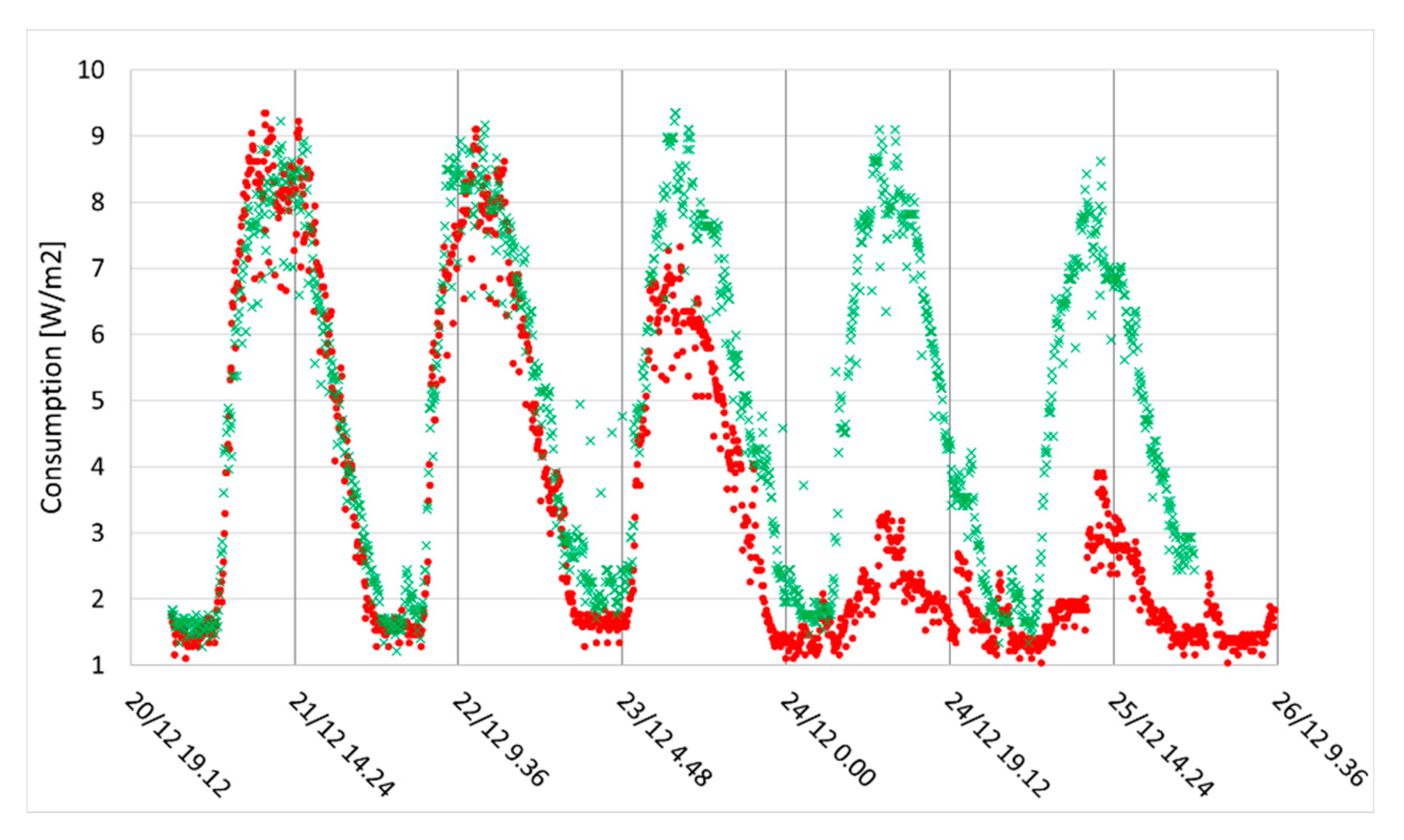
The numerical values are computed with the Kendall test, that is more sensitive than the Pearson test. The correlation is very strong, only April has a couple of outliers in Figure 17, where each month is plotted against January (the interpolation formula holds for May, as an example). We also wondered about the role of the Christmas holidays, which are distributed less evenly than summer vacations: Figure 18 addresses the working week starting on Dec 21st and ending at Christmas, which is compared to a Summer week (last working week of June).
At this point, let us recall that we aim to obtain formulas for a prompt implementation in BPS software. One immediate option would be to simply produce interpolation formulas for each month as in Table 4 and list them in 12 tables, with a loss in generality; here we prefer a more general and time-saving approach that is described in the next section.
3.3.3. The Monthly Structural Dataset and Prediction Formulas
Following Ref. [26] and using its terminology, we first identify January as our representative month with its structural dataset, then derive for each other month the according correlation formulas with January, written in the form E[W/m2] = A × EJan + B, from the according measured consumptions as in Figure 17. Now one needs only to input the interpolation coefficients for January (Table 4) and the correlations for each month (Table 5) into any simulation software, then proceed with, e.g., annual simulations of energy consumption.
This is a very simple method, based on linear interpolations, which naturally returns only a small sensitivity on the coefficients, as well as a small error (see [26] for a more detailed discussion). January is chosen because, according to Figure 16, it is the month with the highest correlation with any other month.
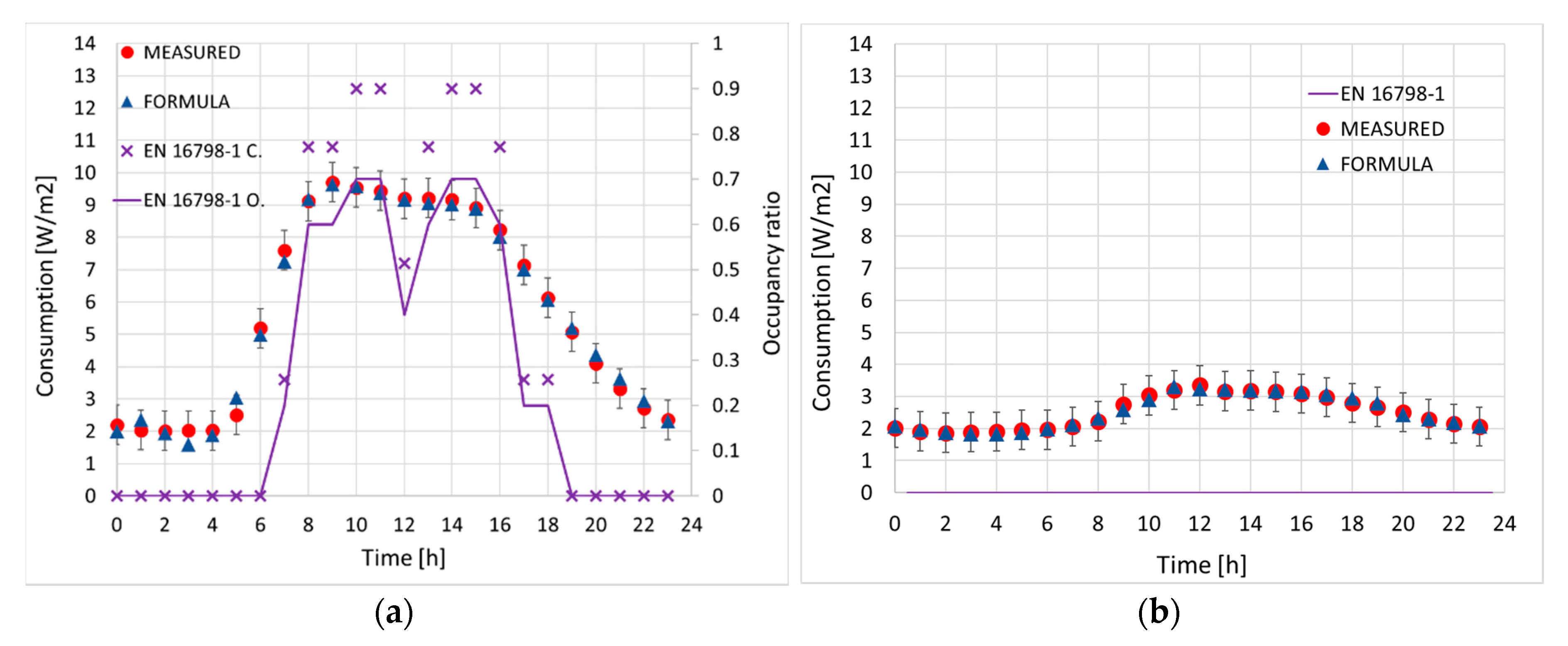
Let us immediately test this approach by comparing June measurements (24 hourly averages over weekdays), with error 0.61 W/m2, with the values obtained by means of the correlation coefficients in Table 5. For generating the average January weekday profiles, namely the 24 hourly EJan values, we shall use either linear regression (Table 4) or MCMC (Figure 8).
Figure 19 shows the result for June, when using the January structural coefficients in Table 4. The agreement is excellent, with every point within the experimental error and an average % residual of 3.7% for weekdays, 2.46% for weekends. Using instead Bayesian inference (MCMC here) to compute the structural dataset lowers the average % residuals to resp. 1.83% and 1.7%.
The plot in Figure 19 also features purple crosses, i.e., the hourly consumption computed according to the occupancy profile (solid purple line) of the EU Standard EN 16798-1 [25]. The Standard estimates 12 W/m2 for lighting and 6 W/m2 for occupancy, neglecting the weekends completely and assuming null occupancy throughout. We thus conclude that in this case one cannot infer energy consumption directly from the EN 16798-1 occupancy profile.
This is confirmed by comparing the cumulative measured data for an average year with the profiles obtained with the structural dataset (Table 4 and Table 5), that gives a 4.69% overestimation of the total consumption when using our formulas. On the other hand, simply assuming the occupancy profile from the standard EN 16798-1 returns an underestimation of the real consumption of the order ~27%.
Comparison with the yearly accumulated consumption for each year is given in Table 6 (the year 2019 was not considered as the data were recorded only until 20th March).
4. Discussion
The daily energy consumption analysed in Section 3.2 showed some peculiar characteristics. Interestingly, the distributions for each period were different for the analogous cases of large office buildings in China [24] and in Austria [10]. While one cannot be sure whether this is due to geographical differences (lighting component) rather than to appliances usage, this combined evidence might suggest that generalizing consumption patterns of a building typology at an international level is not as immediate as it seems.
Besides, we have shown in Section 3.2.1 that fitting the data for a nontrivial profile with the good old minimum square method returned an error of only ~5%, in agreement with [18]. A more sophisticated Bayesian approach showed an even higher accuracy, with error well below 1%. In other words, it is quite feasible to model this type of energy data with high accuracy even with simple methods; models should be conveniently chosen according to the specific BPS.
Regarding the seasonal variations and weather correlations, the preprocessing showed that there exists a high collinearity between the electric consumption of facility and HVAC system. Furthermore, these are highly correlated also with the DHW and tenants’ appliances power plug and lighting consumption. Only the district heating is (negatively) correlated with the outdoor temperature, as expected. These results are accordingly pointing at occupancy as the main cause of energy consumption fluctuations in the building.
More specifically, one can notice the low R-squared values for a linear fit in Figure 13, showing low correlation with the climate. Consumption is indeed larger in August than in December and May, and in March compared to January. December, June, and July, i.e., the holiday months, are particularly intriguing: June and July incidentally have smaller consumption as well as higher temperatures/irradiation. Interestingly, May recorded about the same irradiation yet larger consumption. Accordingly, comparing these two plots might also suggest a more prominent role of plug load (i.e., of occupancy) than of lighting.
January weekdays are almost indistinguishable from each other, with the only exception being Friday (Figure 14). The weekend is slightly more interesting, as Saturday’s curve is different from Sunday’s. It can be shown that Monday and Tuesday have a similar density distribution, as well as Wed, Thu, and Fri; the daily consumption has anyway little variations within each of the two sets (weekdays and weekends). These considerations are consistently valid for all the twelve months, with little variance. Interestingly, the according distributions are all skew normal, in contrast with the profiles plotted in Wang [16] and Ding [29] for large Chinese buildings. We can speculate that this might be due to the plug loads and lighting being aggregated together.
Identifying the structural dataset and computing the structural curve followed the principles explained in [26]. The specific dataset reflected the general trend qualitatively: looking for common patterns in the full data is the most important step in the analysis. Choosing, e.g., the February day analysed in Section 3.2.1 and Section 3.2.2, with its outliers and peaks at ~3 PM, would have determined a different outcome at least in terms of daily consumption distribution, if not of annual energy simulation. Since instead the Weekend profiles were highly different for all the five years considered, we used a profile that was constructed by averaging the hourly values over the full dataset. We shall finally remark that here we showed only one way to obtain the structural curve, for illustrative purposes: any other method can be equally valid, since a whole class of very sophisticated statistical models already exists, as summarized in Table 1.
5. Conclusions
As building performance simulations constitute an increasingly common practice among engineers for assessing the energy analysis at different levels, it is needed to bridge the gap between observations and predictions with simple, yet reliable approaches for the implementation into BPS that are suitable to academics as well as to practitioners. In this paper we have argued whether this is possible, by examining the presently largest ensemble of energy consumption data of an office building in a Nordic country.
Considering the employees’ appliances plug consumption and lighting for a calendar year, we found no evident weather correlation. Rather, holiday periods and their impact on occupancy proved to be more important: the highest consumption occurred in February and the lowest in June. All the months were highly correlated.
Daily consumption patterns showed on the average a clear peak at around 9:30 AM for weekdays, while weekends exhibited a larger variance. Comparing regression curves obtained with a frequentist inference to Bayesian inference (MCMC), we obtained an extremely high accuracy with the latter; nevertheless, the least squares method returned only a 2% error, which is low enough for implementation into BPS.
These results lead to the definition of an analytical bottom-up model, for predicting any daily consumption given a benchmark daily profile with an error smaller or equal to 5%. On one hand, the numerical coefficients reported in Table 4 and Table 5 can be immediately implemented into building performance simulations addressing comparable datasets.
More in general, we believe that the procedure detailed in Section 3.2.3 and Section 3.3.3 is a simple yet effective analysis blueprint that can be directly employed in energy consumption assessments and BPS modelling of a variety of building, location, and study typologies. The flexibility of the original method, which was postulated for DHW consumption data of residential buildings [26], should be evident from the present context, where it was adapted to a case study with very different datasets.
In conclusion, this paper analysed a substantially large amount of data obtained during five years of measurements, addressing tenants’ plug load and lighting consumption when aggregated together. Further studies should investigate the role of tenants’ plug load when it is aggregated separately, how different occupancy models could impact the overall energy use, and how the prediction model benefits investigations through BPS by applying the structural dataset method to, e.g., annual simulations with IDA ICE and other simulation programs.
Author Contributions
Conceptualization, A.F., H.K., J.K., and M.T.; methodology, A.F. and M.T.; software, validation, formal analysis, investigation, A.F.; data curation, A.F. and H.K.; writing—original draft preparation, A.F.; writing—review and editing, A.F., J.K. and M.T.; supervision, J.K. and M.T.; project administration, M.T.; funding acquisition, J.K. and M.T. All authors have read and agreed to the published version of the manuscript.
Funding
The authors acknowledge support by the European Regional Development Fund via the Estonian Centre of Excellence in Zero Energy and Resource Efficient Smart Buildings and Districts ZEBE, grant 2014-2020.4.01.15-0016, and funding by the Estonian Research Council through grant IUT1-15 and the programme Mobilitas Pluss (Grant No.—2014-2020.4.01.16-0024, MOBTP88).
Acknowledgments
We are grateful to Pär Carling at EQUA Solutions AB and Jonas Graslund at Skanska AB for data acquisition and clarifications, as well as to Tuule Mall Kull for contributing to the data analysis.
Conflicts of Interest
The authors declare no conflict of interest. The funders had no role in the design of the study; in the collection, analyses, or interpretation of data; in the writing of the manuscript, or in the decision to publish the results.
References
- Hong, T.; Taylor-Lange, S.C.; D’Oca, S.; Yan, D.; Corgnati, S.P. Advances in research and applications of energy-related occupant behavior in buildings. Energy Build. 2016, 116, 694–702. [Google Scholar] [CrossRef] [Green Version]
- Delzendeh, E.; Wu, S.; Lee, A.; Zhou, Y. The impact of occupants’ behaviours on building energy analysis: A research review. Renew. Sustain. Energy Rev. 2017, 80, 1061–1071. [Google Scholar] [CrossRef]
- Zhao, J.; Lasternas, B.; Lam, K.P.; Yun, R.; Loftness, V. Occupant behavior and schedule modeling for building energy simulation through office appliance power consumption data mining. Energy Build. 2014, 82, 341–355. [Google Scholar] [CrossRef]
- D’Oca, S.; Hong, T. Occupancy schedules learning process through a data mining framework. Energy Build. 2015, 88, 395–408. [Google Scholar] [CrossRef] [Green Version]
- Klein, L.; Kwak, J.-Y.; Kavulya, G.; Jazizadeh, F.; Becerik-Gerber, B.; Varakantham, P.; Tambe, M. Coordinating occupant behavior for building energy and comfort management using multi-agent systems. Autom. Constr. 2012, 22, 525–536. [Google Scholar] [CrossRef]
- Lee, Y.S.; Malkawi, A.M. Simulating multiple occupant behaviors in buildings: An agent-based modeling approach. Energy Build. 2014, 69, 407–416. [Google Scholar] [CrossRef]
- Bonte, M.; Thellier, F.; Lartigue, B. Impact of occupant’s actions on energy building performance and thermal sensation. Energy Build. 2014, 76, 219–227. [Google Scholar] [CrossRef]
- Page, J.; Robinson, D.; Morel, N.; Scartezzini, J.-L. A generalised stochastic model for the simulation of occupant presence. Energy Build. 2008, 40, 83–98. [Google Scholar] [CrossRef]
- Richardson, I.; Thomson, M.; Infield, D. A high-resolution domestic building occupancy model for energy demand simulations. Energy Build. 2008, 40, 1560–1566. [Google Scholar] [CrossRef] [Green Version]
- Mahdavi, A.; Tahmasebi, F.; Kayalar, M. Prediction of plug loads in office buildings: Simplified and probabilistic methods. Energy Build. 2016, 129, 322–329. [Google Scholar] [CrossRef] [Green Version]
- Calì, D.; Andersen, R.K.; Müller, D.; Olesen, B.W. Analysis of occupants’ behavior related to the use of windows in German households. Build. Environ. 2016, 103, 54–69. [Google Scholar] [CrossRef] [Green Version]
- Menezes, A.; Cripps, A.; Buswell, R.; Wright, J.; Bouchlaghem, D. Estimating the energy consumption and power demand of small power equipment in office buildings. Energy Build. 2014, 75, 199–209. [Google Scholar] [CrossRef] [Green Version]
- Tetlow, R.M.; Van Dronkelaar, C.; Beaman, C.P.; Elmualim, A.; Couling, K. Identifying behavioural predictors of small power electricity consumption in office buildings. Build. Environ. 2015, 92, 75–85. [Google Scholar] [CrossRef]
- Tanimoto, J.; Hagishima, A.; Sagara, H. A methodology for peak energy requirement considering actual variation of occupants’ behavior schedules. Build. Environ. 2008, 43, 610–619. [Google Scholar] [CrossRef]
- Virote, J.; Neves-Silva, R. Stochastic models for building energy prediction based on occupant behavior assessment. Energy Build. 2012, 53, 183–193. [Google Scholar] [CrossRef]
- Wang, Z.; Ding, Y. An occupant-based energy consumption prediction model for office equipment. Energy Build. 2015, 109, 12–22. [Google Scholar] [CrossRef]
- Gilani, S.; O’Brien, W. A preliminary study of occupants’ use of manual lighting controls in private offices: A case study. Energy Build. 2018, 159, 572–586. [Google Scholar] [CrossRef]
- Gilani, S.; O’Brien, W.; Gunay, H.B. Simulating occupants’ impact on building energy performance at different spatial scales. Build. Environ. 2018, 132, 327–337. [Google Scholar] [CrossRef]
- Chen, Z.; Xu, J.; Soh, Y.C. Modeling regular occupancy in commercial buildings using stochastic models. Energy Build. 2015, 103, 216–223. [Google Scholar] [CrossRef]
- Wang, C.; Yan, D.; Jiang, Y. A novel approach for building occupancy simulation. Build. Simul. 2011, 4, 149–167. [Google Scholar] [CrossRef]
- Aerts, D.; Minnen, J.; Glorieux, I.; Wouters, I.; Descamps, F. A method for the identification and modelling of realistic domestic occupancy sequences for building energy demand simulations and peer comparison. Build. Environ. 2014, 75, 67–78. [Google Scholar] [CrossRef]
- Buso, T.; Fabi, V.; Andersen, R.K.; Corgnati, S.P. Occupant behaviour and robustness of building design. Build. Environ. 2015, 94, 694–703. [Google Scholar] [CrossRef]
- Haldi, F.; Robinson, D. Interactions with window openings by office occupants. Build. Environ. 2009, 44, 2378–2395. [Google Scholar] [CrossRef]
- Zhou, X.; Yan, D.; Hong, T.; Ren, X. Data analysis and stochastic modeling of lighting energy use in large office buildings in China. Energy Build. 2015, 86, 275–287. [Google Scholar] [CrossRef] [Green Version]
- CEN. Energy Performance of Buildings—Part 1: Indoor Environmental Input Parameters for Design and Assessment of Energy Performance of Buildings; E. 16798-1; CEN: Brussels, Belgium, 2019. [Google Scholar]
- Ferrantelli, A.; Ahmed, K.; Pylsy, P.; Kurnitski, J. Analytical modelling and prediction formulas for domestic hot water consumption in residential Finnish apartments. Energy Build. 2017, 143, 53–60. [Google Scholar] [CrossRef]
- SKANSKA AB. Entré Lindhagen. Available online: https://www.skanska.se/en-us/our-offer/our-projects/57328/Entre-Lindhagen (accessed on 29 September 2020).
- R Team. R: A Language and Environment for Statistical Computing; R Foundation for Statistical Computing: Vienna, Austria, 2013. [Google Scholar]
- Ding, Y.; Wang, Q.; Wang, Z.; Han, S.; Zhu, N. An occupancy-based model for building electricity consumption prediction: A case study of three campus buildings in Tianjin. Energy Build. 2019, 202, 109412. [Google Scholar] [CrossRef]
- Hastie, T.; Tibshirani, R.; Friedman, J.H. The Elements of Statistical Learning: Data Mining, Inference, and Prediction; Springer Science & Business Media: Berlin, Germany, 2009. [Google Scholar]
- Quinlan, J.R. Learning with Continuous Classes. In Proceedings of the 5th Australian Joint Conference on Artificial Intelligence, Hobart, Tasmania, 16–18 November 1992; World Scientific: Singapore, 1992; Volume 92, pp. 343–348. [Google Scholar]
- Witten, H.; Eibe, F. Data mining: Practical machine learning tools and techniques with Java implementations. ACM Sigmod Rec. 2002, 31, 76–77. [Google Scholar] [CrossRef]
- Josefsson, W. Long-Term Global Radiation in Stockholm, 1922–2018 (Meteorologi). 2019. Available online: http://urn.kb.se/resolve?urn=urn:nbn:se:smhi:diva-5175 (accessed on 24 February 2020).
- Kuhn, M. Building Predictive Models in R Using the caret Package. J. Stat. Softw. 2008, 28, 1–26. [Google Scholar] [CrossRef] [Green Version]
- Wei, T.; Simko, V. R package “corrplot”: Visualization of a Correlation Matrix (Version 0.84). 2017. Available online: https://github.com/taiyun/corrplot (accessed on 20 September 2020).
- Azzalini, A. Package ‘sn’: The Skew-Normal and Related Distributions Such as the Skew-t (Version 1.6-2). 2020. Available online: http://azzalini.stat.unipd.it/SN (accessed on 6 October 2020).
- Svetunkov, I. Smooth: Forecasting Using State Space Models, R Package Version 2.5. 2018. Available online: https://cran.r-project.org/web/packages/smooth/vignettes/smooth.html (accessed on 25 June 2020).
- Delignette-Muller, M.L.; Dutang, C. Fitdistrplus: An R Package for Fitting Distributions. J. Stat. Softw. 2015, 64, 1–34. [Google Scholar] [CrossRef] [Green Version]
- Bates, D.; Mächler, M.; Bolker, B.; Walker, S. Fitting Linear Mixed-Effects Models Usinglme4. J. Stat. Softw. 2015, 67, 1–48. [Google Scholar] [CrossRef]
- Goodrich, B.J.; Gabry, I.A.; Brilleman, S. Rstanarm: Bayesian Applied Regression Modeling via Stan. 2020. Available online: https://mc-stan.org/rstanarm (accessed on 12 February 2020).
- Schloerke, B.; Crowley, J.; Cook, D.; Hofmann, H.; Wickham, H.; Briatte, F.; Marbach, M.; Thoen, E.; Elberg, A.; Larmarange, J. Ggally: Extension to Ggplot2. 2011. Available online: https://cran.r-project.org/package=GGally (accessed on 22 September 2020).
- Ledolter, J. Local Polynomial Regression: A Nonparametric Regression Approach. In Data Mining and Business Analytics with R; John Wiley & Sons, Inc.: Hoboken, NJ, USA, 2013; pp. 42–55. [Google Scholar]
- Witte, R.S.; Witte, J.S. Statistics, 10th ed.; John Wiley and Sons: Hoboken, NJ, USA, 2013. [Google Scholar]
- Mikulik, J. Energy Demand Patterns in an Office Building: A Case Study in Kraków (Southern Poland). Sustainability 2018, 10, 2901. [Google Scholar] [CrossRef] [Green Version]
Figure 1.
Entrance of the office building [27].
Figure 1.
Entrance of the office building [27].

Figure 2.
Correlation matrix for the set of predictors, monthly averages from 2014 to 2018.

Figure 3.
Daily consumption, February, Wednesdays from 2014 to 2019.

Figure 4.
Arriving-at-work period (6:45–9:30): (a) Scatter plot; (b) Box plot.

Figure 5.
Scatter plots: (a) Daytime period 09:30-15:30; (b) Off-work period 15:30–22:00.

Figure 6.
Arriving-at-work, 06:45–09:30: (a) Histogram for measurements; (b) smooth (triangles) vs. bare data (dots).
Figure 6.
Arriving-at-work, 06:45–09:30: (a) Histogram for measurements; (b) smooth (triangles) vs. bare data (dots).

Figure 7.
Histograms for: (a) Daytime period; (b) Off-work period.

Figure 8.
Data (dots) vs. MCMC (triangles) and Cross-Validation (crosses) predictions.

Figure 9.
(a) Wednesday 18.02.15 vs. average February and April Wednesdays; (b) structural curve (dashed) vs. yearly average (solid) for each weekday, Mon to Fri.
Figure 9.
(a) Wednesday 18.02.15 vs. average February and April Wednesdays; (b) structural curve (dashed) vs. yearly average (solid) for each weekday, Mon to Fri.

Figure 10.
Interpolations vs. data: (a) 24th January 2018; (b) May and September, weekdays.

Figure 11.
Daily consumption vs. average outdoor temperature.

Figure 12.
Electric consumption in function of outdoor mean temperature, daily data: (a) DHW; (b) air heating.
Figure 12.
Electric consumption in function of outdoor mean temperature, daily data: (a) DHW; (b) air heating.

Figure 13.
Average monthly consumption vs. measured (a) sunshine hours; (b) outdoor mean temperature.
Figure 13.
Average monthly consumption vs. measured (a) sunshine hours; (b) outdoor mean temperature.

Figure 14.
Tenants’ electric consumption for representative weeks: (a) January; (b) August.

Figure 15.
Histograms for tenants’ monthly consumption during weekdays: (a) January; (b) February.

Figure 16.
Correlation matrix displaying Kendall test values.

Figure 17.
Linear correlation for the 12 months, weekdays.

Figure 18.
Measurements for Christmas 2015, Mon 21st to Fri 25th (dots) compared to a June working week (crosses).
Figure 18.
Measurements for Christmas 2015, Mon 21st to Fri 25th (dots) compared to a June working week (crosses).

Figure 19.
February measurements vs. correlation formula as in Table 4: (a) weekdays; (b) weekend.
Figure 19.
February measurements vs. correlation formula as in Table 4: (a) weekdays; (b) weekend.


Table 1.
Literature data source and methods.
| First Author | Data Source | Method Used | BPS? |
|---|---|---|---|
| Calí [11] | Window opening events | Logistic regression | No |
| Zhao [3] | Data mining, consumption | Nominal classification Numeric regression | Yes |
| D’Oca [4] | Data mining, occupancy | Cluster analysis | Yes |
| Klein [5] | Occupant behaviour | Markov chain decisions | Yes |
| Lee [6] | Occupant behaviour | Agent-based modelling | Yes |
| Bonte [7] | Occupant behaviour | TRNSYS simulations | Yes |
| Menezes [12] | Consumption data | Random sampling Bottom-up approach | No |
| Page [8] | Consumption data | Inhomogeneous Markov chain Inverse function method | No |
| Mahdavi [10] | Annual plug loads | Aggregate estimations Stochastic-Weibull distributions | No |
| Gilani [17] | Lighting energy use (offices) | Cumulative distributions Discrete-time Markov chains | Yes |
| Aerts [21] | Daily diary (users) | Hierarchical clustering | No |
| Richardson [9] | Occupation data | 2-state nonhomogeneous Markov Chain Monte Carlo (MCMC) | No |
| Buso [22] | Electricity Consumption HVAC parameters User behaviour | Lighting model Markov chains-generated window opening models | Yes |
Table 2.
Summary of tasks performed with related R functions and packages.
| Task | R Function(), Package |
|---|---|
| Correlations Correlation matrix | stats [28] caret [34] corrplot [35] |
| Data distribution analysis Data smoothening Cullen and Frey graph | sn [36] sma(), smooth [37] fitdistrplus [38] |
| Linear regression Bayesian inference | GLMer(), lme4 [39] stan_glmer(), adapt_delta(), rstanarm [40] |
| Cross-validation Monthly correlations | caret [34] sn [36], GGally [41] |
Table 3.
Interpolation formulas coefficients for Wed, February 18th, 2015: E [W/m2] = a + bt + ct2 + dt3 + et4, t ϵ [0,1].
Table 3.
Interpolation formulas coefficients for Wed, February 18th, 2015: E [W/m2] = a + bt + ct2 + dt3 + et4, t ϵ [0,1].
| Period | a | b | c | d | e | R2 |
|---|---|---|---|---|---|---|
| 6:45–09:30 | −5.5897 | 50.558 | −32.664 | 0 | 0 | 0.9778 |
| 09:30–11:10 | −13.512 | 176.74 | 113.74 | −3497.2 | 6664 | 0.9136 |
| 11:10–12:10 | −135.64 | 1266.7 | −3665.6 | 3526 | 0 | 0.96 |
| 12:10–13:50 | 170.44 | −1014.5 | 2125.3 | −1483.9 | 0 | 0.9013 |
| 13:55–14:50 | −2854.7 | 15573 | −28220 | 17044 | 0 | 0.9666 |
| 14:55–15:30 | 0.53 × 10⁶ | −3.526 × 10⁶ | 8.793 × 10⁶ | −9.742 × 10⁶ | 4.046 × 10⁶ | 0.97 |
| 15:30–22:00 | 11.211 | 2.9153 | −9.5371 | 0 | 0 | 0.9748 |
Table 4.
Interpolation coefficients for the structural dataset formula: E [W/m2] = a + bt + ct2 + dt3 + et4, t ϵ [0,24).
Table 4.
Interpolation coefficients for the structural dataset formula: E [W/m2] = a + bt + ct2 + dt3 + et4, t ϵ [0,24).
| Time [h] | a | b | c | d | e | |
|---|---|---|---|---|---|---|
| Weekday | 0 ≤ t ≤ 09 | 1.35599 | 1.95966 | −1.31185 | 0.270996 | −0.01504 |
| 09 < t < 15 | −234.6721 | 86.1842 | −11.0208 | 0.60992 | −0.012394 | |
| 15 ≤ t < 24 | −40.72306 | 10.53113 | −0.67086 | 0.0127718 | 0 | |
| Weekend | 0 ≤ t ≤ 11 | 2.0512 | −0.14973 | 0.017555 | 0.000736 | 0 |
| 11 < t < 17 | 10.5839 | −1.53503 | 0.11062 | -0.00269 | 0 | |
| 17 ≤ t < 24 | 38.0761 | −4.67618 | 0.20861 | -0.00319 | 0 |
Table 5.
Correlation coefficients with January as the structural dataset according to the formula E[W/m2] = A * EJan + B.
Table 5.
Correlation coefficients with January as the structural dataset according to the formula E[W/m2] = A * EJan + B.
| Month | A, B (Weekdays) | R2 | A, B (Weekend) | R2 | Ratio over February [kW/kW] |
|---|---|---|---|---|---|
| January | 1, 0 | 1 | 1, 0 | 1 | 0.97 |
| February | 1.0504, −0.0975 | 0.9996 | 0.8433, 0.3444 | 0.9902 | 1 |
| March | 1.0281, −0.0538 | 0.9996 | 0.8514, 0.3546 | 0.9883 | 0.99 |
| April | 0.9258, 0.214 | 0.9898 | 0.8246, 0.3662 | 0.9545 | 0.93 |
| May | 0.8058, 0.2058 | 0.9992 | 0.7904, 0.2808 | 0.9859 | 0.82 |
| June | 0.7039, 0.1853 | 0.998 | 0.5065, 0.4663 | 0.9868 | 0.72 |
| July | 0.6486, 0.7221 | 0.9965 | 0.483, 1.0726 | 0.948 | 0.76 |
| August | 0.9048, 0.0714 | 0.9982 | 0.5998, 0.8055 | 0.9716 | 0.89 |
Table 6.
Annual tenants’ consumption for different years, measured vs. predicted for an average year.
Table 6.
Annual tenants’ consumption for different years, measured vs. predicted for an average year.
| Year | Measured [kWh/m2] | Predicted [kWh/m2] | % Difference |
|---|---|---|---|
| 2014 | 42.84 | 40.11 | −6.60% |
| 2015 | 37.57 | 40.11 | 6.52% |
| 2016 | 35.72 | 40.11 | 11.58% |
| 2017 | 37.44 | 40.11 | 6.87% |
| 2018 | 37.80 | 40.11 | 5.92% |
Publisher’s Note: MDPI stays neutral with regard to jurisdictional claims in published maps and institutional affiliations. |
© 2020 by the authors. Licensee MDPI, Basel, Switzerland. This article is an open access article distributed under the terms and conditions of the Creative Commons Attribution (CC BY) license (http://creativecommons.org/licenses/by/4.0/).
Share and Cite
MDPI and ACS Style
Ferrantelli, A.; Kuivjõgi, H.; Kurnitski, J.; Thalfeldt, M. Office Building Tenants’ Electricity Use Model for Building Performance Simulations. Energies 2020, 13, 5541. https://0-doi-org.brum.beds.ac.uk/10.3390/en13215541
AMA Style
Ferrantelli A, Kuivjõgi H, Kurnitski J, Thalfeldt M. Office Building Tenants’ Electricity Use Model for Building Performance Simulations. Energies. 2020; 13(21):5541. https://0-doi-org.brum.beds.ac.uk/10.3390/en13215541
Chicago/Turabian StyleFerrantelli, Andrea, Helena Kuivjõgi, Jarek Kurnitski, and Martin Thalfeldt. 2020. "Office Building Tenants’ Electricity Use Model for Building Performance Simulations" Energies 13, no. 21: 5541. https://0-doi-org.brum.beds.ac.uk/10.3390/en13215541
Note that from the first issue of 2016, this journal uses article numbers instead of page numbers. See further details here.