Assessment of the Steering Precision of a Hydrographic USV along Sounding Profiles Using a High-Precision GNSS RTK Receiver Supported Autopilot

Abstract

Unmanned Surface Vehicles (USV) are increasingly used to perform numerous tasks connected with measurements in inland waters and seas. One of such target applications is hydrography, where traditional (manned) bathymetric measurements are increasingly often realized by unmanned surface vehicles. This pertains especially to restricted or hardly navigable waters, in which execution of hydrographic surveys with the use of USVs requires precise maneuvering. Bathymetric measurements should be realized in a way that makes it possible to determine the waterbody’s depth as precisely as possible, and this requires high-precision in navigating along planned sounding profiles. This paper presents research that aimed to determine the accuracy of unmanned surface vehicle steering in autonomous mode (with a Proportional-Integral-Derivative (PID) controller) along planned hydrographic profiles. During the measurements, a high-precision Global Navigation Satellite System (GNSS) Real Time Kinematic (RTK) positioning system based on a GNSS reference station network (positioning accuracy: 1–2 cm, p = 0.95) and a magnetic compass with the stability of course maintenance of 1°–3° Root Mean Square (RMS) were used. For the purpose of evaluating the accuracy of the vessel’s path following along sounding profiles, the cross track error (XTE) measure, i.e., the distance between an USV’s position and the hydrographic profile, calculated transversely to the course, was proposed. The tests were compared with earlier measurements taken by other unmanned surface vehicles, which followed the exact same profiles with the use of much simpler and low-cost multi-GNSS receiver (positioning accuracy: 2–2.5 m or better, p = 0.50), supported with a Fluxgate magnetic compass with a high course measurement accuracy of 0.3° (p = 0.50 at 30 m/s). The research has shown that despite the considerable difference in the positioning accuracy of both devices and incomparably different costs of both solutions, the authors proved that the use of the GNSS RTK positioning system, as opposed to a multi-GNSS system supported with a Fluxgate magnetic compass, influences the precision of USV following sounding profiles to an insignificant extent.

1. Introduction

The main goal of the bathymetric measurements of a waterbody is to collect and measure data on its depth, and subsequently, preparation of charts securing the safety of vessels’ navigation in a given area [1]. The bathymetric depth measurement is part of a more extensive field of knowledge—hydrography [2]. Depending on the waterbody depth, hydrographic surveys may be executed manually (in waterbodies up to 1 m depth) [3,4] or with the use of specialized vessels [5,6,7]. From the technical point of view, they require two measurement systems: bathymetric—providing for precise depth measurement with a single- or multi-beam echosounder [8] and positional—based on positioning with the use of various Global Navigation Satellite System (GNSS) solutions:

• Real Time Kinematic (RTK) or Real Time Network (RTN) (positioning accuracy: twice the Distance Root Mean Square (2DRMS) = 2 cm, p = 0.95) [9,10,11].
• Differential Global Positioning System (DGPS) (positioning accuracy: 2DRMS = 2 m, p = 0.95) [12,13,14].
• Multi-GNSS receivers (positioning accuracy: 2DRMS = 5–8 m, p = 0.95) [11,15].

Depending on the navigational character and purpose of a given waterbody, the correct choice of measurement methodology and minimum hydrographic vessel equipment is conditioned by the International Hydrographic Organization (IHO) order. There are four distinct orders: special, 1a, 1b and 2, for which the rules of executing hydrographic surveys are defined in detail in [16,17,18,19].

The beginning of the 21st century has been a period of increasing use of unmanned vehicles, on land, in the air, and in water. Unmanned Surface Vehicles (USV) are unmanned vehicles performing a number of tasks in a variety of cluttered environments without human help, and they are characterized by highly nonlinear dynamics [20,21]. Maritime transport and special applications of USVs [22] are nowadays two main directions for their development. The use of unmanned vessels may be noted in scientific research on oceans and seas [23,24,25], environment protection [26], and military applications [27]. The diversity of their applications requires solving a number of technical issues. They pertain to the main systems of unmanned vessels: navigation [28,29], steering [30,31], communication [32], power and propulsion [33]. One of the fields in which unmanned vessels are increasingly used is in marine and inland hydrography. Contrary to the very complex subject of unmanned vessels, hydrographic applications use unmanned vessels that weigh up to 50 kg and the sizes of USVs facilitate their transportation. Large and technically complex hydrographic unmanned vessels (over 300 kg) are intended for hydrographic and oceanographic measurements in coastal areas, and even in oceanic areas. They are characterized by high seaworthiness but are still a small group. Currently, the largest group of USVs are small vessels, designed for bathymetric measurements of shallow waterbodies [34,35] and ports [25,36].

Vessels used in hydrography differ from each other in terms of: hull structure (single-, double- or multi-hull), type of propulsion (pump-jet or screw), installed transducer (single- or multi-beam echosounder) and type of steering (automatic, manual or partially automatic). Despite constructional differences, the methodology of bathymetric measurement execution with the use of USVs is very similar [2,16,19]. The key factor is to optimally design sounding profiles (lines of unmanned surface vehicle’s move) and maintain an USV (automatically or manually) on a planned route. They are routed to cover as much as possible the waterbody, with measurements in compliance with the requirements specified in IHO S-44 standard [16].

For steering an USV along a sounding profile, the key factor is to optimally plan profiles with consideration for depth and positioning accuracy. Their layout (particularly line spacing) should make it possible, first and foremost, to reliably reproduce a sea bottom model with a specified accuracy. Cloet, in [37], conditioned the measurement error $\left(\sigma \right)$ with a distance between profiles $\left(L\right)$ using the equation:

$$\sigma =0.15+3\cdot {10}^{-3}\cdot L$$

(1)

which, in turn, was positively verified based on measurements in [38]. The correctly planned profiles, in connection with an optimization algorithm for optimal turning radius and speed [28,39] and a correctly selected positioning system [40], should ensure a high stability of course maintenance for the USV. It should be noted that research on unmanned surface vehicle navigation along sounding profiles was conducted by other researchers. One of them presented a method of steering the vessel along profiles in a way that allows for minimization of cross track error (XTE) parameter values when making turns [39]. This method is based on maneuvering characteristics modelling for a vessel and an USV’s turning speed adjustment to their characteristics. The author demonstrated that the proposed method makes it possible to limit the time of navigating along the profiles by 13% and maximum XTE deviation in turns by 80%. However, it must be noted that only simulation tests were conducted in that publication. Other studies used an adaptive nonlinear autopilot, used in Unmanned Aerial Vehicles (UAV), for improvement of the precision of maneuvering along the planned sounding profiles. The research results showed that the average cross track error parameter value amounted to approx. 30 cm for a catamaran with a length of 4.3 m and a mass of 400 kg. However, the proposed method requires precise tuning of the Proportional-Integral-Derivative (PID) controller and is susceptible to its retuning [41]. Similar research, based on various types of controllers, was presented in [42,43]. At the same time, there has also been research conducted on tuning and reaction modelling of steering using a set of pump-jets [44]. Research conducted by the authors on a real model indicated that the proposed approach allows for reaching Root Mean Square Error (RMSE) deviation from the profile of up to 0.5 m for an unmanned surface vehicle with a length of 1.5 m and a mass of 400 kg. A similar approach was presented in [33], where the increase of path following accuracy was attempted with the help of modelling USV’s maneuvering characteristics (length of 1.5 m and mass of 50 kg) and the application of a Human Simulated Intelligent Control (HSIC) controller. Maneuvering characteristics of the vessel were collected during standard navigation tests (circulation and zig-zag). The use of this method resulted in a decrease in the average XTE error from 3.5 m to 1.5 m. Other studies showed that the expected deviation from a profile that meets the requirements of the 2nd IHO’s order may be obtained by integrating a multi-GNSS receiver and a Fluxgate magnetic compass in an autopilot used in the UAV [4]. This equipment configuration made it possible to determine the accuracy of the unmanned surface vehicle’s path following (length of 1.1 m and weight of 18 kg) on the sounding profile within the limits of 0.9–1.4 m Root Mean Square (RMS).

For the purpose of this publication, the evaluation of the path following accuracy of an autonomous USV navigating along sounding profiles planned according to IHO S-44 standard [16] was attempted, based on a high-precision GNSS RTK positioning system with various test speeds. The research resulted in a series of determined position coordinates of an unmanned surface vehicle maneuvering along sounding profiles. Based on the developed algorithm, the XTE parameter was calculated, which rendered it possible to determine elements of descriptive statistics. These calculations allowed for a comparison of the vessel’s maneuvering capabilities and the accuracy of maintaining the small USV on the sounding profile at various speeds and for different test routes. The research results were compared with earlier studies on another unmanned surface vehicle, not using the exact positioning system.

2. Materials and Methods

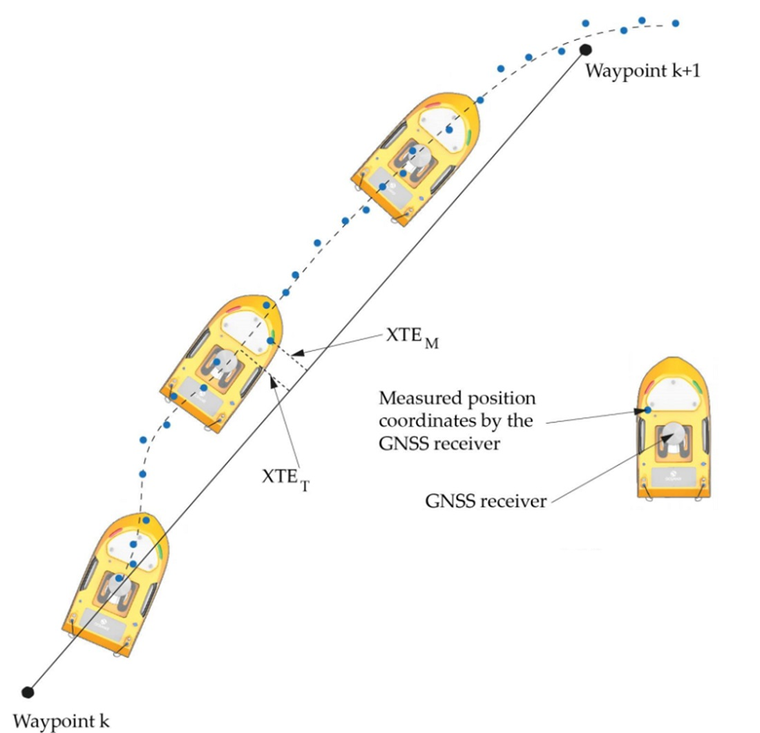
2.1. XTE Parameter of the USV

To obtain the highest possible accuracy of an USV’s path following along the profile, the vessel must navigate as close as possible to the transverse distance from the indicated path line. This is defined by the XTE parameter [45]. When executing hydrographic surveys using a manned vessel, the vessel is maintained on a path by an experienced helmsman. Moreover, the helmsman’s task is to maneuver the vessel into the next sounding profile with the smallest cross track error parameter value and the smallest yaw value of the unmanned surface vehicle (oscillating movement around the vessel’s vertical axis). Too large a deviation from the set profile may result in the need to repeat it. For USVs that perform measurements autonomously, a navigation system is responsible for maintaining the unmanned surface vehicle on the sounding profile. The control over the course and speed of the USV is executed by an autopilot, based on a PID controller. The task of proportional-integral-derivative controllers is to minimize the value of $e\left(t\right)$ error in the function of time through the control and verification of the $u\left(t\right)$ variable. The $e\left(t\right)$ error value is the difference between the expected value of $r\left(t\right)$ and a measured (actual) value of $y\left(t\right)\left[e\left(t\right)=r\left(t\right)-y\left(t\right)\right]$. This variable is represented by the controlled value (e.g., actual course or actual speed). The formula for the PID controller is [41]:

$$u\left(t\right)=A\cdot e\left(t\right)+\frac{1}{B}{\displaystyle \underset{0}{\overset{t}{\int }}e\left(t\right)}dt+C\cdot \frac{de\left(t\right)}{dt}$$

(2)

The tuning of $A$, $B$ and $C$ coefficients is effected automatically [46,47,48] or manually [49] during sea trials. They pertain, respectively, to the amplification of proportional, integral and derivative terms. The autopilot steering function $u\left(t\right)$ should influence the vessel’s rudder displacement or control of pump-jets’ momentum (depending on the USV’s construction) so that the difference between the set value and the actual course and speed would approach 0. An unmanned surface vehicle that conducts a mission autonomously should be navigated in a way that makes it possible to reach the next waypoint in the shortest time possible. But this approach differs from the approach required in hydrographic surveys, which consists of the fact that the USV should navigate as close as possible to the planned sounding profile. For this to be possible, the measured value of the XTE parameter should be minimized, meaning the sum of the actual cross track error parameter value and the projection of the position error is determined by the GNSS receiver on the perpendicular to the USV’s track (Figure 1):

$$XT{E}_M=XT{E}_T+{\delta }_{GNSS}$$

(3)

where:

$XT{E}_M$—measured value of the XTE parameter;

$XT{E}_T$—actual value of the XTE parameter;

${\delta }_{GNSS}$—projection of the position error determined by the GNSS receiver on the perpendicular to the USV’s track.

For the measurement of the XTE parameter to be as close as possible to the actual value, the positioning system should be used with the best possible operational and technical characteristics. Therefore, the maneuvering tests of an USV were performed using a geodetic GNSS RTK receiver, whose positioning accuracy amounts to 2–5 cm (p = 0.95).

2.2. Measurements

The research was conducted at a reservoir located at Wileńska Street in Gdańsk (Figure 2). They were made during favorable hydrometeorological conditions, i.e., when there were no sea currents or wind waves [50]. In this study, an USV equipped with a GNSS RTK receiver (positioning accuracy: 1–2 cm, p = 0.95) was used and tasked with navigating autonomously along the pre-planned four test routes. For the first two of them, the sounding profiles were located parallel to each other, and the distance between the lines was 5 m (Figure 2b) or 10 m (Figure 2a). However, the other two routes resembled the shape of “narrowing squares” towards the center of the waterbody being sounded. In these cases, it was decided to assume that the distance between the successive polygons will amount to 5 m (Figure 2d) and 10 m (Figure 2c).

The measurement platform used for the research was an OceanAlpha USV SL20 (OceanAlpha Group Ltd., Hong Kong, China) in an autonomous version (Figure 3). The undeniable advantages of the unmanned surface vehicle, which were a decisive factor in its selection, are small size and high maneuverability, allowing it to navigate over tight routes. Moreover, another advantage of the USV is the pump-jet propulsion, which renders it possible to navigate the vessel in waterbodies overgrown with aquatic vegetation, e.g., reeds. For measurement equipment, the unmanned surface vehicle was navigated along the profiles with a geodetic Leica Viva GNSS GS15 receiver (Leica Geosystems, St. Gallen, Switzerland), which registered National Marine Electronics Association (NMEA) GGA messages with a frequency of 5 Hz, as well as a three-axis magnetic compass with a Micro-Electro-Mechanical Systems (MEMS) three-axis accelerometer and a Honeywell HMC6343 (Honeywell Aerospace, Phoenix, AZ, USA), which is characterized by an average course measurement error of 2 m (p = 0.68). The technical specification of the USV is presented in

Table 1. Technical specification of the OceanAlpha USV SL20.

Parameter	OceanAlpha USV SL20
Hull material	Carbon fiber
Dimension	105 cm × 55 cm × 35 cm
Weight	17 kg
Payload	8 kg
Draft	15 cm
Propulsion	water-jet propulsion
Communication range	Autopilot: 2 kmRemote Control: 1 km
Remote control frequency	900 MHz/2.4 GHz
Data telemetry frequency	2.4 GHz/5.8 GHz
Survey speed	2–5 kn (1–2.5 m/s)
Max speed	10 kn (5 m/s)
Battery	6 h (1.5 m/s), 1 × 33 V 40 Ah
Positioning (standard—not used)	u-blox LEA-6 series
Positioning (used in maneuvering)	Leica Viva GNSS GS15 receiver
Heading	Honeywell HMC6343
Echosounder	Echologger series SBES

. Due to the good hydrometeorological conditions, the autopilot coefficients were as follows: $A=0.9$, $\frac{1}{B}=0.05$ and $C=0.05$. The autopilot frequency was set to 5 Hz. These are the factory defaults for this unmanned surface vehicle.

For the purpose of planning the sounding profiles, HYPACK 2020 software (HYPACK, Middletown, CT, USA) was used (Figure 4a). Following the planning, they were exported into files (in *.l84 format) containing coordinates of the waypoints of individual routes. This format is supported by the software of the USV (Figure 4b) and, owing to this, the sounding profiles could be imported into the measurement campaign schedule. The maneuvering tests for individual routes were carried out with three different power settings of the pump-jet (20%, 60% and 90%). The above settings submitted to average speeds of the vessel, amounting to, respectively, approx. 1.25 kn, 2.5 kn and 5 kn. Varied parameters of the pump-jet’s power allowed for testing the maneuverability of the unmanned surface vehicle in water with various test speeds. Following the import of the measurement campaign schedule into BaseStation 1.5 software (OceanAlpha Group Ltd., Hong Kong, China), the USV started to maneuver with a set speed over a straight line towards the first waypoint of the route. After the end of a mission (following all sounding profiles), the unmanned surface vehicle stopped after navigating through the last waypoint of the route. Over the course of the mission execution, it was noted that the USV had difficulty navigating to the last sounding profile (profile 11 for routes No. 1 and 3 or profile 21 for routes No. 2 and 4) due to the presence of dense aquatic vegetation along the shoreline of the tested waterbody.

2.3. Algorithm for Determining the XTE Parameter

In order to evaluate the USV’s maneuvering capabilities, the authors elaborated an algorithm for determining the XTE parameter. To calculate the distance between the planned routes and ways travelled by the unmanned surface vehicle, each route had to be described mathematically. In connection with the above, it was assumed that there is a given set containing $n$ coordinate vectors of subsequent waypoints (expressed in a rectangular coordinate system) $\mathbb{Z}=\left[\left(X_{WPT\left(1\right)},Y_{WPT\left(1\right)}\right),\left(X_{WPT\left(2\right)},Y_{WPT\left(2\right)}\right)\dots \left(X_{WPT\left(n\right)},Y_{WPT\left(n\right)}\right)\right]$ and a set containing $m$ coordinate vectors measured when an USV navigating along sounding profiles (expressed in a rectangular coordinate system) $ℝ=\left[\left(X_{USV\left(1\right)},Y_{USV\left(1\right)}\right),\left(X_{USV\left(2\right)},Y_{USV\left(2\right)}\right)\dots \left(X_{USV\left(m\right)},Y_{USV\left(m\right)}\right)\right]$ Assuming that ${\left[\begin{array}{cc}{X}_{WPT\left(i\right)}& Y_{WPT\left(i\right)}\end{array}\right]}^T,{\left[\begin{array}{cc}{X}_{WPT\left(i+1\right)}& Y_{WPT\left(i+1\right)}\end{array}\right]}^T$ are vectors containing subsequent route waypoints, then j-th straight line running through them will have the following form:

$$F_j=\left(y-Y_{WPT\left(i\right)}\right)\cdot \left(X_{WPT\left(i+1\right)}-X_{WPT\left(i\right)}\right)-\left(x-X_{WPT\left(i\right)}\right)\cdot \left(Y_{WPT\left(i+1\right)}-Y_{WPT\left(i\right)}\right)$$

(4)

From the given general form linear equation, one may determine a slope for j-th straight line $\left(a_j\right)$ using the following formula:

$$a_j=\frac{Y_{WPT\left(i+1\right)}-Y_{WPT\left(i\right)}}{X_{WPT\left(i+1\right)}-X_{WPT\left(i\right)}}$$

(5)

$b_j$ is a y-intercept for j-th straight line, defined as follows:

$$b_j=\frac{Y_{WPT\left(i\right)}\cdot X_{WPT\left(i+1\right)}-Y_{WPT\left(i+1\right)}\cdot X_{WPT\left(i\right)}}{X_{WPT\left(i+1\right)}-X_{WPT\left(i\right)}}$$

(6)

The subsequent steps of determining the XTE_M parameter are presented in an algorithm (Figure 5).

The algorithm requires some explanation. It consists of three main loops. The first loop (lines 1–15) segregates the profile coordinates. The minimum and maximum coordinates from the individual sounding profile (numerical value of the coordinate) are selected. The coordinates segregated at this stage will be used in the subsequent stages of the algorithm (in the if loop from line 19 to 21). The next step is to determine a point, $P_{line}\left(X_{line},Y_{line}\right)$, which lies within the given hydrographic profile and is found the closest to the position measured by the USV $P_{WPT}\left(X_{WPT\left(i\right)},Y_{WPT\left(i\right)}\right)$ (line 18). This step is needed to check if the unmanned surface vehicle is following or has gone beyond the sounding profile. Therefore, the algorithm then verifies whether a given point, $P_{line}\left(X_{line},Y_{line}\right)$, lies within the profile that is limited by the point $P_{WPT\min }\left(X_{WPTj\min },Y_{WPTj\min }\right)$ and $P_{WPT\max }\left(X_{WPTj\max },Y_{WPTj\max }\right)$ (lines 19–21). If this condition is met, the value of the $XT{E}_{Mi}$ parameter value will be determined (line 23); otherwise, if this criterion is not met, $XT{E}_{Mi}$ is assigned an infinitely large numeric value (line 26). The operation in lines 16–29 is repeated for all coordinate vectors registered by the USV and for each of the route profiles. For the position of coordinates that were not assigned to a point on the hydrographic profile (due to its presence outside the indicated range of coordinates that was determined in the if loop from line 19 to 21), the algorithm (line 30–39) determines the closest waypoint of the route and then calculates the Euclidean distance to this point—$XT{E}_{Mi}$ (so the infinitely large numerical value is to be replaced by the real value representing distance to the closest waypoint from the whole waypoint set). The principle of XTE determination is illustrated in Figure 6.

3. Results

Following the calculation of the distance between the planned routes and the ways travelled by the USV, it was possible to conduct a statistical analysis of this variable [4,51]. As an evaluation criterion, two accuracy measures were adopted: XTE68 and XTE95. These measures describe what value is not exceeded by, respectively, 68% (XTE68) and 95% (XTE95) of the distance in two-dimensional space (2D), calculated based on points registered by the RTK receiver and points belonging to the route. In

Table 2. Cross track error (XTE) measures of steering an Unmanned Surface Vehicle (USV), travelling at a speed of 1.25 kn for individual routes.

Accuracy Measure	Route No. 1	Route No. 2	Route No. 3	Route No. 4
Number of measurements	571	1 092	542	905
XTE68	2.11 m	1.73 m	1.46 m	1.62 m
XTE95	2.72 m	2.36 m	2.13 m	2.32 m

,

Table 3. Cross track error (XTE) measures of steering an Unmanned Surface Vehicle (USV), travelling at a speed of 2.5 kn for individual routes.

Accuracy Measure	Route No. 1	Route No. 2	Route No. 3	Route No. 4
Number of measurements	262	440	249	435
XTE68	1.43 m	1.31 m	1.00 m	1.16 m
XTE95	1.99 m	1.85 m	2.42 m	2.28 m

and

Table 4. Cross track error (XTE) measures of steering an Unmanned Surface Vehicle (USV), travelling at a speed of 5 kn for individual routes.

Accuracy Measure	Route No. 1	Route No. 2	Route No. 3	Route No. 4
Number of measurements	159	286	160	281
XTE68	1.85 m	1.57 m	2.18 m	1.92 m
XTE95	2.74 m	2.44 m	2.76 m	2.40 m

, there are values presented for XTE68 and XTE95 measurements, which were determined based on the real time kinematic receiver’s indications for individual routes.

Table 2 shows that the accuracy of the USV’s maintenance along the profile was not influenced by the route shape or the distance between the lines. The value of the XTE68 measurement oscillated in the range of 1.5–2 m, and the XTE95 error was slightly larger and amounted to approx. 2–2.5 m. The small differences between the obtained values of XTE measures were definitely influenced by the Horizontal Dilution of Precision (HDOP) that was used to determine 2D position coordinates. However, its value oscillated in the range of 0.7–0.9 for individual routes (Figure 7) which, according to other studies [52,53], may be considered to be perfect satellite signal quality.

To verify the repeatability of measurements, the USV’s maneuvering tests were re-conducted with higher speeds (Table 3 and Table 4).

The next measurement series was executed with double the test speed (2.5 kn). As shown in Table 3, the obtained values of XTE measures are better (by approx. 50 cm) than the values obtained in the first measurement series. This is particularly true for XTE68 measures which reach an approximate value of 1–1.5 m. It should be stressed that, again, smaller errors (by a dozen or so centimeters) in USV navigation were obtained for routes with smaller mutual distances between sounding profiles (route No. 2 and 4). The conditions for execution of GNSS satellite measurements also proved to be similar to the first measurement series (HDOP: 0.7–0.9, number of visible satellites: 12–16).

Moreover, the maneuvering tests were also conducted at the highest possible test speed, as declared by the manufacturer (5 kn). Table 4 shows that the accuracy of the path following the USV along the profile is almost identical with the slowest (1.25 kn), as well as the fastest (5 kn) speed. The value of the XTE68 measure reached the range of 1.5–2 m, while the XTE95 error was slightly larger (2.5 m).

In the subsequent phase, the USV’s trajectory was illustrated with XTE error values plotted in relation to the planned routes. As shown in Figure 8b, the average cross track error measure was the smallest (1.05 m) during navigation over route No. 1, with an average test speed. On the other hand, the worst accuracy of the USV’s path following along the profile (1.63 m) was obtained during maneuvering tests carried out with the lowest speed. It should be stressed that the average XTE error was similar to runs with the average and the highest test speeds (the difference between them amounted to a dozen or so centimeters).

Next, the influence of the value of XTE error in the function of the length of the travelled route was evaluated. In the diagrams shown in Figure 9, the waypoints of the route are also added, owing to which it was possible to determine the accuracy of the USV’s path following the profile, both over straight sections as well as curves. Figure 9 shows that the values of the cross track error were smaller when travelling around turns (< 1 m) than when the unmanned surface vehicle moved in straight sections (approx. 2 m). It is worth stressing that when the USV travelled with the highest test speed, the variability of the XTE error was the highest. For example, the analyzed accuracy measure varied regularly over every second straight section. In profiles No. 1, 5 and 9 it reached the value of approx. 2 m, and in other profiles (sounding lines No. 3, 7 and 11) it did not exceed 0.5 m.

In comparison to route No. 1, way No. 2 was only half the distance between the sounding profiles (5 m). In Figure 10, an identical tendency as in Figure 8 was observed. Again, the smallest average value of XTE error was obtained during a run with an average test speed (0.92 m), and the worst accuracy of the USV’s path following along the profile (1.34 m) was obtained for the slowest speed. It is interesting that although route No. 2 was more spiral than way No. 1, the average values of cross track errors were smaller by approx. 10–30 cm for individual speeds.

As seen in Figure 11, when travelling the USV over route No. 2 with the average and the highest test speeds, the XTE error values varied alternately along individual straight sections. For some sounding profiles, it oscillated around 0.5 m, and for the remaining hydrographic profiles it reached the range of 2–2.5 m. Moreover, there was no increase in XTE measures over turns for all the speeds observed.

Subsequently, routes No. 3 and 4 were subject to analysis, whose shape resembled “narrowing squares”. Figure 12 shows that the values of the average XTE error are almost identical for various test speeds (they differ about 20 cm) and reach approx. 1 m. The accuracy of the USV’s path following the profile on route No. 3 is similar to the accuracies obtained on ways No. 1 and 2, which feature a different layout of sounding profiles (parallel). Despite the change in the layout of sounding profiles, the lowest average cross track error (0.95 m) was—again, as in the case of routes No. 1 and 2—obtained for the average speed.

In Figure 13, there is a large variability of XTE error visible, irrespective of the test speed. For approx. half of the sounding profiles, the analyzed measure reaches the range of 0.5–1 m, and for the rest of the profiles, the accuracy of the USV’s path following along the profile is half as much and amounts to 1.5–2 m.

Route No. 4 differed from way No. 3 with mutual distances between sounding profiles and the value amounting to 5 m instead of 10 m. When travelling turns of the last route, almost identical values of an average XTE error were obtained, both for route No. 3, as well as for sounding profiles in a parallel layout. The accuracy of the USV’s path following the profile oscillated at 1 m, irrespective of the test speed (Figure 14).

As in the case of routes No. 1, 2 and 3, the value of XTE error reached the range of 0.5–2 m. For example, for route No. 4, which was travelled with the highest test speed, it was observed that, on average, the cross track error changed its value from 1 m to 2 m and vice versa every two sounding profiles (Figure 15c).

4. Discussion

Identical measurements (over the same routes) were carried out on 7 March 2019 using an USV of HyDrone, which was navigated in an autonomous mode using a popular autopilot (Pixhawk) and a Global Positioning System (GPS)/GLObal NAvigation Satellite System (GLONASS) u-blox NEO-M8N receiver (u-blox, Thalwil, Switzerland) supported with a Fluxgate magnetic compass [4]. The 2019 maneuvering tests were carried out for one test speed, which was similar to the lowest speed during the 2020 measurements (1.25 kn). Therefore, a comparative analysis was conducted of the obtained values of XTE measures over the 2019 and 2020 measurement campaigns (

Table 5. Accuracy measures following an USV’s path, travelling at a speed of 1.25 kn for individual routes during the 2019 and 2020 measurement campaigns.

Accuracy Measure	Route No. 1	Route No. 2	Route No. 3	Route No. 4
Measurement year	2019	2020	2019	2020
Number of measurements	458	571	848	1 092
XTE68	0.92 m	2.11 m	1.15 m	1.73 m
XTE95	2.01 m	2.72 m	2.38 m	2.36 m

).

In order to determine the changes in the value of XTE measures between the first and the second measurement campaigns, it was decided to assume a relative percentage change of these measures using the following formulas [4,51]:

$$\Delta XTE68=\frac{XTE{68}_{2019,k}-XTE{68}_{2020,k}}{XTE{68}_{2019,k}}\cdot 100\%$$

(7)

where:

$XTE{68}_{2019,k}$—XTE68 measure value for k-th route during the 2019 measurement campaign [m];

$XTE{68}_{2020,k}$—XTE68 measure value for k-th route during the 2020 measurement campaign [m];

$k$—route number;

and:

$$\Delta XTE95=\frac{XTE{95}_{2019,k}-XTE{95}_{2020,k}}{XTE{95}_{2019,k}}\cdot 100\%$$

(8)

where:

$XTE{95}_{2019,k}$—XTE95 measure value for k-th route during the 2019 measurement campaign [m];

$XTE{95}_{2020,k}$—XTE95 measure value for k-th route during the 2020 measurement campaign [m].

Figure 16 shows that the values of XTE68 and XTE95 measures obtained during the 2019 and 2020 measurement campaigns are similar. For example, the value of the XTE95 error for routes No. 2, 3 and 4 differed between each other by a few centimeters (the relative percentage change of XTE95 measures reaches approx. 1–3%). A greater change in the value of the XTE95 measure was found for route No. 1 and it amounted to approx. 70 cm. Therefore, it may be stated that XTE95 errors oscillated in the range of 2–2.5 m. For the XTE68 measure, it was approx. twice as low as the XTE95 measure and amounted to 1–1.5 m. However, relative percentage changes of the XTE68 error for individual routes in the 2019 and 2020 measurement campaigns were larger than in the case of XTE95 measure. For example, the accuracy of the USV’s path following along routes No. 2, 3 and 4 differed by only a few centimeters to approx. 50 cm (the relative percentage change of XTE68 measures reaches approx. 4–50%). A greater change in the value of the XTE68 measure was found for route No. 1 and it exceeded 1 m.

Undoubtedly, the following elements influence the accuracy of the USV’s path following along a profile: the positioning system used for navigation and the magnetic compass used for maintaining the course of an USV. During the 2019 and 2020 measurement campaigns, devices with varied operational and technical characteristics were used. Over the first campaign, a GPS/GLONASS u-blox NEO-M8N receiver was used, supported by a Fluxgate magnetic compass. It should be noted that the manufacturer of the receiver did not provide information on the receiver’s measurement accuracy with the GPS/GLONASS method and defined it only for each system separately. Using GPS satellites, positioning accuracy is provided in the range of 2–2.5 m Circular Error Probable (CEP), while with the use of GLONASS satellites, the accuracy amounts to 4 m in the horizontal plane (the manufacturer did not provide information about a possible position error for the given value). However, the magnetic compass features a high course measurement accuracy of 0.3° (p = 0.50 at 30 m/s), as opposed to other popularly used devices for determining the course of a vessel. For example, satellite compasses and gyrocompass devices usually determine the course with an accuracy of 1°–1.5° [54]. Nevertheless, under unfavorable conditions, their accuracy can drop to 10° [55,56]. With respect to the 2020 measurement campaign, and in comparison with the 2019 measurement campaign, a geodetic GNSS receiver was used, allowing for executing measurements in real-time with a centimeter-level accuracy [57,58]. Whereas the magnetic compass used in the OceanAlpha USV SL20 featured a high stability of course maintenance of 1°–3° RMS. This resulted in the accuracy values of the USV’s navigation along a profile being similar to those obtained using a multi-GNSS receiver, supported with a Fluxgate magnetic compass. Based on email communication with one of Oceanalpha’s representatives, it was learned that the results obtained during the 2020 measurement campaign were similar to the declared ones. However, the manufacturer of the OceanAlpha USV SL20 recommends that in order to obtain a smaller value of the XTE error (in the range of 0.3–1 m or less), a stable magnetic compass should be used or an Inertial Navigation System (INS) with a double-antenna solution, e.g., VectorNav VN-300 [59].

5. Conclusions

This study found that an USV operating in autonomous mode with the use of autopilot and a RTK receiver (positioning accuracy: 1–2 cm, p = 0.95), supported by a magnetic compass (course measurement accuracy: 1°–3°, p = 0.50 at 30 m/s), provides for effective execution of bathymetric measurements, especially in small, ultra-shallow inland waterbodies. The analyzed solution makes it possible to maintain the vessel on sounding profiles with an accuracy of 1.46–2.11 m (p = 0.68) and 2.13–2.72 m (p = 0.95). Thus, it meets the requirements of the IHO order 2 [16] for hydrographic system positioning accuracy. Additionally, it needs to be stressed that the accuracy of the unmanned surface vehicle’s path following along the profile was not influenced by the speed of the USV (1.25 kn, 2.5 kn and 5 kn), the route shape (parallel sounding lines and “narrowing squares”) or the distance between the profiles (5 m and 10 m).

The authors of the paper are planning to execute maneuvering tests of the USV using a RTK receiver, supported with a precise magnetic compass (course measurement accuracy: 0.1°) and with the use of an INS, employing a double-antenna solution. It is expected that the obtained unmanned surface vehicle navigation accuracy along profiles will be in the range of several dozen centimeters.

References

1. Brčić, D.; Kos, S.; Žuškin, S. Navigation with ECDIS: Choosing the Proper Secondary Positioning Source. TransNav Int. J. Mar. Navig. Saf. Sea Transp. 2015, 9, 317–326. [Google Scholar] [CrossRef]
2. International Hydrographic Organization. Hydrographic Dictionary, 5th ed.; English Special Publication No. 32; IHO: Monte Carlo, Monaco, 1994. [Google Scholar]
3. Genchi, S.A.; Vitale, A.J.; Perillo, G.M.E.; Seitz, C.; Delrieux, C.A. Mapping Topobathymetry in a Shallow Tidal Environment Using Low-cost Technology. Remote Sens. 2020, 12, 1394. [Google Scholar] [CrossRef]
4. Specht, M.; Specht, C.; Lasota, H.; Cywiński, P. Assessment of the Steering Precision of a Hydrographic Unmanned Surface Vessel (USV) along Sounding Profiles Using a Low-cost Multi-Global Navigation Satellite System (GNSS) Receiver Supported Autopilot. Sensors 2019, 19, 3939. [Google Scholar] [CrossRef] [PubMed] [Green Version]
5. Specht, C.; Specht, M.; Cywiński, P.; Skóra, M.; Marchel, Ł.; Szychowski, P. A New Method for Determining the Territorial Sea Baseline Using an Unmanned, Hydrographic Surface Vessel. J. Coast. Res. 2019, 35, 925–936. [Google Scholar] [CrossRef]
6. Umbach, M.J. Hydrographic Manual, 4th ed.; NOAA: Silver Spring, MD, USA, 1976. [Google Scholar]
7. United States Army Corps of Engineers. EM 1110-2-1003 USACE Standards for Hydrographic Surveys; USACE: Washington, DC, USA, 2013. [Google Scholar]
8. Grządziel, A.; Felski, A.; Wąż, M. Experience with the Use of a Rigidly-mounted Side-scan Sonar in a Harbour Basin Bottom Investigation. Ocean Eng. 2015, 109, 439–443. [Google Scholar] [CrossRef]
9. Jang, W.; Park, H.; Park, S. Analysis of Positioning Accuracy of PPP, VRS, DGPS in Coast and Inland Water Area of South Korea. J. Coast. Res. 2018, 85, 1276–1280. [Google Scholar] [CrossRef]
10. Jang, W.; Park, H.; Seo, K.; Kim, Y. Analysis of Positioning Accuracy Using Differential GNSS in the Coast and Port Area of South Korea. J. Coast. Res. 2016, 75, 1337–1341. [Google Scholar] [CrossRef]
11. Song, F.; Gong, S.; Zhou, R. Underwater Topography Survey and Precision Analysis Based on Depth Sounder and CORS-RTK Technology. IOP Mater. Sci. Eng. 2020, 780, 042051. [Google Scholar] [CrossRef]
12. Baptista, P.; Bastos, L.; Bernardes, C.; Cunha, T.; Dias, J. Monitoring Sandy Shores Morphologies by DGPS–A Practical Tool to Generate Digital Elevation Models. J. Coast. Res. 2008, 246, 1516–1528. [Google Scholar] [CrossRef]
13. Dziewicki, M.; Specht, C. Position Accuracy Evaluation of the Modernized Polish DGPS. Pol. Marit. Res. 2009, 16, 57–61. [Google Scholar] [CrossRef]
14. Moore, T.; Hill, C.; Monteiro, L. Is DGPS Still a Good Option for Mariners? J. Navig. 2001, 54, 437–446. [Google Scholar] [CrossRef]
15. Szot, T.; Specht, C.; Specht, M.; Dabrowski, P.S. Comparative Analysis of Positioning Accuracy of Samsung Galaxy Smartphones in Stationary Measurements. PLoS ONE 2019, 14, e0215562. [Google Scholar] [CrossRef] [PubMed]
16. Canadian Hydrographic Service. CHS Standards for Hydrographic Surveys, 2nd ed.; CHS: Ottawa, ON, Canada, 2013. [Google Scholar]
17. International Hydrographic Organization. IHO Standards for Hydrographic Surveys, 5th ed.; Special Publication No. 44; IHO: Monte Carlo, Monaco, 2008. [Google Scholar]
18. International Hydrographic Organization. Manual on Hydrography, 1st ed.; Publication C-13; IHO: Monte Carlo, Monaco, 2005. [Google Scholar]
19. National Oceanic and Atmospheric Administration. NOS Hydrographic Surveys Specifications and Deliverables; NOAA: Silver Spring, MD, USA, 2017. [Google Scholar]
20. Breivik, M. Topics in Guided Motion Control of Marine Vehicles. Ph.D. Thesis, Norwegian University of Science and Technology, Trondheim, Norway, 2010. [Google Scholar]
21. Liu, Z.; Zhang, Y.; Yu, X.; Yuan, C. Unmanned Surface Vehicles: An Overview of Developments and Challenges. Ann. Rev. Control 2016, 41, 71–93. [Google Scholar] [CrossRef]
22. Kum, B.-C.; Shin, D.-H.; Lee, J.H.; Moh, T.J.; Jang, S.; Lee, S.Y.; Cho, J.H. Monitoring Applications for Multifunctional Unmanned Surface Vehicles in Marine Coastal Environments. J. Coast. Res. 2018, 85, 1381–1385. [Google Scholar] [CrossRef]
23. Bellingham, J.G.; Rajan, K. Robotics in Remote and Hostile Environments. Science 2007, 318, 1098–1102. [Google Scholar] [CrossRef] [Green Version]
24. Specht, M.; Specht, C.; Szafran, M.; Makar, A.; Dąbrowski, P.; Lasota, H.; Cywiński, P. The Use of USV to Develop Navigational and Bathymetric Charts of Yacht Ports on the Example of National Sailing Centre in Gdańsk. Remote Sens. 2020, 12, 2585. [Google Scholar] [CrossRef]
25. Zwolak, K.; Wigley, R.; Bohan, A.; Zarayskaya, Y.; Bazhenova, E.; Dorshow, W.; Sumiyoshi, M.; Sattiabaruth, S.; Roperez, J.; Proctor, A.; et al. The Autonomous Underwater Vehicle Integrated with the Unmanned Surface Vessel Mapping the Southern Ionian Sea. The Winning Technology Solution of the Shell Ocean Discovery XPRIZE. Remote Sens. 2020, 12, 1344. [Google Scholar] [CrossRef] [Green Version]
26. Jorge, V.A.M.; Granada, R.; Maidana, R.G.; Jurak, D.A.; Heck, G.; Negreiros, A.P.F.; dos Santos, D.H.; Gonçalves, L.M.G.; Amory, A.M. A Survey on Unmanned Surface Vehicles for Disaster Robotics: Main Challenges and Directions. Sensors 2019, 19, 702. [Google Scholar] [CrossRef] [Green Version]
27. Cui, K.; Lin, B.; Sun, W.; Sun, W. Learning-based Task Offloading for Marine Fog-cloud Computing Networks of USV Cluster. Electronics 2019, 8, 1287. [Google Scholar] [CrossRef] [Green Version]
28. Naus, K.; Marchel, Ł. Use of a Weighted ICP Algorithm to Precisely Determine USV Movement Parameters. Appl. Sci. 2019, 9, 3530. [Google Scholar] [CrossRef] [Green Version]
29. Stateczny, A.; Kazimierski, W.; Burdziakowski, P.; Motyl, W.; Wisniewska, M. Shore Construction Detection by Automotive Radar for the Needs of Autonomous Surface Vehicle Navigation. ISPRS Int. J. Geo-Inf. 2019, 8, 80. [Google Scholar] [CrossRef] [Green Version]
30. Lv, C.; Yu, H.; Hua, Z.; Li, L.; Chi, J. Speed and Heading Control of an Unmanned Surface Vehicle Based on State Error PCH Principle. Math. Probl. Eng. 2018, 2018, 7371829. [Google Scholar] [CrossRef] [Green Version]
31. Wang, L.; Wu, Q.; Liu, J.; Li, S.; Negenborn, R.R. State-of-the-art Research on Motion Control of Maritime Autonomous Surface Ships. J. Mar. Sci. Eng. 2019, 7, 438. [Google Scholar] [CrossRef] [Green Version]
32. Cho, H.; Jeong, S.-K.; Ji, D.-H.; Tran, N.-H.; Vu, M.T.; Choi, H.-S. Study on Control System of Integrated Unmanned Surface Vehicle and Underwater Vehicle. Sensors 2020, 20, 2633. [Google Scholar] [CrossRef] [PubMed]
33. Mou, J.; He, Y.; Zhang, B.; Li, S.; Xiong, Y. Path Following of a Water-jetted USV Based on Maneuverability Tests. J. Mar. Sci. Eng. 2020, 8, 354. [Google Scholar] [CrossRef]
34. Giordano, F.; Mattei, G.; Parente, C.; Peluso, F.; Santamaria, R. Integrating Sensors into a Marine Drone for Bathymetric 3D Surveys in Shallow Waters. Sensors 2016, 16, 41. [Google Scholar] [CrossRef] [PubMed] [Green Version]
35. Suhari, K.T.; Karim, H.; Gunawan, P.H.; Purwanto, H. Small ROV Marine Boat for Bathymetry Surveys of Shallow Waters—Potential Implementation in Malaysia. Int. Arch. Photogramm. Remote. Sens. Spat. Inf. Sci. 2017, XLII-4/W5, 201–208. [Google Scholar] [CrossRef] [Green Version]
36. Mattei, G.; Troisi, S.; Aucelli, P.P.C.; Pappone, G.; Peluso, F.; Stefanile, M. Sensing the Submerged Landscape of Nisida Roman Harbour in the Gulf of Naples from Integrated Measurements on a USV. Water 2018, 10, 1686. [Google Scholar] [CrossRef] [Green Version]
37. Cloet, R.L. The Effect of Line Spacing on Survey Accuracy in a Sand-wave Area. Hydrogr. J. 1976, 2, 5–11. [Google Scholar]
38. Bouwmeester, E.C.; Heemink, A.W. Optimal Line Spacing in Hydrographic Survey. Int. Hydrogr. Rev. 1993, LXX, 37–48. [Google Scholar]
39. Yang, Y.; Li, Q.; Zhang, J.; Xie, Y. Iterative Learning-based Path and Speed Profile Optimization for an Unmanned Surface Vehicle. Sensors 2020, 20, 439. [Google Scholar] [CrossRef] [PubMed] [Green Version]
40. Kadyrov, M.; Greshnikov, P.; Maltsev, S.; Maistro, A.; Pereverzev, A.; Kiselev, K.; Durnev, A.; Starobinskii, E.; Buldakov, P. Design and Construction of the Cadet-M Unmanned Marine Platform Using Alternative Energy. E3S Web Conf. 2019, 140, 02011. [Google Scholar] [CrossRef] [Green Version]
41. Stateczny, A.; Burdziakowski, P.; Najdecka, K.; Domagalska-Stateczna, B. Accuracy of Trajectory Tracking Based on Nonlinear Guidance Logic for Hydrographic Unmanned Surface Vessels. Sensors 2020, 20, 832. [Google Scholar] [CrossRef] [PubMed] [Green Version]
42. Aguiar, A.P.; Hespanha, J.P. Trajectory-tracking and Path following of Underactuated Autonomous Vehicles with Parametric Modeling Uncertainty. IEEE Trans. Autom. Control 2007, 52, 1362–1379. [Google Scholar] [CrossRef] [Green Version]
43. Do, K.D.; Pan, J. Global Tracking Control of Underactuated Ships with Nonzero Off-diagonal Terms in Their System Matrices. Automatica 2005, 41, 87–95. [Google Scholar] [CrossRef]
44. Li, C.; Jiang, J.; Duan, F.; Liu, W.; Wang, X.; Bu, L.; Sun, Z.; Yang, G. Modeling and Experimental Testing of an Unmanned Surface Vehicle with Rudderless Double Thrusters. Sensors 2019, 19, 2051. [Google Scholar] [CrossRef] [Green Version]
45. Kristić, M.; Žuškin, S.; Brčić, D.; Valčić, S. Zone of Confidence Impact on Cross Track Limit Determination in ECDIS Passage Planning. J. Mar. Sci. Eng. 2020, 8, 566. [Google Scholar] [CrossRef]
46. Azar, A.T.; Ammar, H.H.; Ibrahim, Z.F.; Ibrahim, H.A.; Mohamed, N.A.; Taha, M.A. Implementation of PID Controller with PSO Tuning for Autonomous Vehicle. In Proceedings of the International Conference on Advanced Intelligent Systems and Informatics 2019 (AISI 2019), Cairo, Egypt, 26–28 October 2019. [Google Scholar]
47. Miskovic, N.; Vukic, Z.; Barisic, M.; Tovornik, B. Autotuning Autopilots for Micro-ROVs. In Proceedings of the 2006 14th Mediterranean Conference on Control and Automation (MED 2006), Ancona, Italy, 28–30 June 2006. [Google Scholar]
48. Pan, Y.; Huang, D.; Sun, Z. Backstepping Adaptive Fuzzy Control for Track-keeping of Underactuated Surface Vessels. Control Theory Appl. 2011, 28, 907–914. [Google Scholar]
49. Chattopadhyay, S.; Roy, G.; Panda, M. Simple Design of a PID Controller and Tuning of Its Parameters Using LabVIEW Software. Sens. Transducers 2011, 129, 69–85. [Google Scholar]
50. Specht, M.; Specht, C.; Wąż, M.; Naus, K.; Grządziel, A.; Iwen, D. Methodology for Performing Territorial Sea Baseline Measurements in Selected Waterbodies of Poland. Appl. Sci. 2019, 9, 3053. [Google Scholar] [CrossRef] [Green Version]
51. Specht, C.; Szot, T.; Dąbrowski, P.; Specht, M. Testing GNSS Receiver Accuracy in Samsung Galaxy Series Mobile Phones at a Sports Stadium. Meas. Sci. Technol. 2020, 31, 064006. [Google Scholar] [CrossRef]
52. Hasan, M.; Rouf, R.R.; Islam, S. Investigation of Most Ideal GNSS Framework (GPS, GLONASS and GALILEO) for Asia Pacific Region (Bangladesh). Int. J. Appl. Inf. Syst. 2017, 12, 33–37. [Google Scholar] [CrossRef]
53. Protaziuk, E. Geometric Aspects of Ground Augmentation of Satellite Networks for the Needs of Deformation Monitoring. Artif. Satell. 2016, 51, 75–88. [Google Scholar] [CrossRef] [Green Version]
54. Jaskólski, K.; Felski, A.; Piskur, P. The Compass Error Comparison of an Onboard Standard Gyrocompass, Fiber-Optic Gyrocompass (FOG) and Satellite Compass. Sensors 2019, 19, 1942. [Google Scholar] [CrossRef] [Green Version]
55. Dąbrowski, P.S.; Specht, C.; Felski, A.; Koc, W.; Wilk, A.; Czaplewski, K.; Karwowski, K.; Jaskólski, K.; Specht, M.; Chrostowski, P.; et al. The Accuracy of a Marine Satellite Compass under Terrestrial Urban Conditions. J. Mar. Sci. Eng. 2020, 8, 18. [Google Scholar] [CrossRef] [Green Version]
56. Felski, A. Exploitative Properties of Different Types of Satellite Compasses. Ann. Navig. 2010, 16, 33–40. [Google Scholar]
57. Siejka, Z. Validation of the Accuracy and Convergence Time of Real Time Kinematic Results Using a Single Galileo Navigation System. Sensors 2018, 18, 2412. [Google Scholar] [CrossRef] [Green Version]
58. Specht, M.; Specht, C.; Wilk, A.; Koc, W.; Smolarek, L.; Czaplewski, K.; Karwowski, K.; Dąbrowski, P.S.; Skibicki, J.; Chrostowski, P.; et al. Testing the Positioning Accuracy of GNSS Solutions during the Tramway Track Mobile Satellite Measurements in Diverse Urban Signal Reception Conditions. Energies 2020, 13, 3646. [Google Scholar] [CrossRef]
59. Specht, M.; Specht, C.; Dąbrowski, P.; Czaplewski, K.; Smolarek, L.; Lewicka, O. Road Tests of the Positioning Accuracy of INS/GNSS Systems Based on MEMS Technology for Navigating Railway Vehicles. Energies 2020, 13, 4463. [Google Scholar] [CrossRef]
Figure 1. Graphic method of conducting the Unmanned Surface Vehicle (USV) on the sounding profile using an autopilot.
Energies 13 05637 g001
Figure 2. Sounding profiles designed in two variants: parallel (a,b) and spiral (c,d).
Energies 13 05637 g002
Figure 3. Unmanned Surface Vehicle (USV) with equipment for communication, data transmission and steering.
Energies 13 05637 g003
Figure 4. HYPACK 2019 software used for exporting and planning sounding profiles (a) and BaseStation 1.5 software used for the execution of Unmanned Surface Vehicle (USV) measurements (b).
Energies 13 05637 g004
Figure 5. Algorithm for determining the XTE parameter.
Energies 13 05637 g005
Figure 6. Graphic method of determining the cross track error (XTE) in two cases: when it is not possible to draw a straight line perpendicular to the planned sounding profile (a) and it is possible to determine the perpendicular line (b).
Energies 13 05637 g006
Figure 7. The value of Horizontal Dilution of Precision (HDOP) and the number of visible satellites in the function of the length of the travelled route No. 4 with a speed of 1.25 kn.
Energies 13 05637 g007
Figure 8. Unmanned Surface Vehicle (USV) trajectory with plotted cross track error (XTE) values (color-coded) with relation to the planned route No. 1 with a speed of 1.25 kn (a), 2.5 kn (b) and 5 kn (c).
Energies 13 05637 g008
Figure 9. Cross track error (XTE) value in the function of the travelled route No. 1 with a speed of 1.25 kn (a), 2.5 kn (b) and 5 kn (c).
Energies 13 05637 g009
Figure 10. Unmanned Surface Vehicle (USV) trajectory with plotted cross track error (XTE) values (color-coded) with relation to the planned route No. 2 with a speed of 1.25 kn (a), 2.5 kn (b) and 5 kn (c).
Energies 13 05637 g010
Figure 11. Cross track error (XTE) value in the function of the travelled route No. 2 with a speed of 1.25 kn (a), 2.5 kn (b) and 5 kn (c).
Energies 13 05637 g011
Figure 12. Unmanned Surface Vehicle (USV) trajectory with plotted cross track error (XTE) values (color-coded) with relation to the planned route No. 3 with a speed of 1.25 kn (a), 2.5 kn (b) and 5 kn (c).
Energies 13 05637 g012
Figure 13. Cross track error (XTE) value in the function of the travelled route No. 3. with a speed of 1.25 kn (a), 2.5 kn (b) and 5 kn (c).
Energies 13 05637 g013
Figure 14. Unmanned Surface Vehicle (USV) trajectory with plotted cross track error (XTE) values (color-coded) with relation to the planned route No. 4 with a speed of 1.25 kn (a), 2.5 kn (b) and 5 kn (c).
Energies 13 05637 g014
Figure 15. Cross track error (XTE) value in the function of the travelled route No. 4 with a speed of 1.25 kn (a), 2.5 kn (b) and 5 kn (c).
Energies 13 05637 g015
Figure 16. Relative percentage change of XTE68 and XTE95 measures between the 2019 and 2020 measurement campaigns.
Energies 13 05637 g016