A Higher Order Mining Approach for the Analysis of Real-World Datasets ^†

Abstract

In this study, we propose a higher order mining approach that can be used for the analysis of real-world datasets. The approach can be used to monitor and identify the deviating operational behaviour of the studied phenomenon in the absence of prior knowledge about the data. The proposed approach consists of several different data analysis techniques, such as sequential pattern mining, clustering analysis, consensus clustering and the minimum spanning tree (MST). Initially, a clustering analysis is performed on the extracted patterns to model the behavioural modes of the studied phenomenon for a given time interval. The generated clustering models, which correspond to every two consecutive time intervals, can further be assessed to determine changes in the monitored behaviour. In cases in which significant differences are observed, further analysis is performed by integrating the generated models into a consensus clustering and applying an MST to identify deviating behaviours. The validity and potential of the proposed approach is demonstrated on a real-world dataset originating from a network of district heating (DH) substations. The obtained results show that our approach is capable of detecting deviating and sub-optimal behaviours of DH substations.

1. Introduction

A fault is an abnormal state within a system that may cause a failure or a malfunction. Fault detection is the identification of an unacceptable deviation of at least one feature of the system from the expected or usual behaviour [1]. The fault detection problem has been studied in different domains and belongs to a more general category of outlier (anomaly) detection. There are several factors that make outlier detection domain-specific [2,3,4,5,6], such as the nature of the data, the availability of labelled data and the constraints and requirements of the outlier detection problem. Outlier detection techniques can be classified into three groups based on the availability of the labelled data, namely supervised methods, unsupervised methods and semi-supervised methods, where the aim is to learn what is (ab)normal and only model (ab)normality [2,3,6]. In the absence of prior knowledge of data, which is often the case for many real-world datasets due to, e.g., the expensiveness of the data labelling process by domain experts, the initial assumption is that normal data represent a significant portion of the available data.

Isermann [1,7] provided a general review of fault detection and diagnosis (FDD). The main objective of an FDD system is the early detection of faults and diagnosis of their causes to reduce maintenance costs and excessive damage to other parts of the system. Katipamula and Brambley [8,9] conducted an extensive review in two parts on FDD for building systems. The authors classified FDD methods based on the availability of a priori knowledge for formulating the diagnostics and highlighted their advantages and disadvantages.

According to this classification, FDD methods can fall into two categories: model-based methods and data-driven methods. The model-based methods require a priori knowledge of the system and can use either quantitative or qualitative models. Quantitative models are sets of mathematical relationships that are mainly based on physical properties, processes or models of a system. Qualitative models, on the other hand, use qualitative knowledge; e.g., including domain experts’ experience as a set of rules to identify proper and faulty operations. Data-driven methods use historical data that originate from a system to build models; i.e., they are system-specific. These methods have become increasingly popular in recent years. Data-driven methods are easy to develop and do not require explicit knowledge of a system, making them suitable for domains with uncertainty.

In this study, we propose a data-driven approach that also relies on domain experts’ qualitative knowledge to set user-specific thresholds for identifying deviating behaviours. We show that the proposed approach is capable of revealing patterns representing the deviating behaviours of the studied phenomenon. Such deviating behaviours can arise for different reasons; in the case of district heating (DH) systems, they might be related to faulty equipment, a sudden change of outdoor temperature and/or the social behaviour of tenants. Regardless of the reasons behind these deviating behaviours, fault detection systems should be able to provide understandable reports for domain experts. The approach proposed in this study supplies the domain experts with patterns that are suitable for human inspection. In addition, the results are visualized from different points of view to provide supplementary information for the experts. The purposed approach can be applied for the analysis of streaming data scenarios with no direct access to labelled data in different application domains; e.g., it can be used to model and monitor operational behaviour and the performance of fleets of wind turbines and solar arrays.

The contributions of the proposed approach can be summarized in the following three points:

• A data model of the studied phenomenon is built, which presents its behavioural modes for a given time interval.
• The phenomenon’s behaviour is monitored by comparing the models corresponding to two consecutive time intervals.
• Deviating behaviours are analysed and identified by the integration analysis of the built models using a domain-specific threshold.

This paper extends our previous work [10]. In the current study, the data cleaning and preparation are improved by utilizing more suitable data preprocessing methods for time series data. We apply a k-nearest neighbours-based approach for the imputation of missing data, which ensures more accurate estimations by taking into consideration the structure of the data. The seasonality of the time series is adjusted using the differencing method. In addition, the raw time series (sequences of numbers) are discretized into string series using the symbolic aggregate approximation method. Furthermore, we have conducted more extensive evaluations of the proposed approach for the chosen case study by considering a larger number of DH substations from different heat load categories. Finally, a more general explanation of the proposed approach is provided to demonstrate its applicability for similar problems in other application domains.

2. Related Work

The validity and potential of the proposed approach have been demonstrated in a use case from the DH domain. Therefore, in this section, we mainly review the literature related to outlier and fault detection approaches applied to the DH and smart buildings domains.

Fontes and Pereira [11] proposed a fault detection method for gas turbines using pattern recognition in multivariate time series. In another study [12], the authors proposed a general methodology for identifying faults based on time-series models and statistical process control, where faults can be identified as anomalies in the temporal residual signals obtained from the models using statistical process control charts.

In a recent review, Djenouri et al. [13] focused on the usage of machine learning for smart building applications. The authors classified the existing solutions into two main categories: (1) occupancy monitoring and (2) energy/device-centric approaches. These categories are further divided into a number of sub-categories where the classified solutions in each group are discussed and compared.

Gadd and Werner [14] showed that hourly meter readings can be used to detect faults at DH substations. The authors identified three fault groups: (1) low average annual temperature differences, (2) poor substation control and (3) unsuitable heat load patterns. The results of the study showed that low average annual temperature differences are the most important issues, and that addressing them can improve the efficiency of DH systems. However, solving unsuitable heat load patterns is probably the easiest and the most cost-effective fault category to be considered.

Xue et al. [15] applied clustering analysis and association rule mining to detect faults in substations both with and without return-water pressure pumps. Clustering analysis is applied in two steps (1) to partition the substations based on monthly historical heat load variations and (2) to identify daily heat variation using hourly data. The result of the clustering analysis is used for feature discretization and for the preparation for association rule mining. The results of the study showed that the method can discover useful knowledge to improve the energy performance of the substations. However, for temporal knowledge discovery, advanced data mining techniques are required.

Capozzoli et al. [16] proposed statistical pattern recognition techniques in combination with an artificial neural ensemble network and outlier detection methods to detect abnormal energy consumption in a cluster of eight smart office buildings. The results of the study showed the usefulness of the proposed approach in automatic fault detection and its ability to reduce the number of false alarms.

Månsson et al. [17] proposed a method based on gradient boosting regression to predict the hourly mass flow of a well performing substation using only a small number of features. The built model is tested by manipulating the well-performing substation data to simulate two scenarios: communication problems and a drifting meter fault. The model prediction performance is evaluated by calculating the hourly residual of the actual and the predicted values on original and faulty datasets. Additionally, cumulative sums of residuals using a rolling window that contained residuals from the last 24 h are calculated. The results of the study showed that the proposed model can be used for continued fault detection.

Calikus et al. [18] proposed an approach for automatically discovering heat load patterns in DH systems. Heat load patterns reflect yearly heat usage in an individual building, and their discovery is crucial for effective DH operations and management. The authors applied k-shape clustering [19] on smart meter data to group buildings with similar heat load profiles. Additionally, the proposed method is shown to be capable of identifying buildings with abnormal heat profiles and unsuitable control strategies.

Sandin et al. [20] used probabilistic methods and heuristics for the automated detection and ranking of faults in large-scale district energy systems. The authors studied a set of methods ranging from limit-checking and basic models to more sophisticated approaches such as regression analysis and clustering analysis on hourly energy metering.

Table 1. Summary of techniques used in existing fault detection methods and their applications. DH: district heating.

#	Study	Used Techniques	Application
1	Fontes and Pereira [11]	Multivariate time series analysis, clustering and pattern recognition	Fault detection for gas turbines with the focus on flow of natural gas
2	Sánchez-Fernández etal. [12]	Time series analysis, multivariate statistical process control, principal components analysis of residuals	Fault detection for industrial processes
3	Djenourietal. [13]	Survey of machine learning methods for smart building applications	(1) Occupancy monitoring including occupancy estimation, activity recognition, and preferences and behaviour; (2) energy and/or device monitoring including, energy profiling and demand estimation, appliance profiling and fault detection, and inference on sensors
4	Gadd and Werner [14]	Manual analysis	Fault detection in DH substations; Three groups of faults based on hourly meter readings are identified: (1) unsuitable heat load patterns, (2) low average annual temperature difference, and (3) poor substation control
5	Xueetal. [15]	Clustering analysis, association analysis	Fault detection and operation optimization in DH substations
6	Capozzolietal. [16]	Clustering analysis, regression analysis, statistical analysis, ensemble classifiers, residual analysis	Fault detection for energy consumption of a cluster of smart office buildings
7	Månssonetal. [17]	Regression analysis, residual analysis	Fault detection in DH substations
8	Calikusetal. [18]	Clustering analysis	Heat load patterns discovery in DH substations including detecting abnormal heat load profiles and identifying buildings with unsuitable control strategies through visual inspection
9	Sandinetal. [20]	Heuristic limit checking, probabilistic methods, statistical analysis, regression analysis, clustering analysis	Fault detection for DH substations
10	Our study	Clustering analysis, consensus clustering analysis, sequential pattern mining, minimum spanning tree	Modelling, monitoring, analyzing operational behaviours of the studied phenomenon with the aim of detecting deviating behaviours or faults; studied use case: fault detection in DH substations

summarizes the techniques used in the reviewed studies and their applications in comparison to our proposed approach. In our study, we use a combination of data analysis techniques for modelling, monitoring and analyzing the operational behaviours of a studied phenomenon. We propose a higher order mining (HOM) approach to facilitate domain experts in identifying deviating behaviours and potential faults of the phenomenon under study. HOM is a sub-field of knowledge discovery that is applied on non-primary, derived data or patterns to provide human-consumable results [21]. We first apply sequential pattern mining on raw data and extract patterns based on a user-defined time interval. Then, the behavioural model is built by performing clustering analysis for each time interval. We further analyse and assess the similarity of the built behavioural models for every two consecutive time intervals. In the case that any significant discrepancy is observed (given a domain specific threshold), the built clustering models are integrated into a consensus clustering model. We additionally construct a minimum spanning tree (MST) for each consensus clustering model, considering the exemplars of the clustering solution as nodes and the distance between them as edges of the tree. Note that an MST is a spanning tree that covers all the nodes with the least traversing cost. In order to identify deviating behaviours, we cut the longest edge(s) of the MST, which turns the tree into a forest. Any small and distant trees can be interpreted as outliers, which can be further analysed by the domain expert.

3. Methods and Techniques

3.1. Sequential Pattern Mining

Sequential pattern mining is the process of finding frequently occurring patterns in a sequence dataset. The records of the sequence dataset contain sequences of events that often have a chronological order. In this study, we apply the PrefixSpan algorithm [22] to extract frequent sequential patterns. PrefixSpan applies a prefix-projection method to find sequential patterns. Given a sequence dataset, minimum and maximum lengths of patterns and a user-specified threshold, the dataset is first scanned in order to identify all frequent items with a length of one in sequences. Using a divide and conquer approach, the search space is divided into a number of subsets based on the extracted prefixes. Finally, for each subset, a corresponding projected dataset is created and mined recursively.

3.2. Clustering Analysis

3.2.1. Affinity Propagation

We use the affinity propagation (AP) algorithm [23] to cluster the extracted patterns. AP is based on the concept of exchanging messages between data points. The exchanged messages at each step assists AP to choose the best samples as exemplars (representatives of clusters) and to choose which data points should select those samples as their immediate exemplars. Unlike most clustering algorithms, such as k-means [24], which requires the number of clusters as an input, AP estimates the optimal number of clusters from the provided data or similarity matrix, and the chosen exemplars are real data points. These characteristics make AP a suitable clustering algorithm for this study.

3.2.2. Consensus Clustering

Gionis et al. [25] proposed an approach for clustering that is based on the concept of aggregation. They are interested in a problem in which a number of different clustering solutions are given for some datasets of elements. The objective is to produce a single clustering of the elements that agrees as much as possible with the given clustering solutions. Consensus clustering algorithms deal with similar problems to those treated by clustering aggregation techniques; namely, such algorithms try to reconcile clustering information about the same data phenomenon arising from different sources [26] or from different runs of the same algorithm [27].

In this study, we use the consensus clustering algorithm proposed in [26] in order to integrate the clustering solutions produced from the datasets collected for two consecutive weeks. We consider the exemplars (the representative patterns) of the produced clustering solutions. These exemplars are then divided into k groups (clusters) according to the degree of their similarity by applying the AP algorithm. Subsequently, the clusters whose exemplars belong to the same partition are merged in order to obtain the final consensus clustering.

3.3. Time Series Discretization

We apply symbolic aggregate approximation (SAX) [28] as a discretization method to transform raw time series (sequences of numbers) into symbolic strings. SAX first applies piecewise aggregate approximation (PAA) to transform a time series $Y=(y_1,y_2,\dots ,y_n)$ of length n into a PAA representation $\overline{Y}=({\overline{y}}_1,{\overline{y}}_2,\dots ,{\overline{y}}_m)$ of length $m⩽n$, where ${\overline{y}}_i$ is computed as follows:

$$\begin{array}{c}\hfill {\overline{y}}_i=\frac{m}{n}\sum _{j=\frac{n}{m}(i-1)+1}^{\frac{n}{m}i}{y}_i\end{array}$$

(1)

That is, the time series Y is first divided into m equally-sized windows, and then for each window, the mean value is computed. The final product of these values is the vector $\overline{Y}$, which is the data-reduced (PAA) representation of Y. The PAA representation is then discretized into a string $\widehat{Y}=({\widehat{y}}_1,{\widehat{y}}_2,\dots ,{\widehat{y}}_m)$ using an alphabet A of size a, where a is any integer greater than 2.

3.4. Similarity Measures

We use two similarity measures for two different purposes: (1) to perform a pairwise comparison between extracted patterns and (2) to compute the similarity between two clustering solutions by considering all pairs of members.

3.4.1. Levenshtein Distance

The similarity between the extracted patterns is assessed with the Levenshtein distance (LD) metric [29]. The LD, also known as the edit distance, is a string similarity metric that measures the minimum number of editing operations (insertion, deletion and substitution) required to transform one string into another. We use the normalized LD where score zero implies 100% similarity between the two patterns and one represents no similarity. LD is a simple algorithm that is capable of measuring the similarity between patterns with different lengths. Although in the presented case study, the extracted patterns have similar lengths, for some scenarios, it might be suitable to perform the pattern extraction with different lengths. Therefore, we choose to use LD, which provides more flexibility when patterns with different lengths are required.

3.4.2. Clustering Solution Similarities

Given two clustering solutions $C=\{C_1,C_2,\dots ,C_n\}$ and $C^{\prime }=\{C_1^{\prime },C_2^{\prime },\dots ,C_m^{\prime }\}$ of datasets X and $X^{\prime }$, respectively, the similarity, $S_w$, between C and $C^{\prime }$ can be assessed as follows:

$$\begin{array}{cc}\hfill S_w(C,C^{\prime })=& \frac{{\sum }_{i=1}^n(mi{n}_{j=1}^m{w}_i.d(c_i,c_j^{\prime }))}{2}+\hfill \\ \hfill & \frac{{\sum }_{j=1}^m(mi{n}_{i=1}^n{w}_j^{\prime }.d(c_i,c_j^{\prime }))}{2},\hfill \end{array}$$

(2)

where $c_i$ and $c_j^{\prime }$ are exemplars of the clustering solutions $C_i$ and $C_j^{\prime }$, respectively. The weights $w_i$ and $w_j^{\prime }$ indicate the relative importance of clusters $C_i$ and $C_j^{\prime }$ compared to other clusters in the clustering solutions C and $C^{\prime }$, respectively. For example, a weight $w_i$ of a cluster $C_i$ can be calculated as the ratio of its cardinality to the cardinality of the dataset X; i.e., $w_i=|C_i|/|X|$. The $S_w$ has values in a range of [0, 1]. Scores of zero imply identical performance, while scores close to one show significant dissimilarities.

3.5. Minimum Spanning Tree

Given an undirected and connected graph $G=(V,E)$, a spanning tree of the graph G is a connected sub-graph with no cycles that includes all vertices. A minimum spanning tree (MST) of an edge-weighted graph $(G,w)$, where $G=(V,E)$ is a graph and $w:E\to \mathbb{R}$ is a weight function, is a spanning tree in which the sum of the weights of its edges is minimal among all the spanning trees. MSTs have been studied and applied in different fields including cluster analysis and outlier detection [30,31,32,33,34]. In this study, we apply an MST on top of the created consensus clustering solution to further analyse the deviating substations’ behaviours. We use Kruskal’s algorithm [35] to build the MST. Kruskal’s algorithm follows a greedy approach; i.e., at each iteration, it chooses the edge that has the least weight and adds it to the growing spanning tree. The algorithm first sorts the edges of $(G,w)$ in an increasing order with respect to their weights. Then, it starts adding edges in the sorted order and only includes those that do not form a cycle in the MST.

4. Proposed Method

We propose a HOM approach for modelling, monitoring and analyzing real-world data phenomena. The proposed approach uses a combination of different data analysis techniques such as sequential pattern mining, clustering analysis, consensus clustering and the MST algorithm. Note that the last three data mining techniques fall into the HOM paradigm; i.e., they are not applied on raw data but on derived patterns and built models. The HOM paradigm brings new potential and perspectives for knowledge discovery by generating human-understandable results and simplifying the comparative analysis of the studied phenomena. Thus, in the proposed approach, the available data are initially partitioned across the time axis based on a user-specified time interval. This allows for conventional data mining within each time interval and for HOM over the patterns extracted from the time intervals covering the studied period. This facilitates not only the revealing of similarities and interesting differences among the studied entities but also contributes to a more tractable process for the whole monitoring period. The proposed approach consists of three main steps, as shown in Algorithm 1. In the rest of this section, each step and its sub-steps will be described in more detail.

Algorithm 1: Main steps of the proposed approach.

Input: Hourly preprocessed measurements (features)

Step 1-Building Behavioural Model: Building a model representing a phenomenon behavioural modes for each time interval.

(i) Extract frequent sequential patterns. (ii) Cluster the extracted patterns in order to identify (model) the phenomenon behavioural modes for each time interval.

Step 2-Monitoring of Behaviour: Monitoring the behaviour through assessing the similarity of the built models for every two consecutive timeintervals.

(i) Perform pairwise comparison of the exemplars of the two clustering solutions using Equation (2) and measure a discrepancy (dissimilarity) between observed performances. (ii) If the discrepancy is significant (above a domain specific threshold), go to Step 3-Data Analysis. (iii) Use the assessed similarities to build performance signature profiles of the studied phenomenon for the given time period. The signature profiles can be applied for comparing the performance of two or more different phenomena for the studied time period.

Step 3-Data Analysis: Analysing and identifying deviating behaviours for every two consecutive time intervals with significant discrepancy.

(i) Integrate the produced clusters (built models) into a consensus clustering solution by applying clustering analysis only on the exemplars of the two clustering solutions. (ii) Built an MST on top of the consensus clustering solution, where the exemplars are tree nodes and the distances between them represent the tree edges. (iii) Remove the longest edge(s) of the built MST to identify groups of patterns with distinct behaviour, i.e., the smallest and distant trees created by the cut can be interpreted as outliers.

4.1. Building Behavioural Model

This step consists of two sub-steps. Initially, the data collected for a given time interval are analysed and frequent sequential patterns are extracted using the PrefixSpan algorithm discussed in Section 3.1. In order to build a model representing the phenomenon’s behavioural modes for the considered time interval, the extracted patterns are further analysed and partitioned into a number of groups. This is performed by applying the AP algorithm (see Section 3.2.1). The similarity between the patterns is calculated using LD (see Section 3.4.1). The built clustering model, at each time interval, represents the operational behaviour of the studied phenomenon for a specific time period. Note that the exemplars of each cluster serve as the representative operational behaviour for that cluster; i.e., every clustering solution can express the behaviour of the studied phenomenon for a specific time interval with the produced set of exemplars.

4.2. Monitoring of Behaviour

The goal of this step is to make use of the behavioural models built in the previous step to monitor the phenomenon behaviour. As mentioned above, each time interval is represented by a behavioural model. These models together can be used for monitoring purposes. Considering the fact that most real-world datasets contain unlabelled data, the similarity between the detected behaviours can be analysed and assessed with the neighbouring time intervals; i.e., every two consecutive intervals. This is done through the pairwise comparison of the exemplars of the clustering solutions using Equation (2). The assessed similarities can be used for measuring, e.g., a discrepancy between observed performances in the two intervals. When the discrepancy is significant (above a domain specific threshold), further analysis (see Section 4.3) is performed by integrating the produced clusters into a consensus clustering solution; i.e., AP is applied only on the exemplars of the two clustering solutions. In addition, it is important to mention that a significant discrepancy can be interpreted as deviating behaviour; e.g., newly observed patterns in the time interval $t+1$ are absolutely different from the ones in the time interval t.

4.3. Data Analysis

The created consensus clustering solution is meant to group the observed behavioural patterns (the clusters’ exemplars) in the two consecutive time intervals based on their similarities. The observed number of clusters can be considered as an indication of how similar the extracted patterns in the two compared time intervals are. In order to identify deviating behaviours, first, an MST is built on top of each consensus clustering solution, where the exemplars are tree nodes and the distances between them represent the tree edges. The longest edge(s) of the MST can lead us to groups of patterns with distinct behaviour. Therefore, in the next step, the longest edges of the MST are removed. This turns the tree into a forest where the smallest and distant trees created by the cut can be interpreted as outliers. Nevertheless, the identified outliers need be further analysed by the domain experts. In addition, the assessed similarities in the previous step can be used to build a performance signature profile of the studied phenomenon for the given time period. Moreover, such performance profiles can be applied to compare different phenomena belonging to the same category.

5. Real-World Case Study

District heating (DH) is an energy service based on circulating heated fluid from available heat sources such as natural geothermal, combustible renewable and excess heat from industrial processes to customers [36]. A DH system provides heat and domestic hot water (DHW) for a number of consumer units (buildings) in a limited geographical area. The heat is produced at a production unit and circulated through a distribution network to reach the consumers. This part of the system is referred to as the primary side. The consumer unit consists of a heat exchanger, a circulation network and radiators for space heating in the rooms. This part of the system is called the secondary side. The provided heat and DHW produced at the primary side transfer through a substation into the consumer unit; i.e., the secondary side. The substation makes the water temperature and pressure at the primary side suitable for the secondary side.

A DH substation involves several components, each of which a potential source of faults. For example, a fault can consist of a stuck valve, a fouled heat exchanger, less than optimal temperature transmitters, a poorly calibrated control system and many more [17,36]. Gadd and Werner [14] classify the possible faults of substations and secondary systems into three categories as follows: (1) faults resulting in comfort problems such as insufficient heating, or physical issues such as water leakage; (2) faults with a known cause that is however unsolved due to cost; and (3) faults that require advanced fault detection techniques for their discovery, which also includes faults caused by humans, such as unsuitable settings in building operating systems.

Substations are designed to meet heat demands despite possible faults degrading their performance. For example, poor heat transfer can to some extent be compensated by increasing the flow through the substation, meeting the heat demand at a higher cost for the energy company operating the network. In addition, ownership of the substation (often part of the building) and the subsequent high cost of customer interaction makes such situations difficult to address in a traditional manner. Consequently, the early detection and classification of faults and other deviations from preferred behaviour can be used to reduce the overall cost; for example, by lowering maintenance costs, by reducing the need for the energy company to compensate poor performance with an increased flow and by streamlining customer interactions. Finally, better-performing substations make it possible to lower the system’s overall temperature, which in turn makes it possible to use a greater amount of heat from renewable and other low-value energy sources such as excess heat from subway stations.

6. Experimental Design

6.1. Dataset

The data used in this study were provided by an energy company located in Southern Sweden. The dataset consists of hourly average measurements from 82 buildings equipped with the company’s smart system. The collected data were obtained from February 2014 until December 2018, resulting in 43,800 instances per building (24 instances per day). However, since most of the buildings have a high percentage of missing days and hourly missing values in the time span of 2014 to 2015, we limit our analysis to 47 buildings (that conform to the largest DH network in the studied dataset) for the period covering the recent three years (2016, 2017 and 2018). The buildings are divided into four categories: (1) company (C), (2) residential (R), (3) a mixture of both residential and company (R-C) and (4) school (S).

Table 2. Number of buildings of each building type.

Building Type	Count
Company (C)	9
Residential (R)	14
Residential and company (R-C)	20
School (S)	4
Total	47

summarizes the number of buildings in each category.

As we are monitoring the operational behaviour of the substations based on outdoor temperature, five out of 10 features that have a strong negative correlation with the outdoor temperature are selected. These features are (1) the secondary temperature difference ($\Delta T_{2^{nd}}$), (2) the primary temperature difference ($\Delta T_{1^{st}}$), (3) the primary power ($Q_{1^{st}}$), (4) the primary mass flow rate ($G_{1^{st}}$) and (5) the substation effectiveness ($E_s^T$). The substation effectiveness is calculated by considering features from both primary and secondary sides, as follows:

$$E_s^T=\frac{\Delta T_{1^{st}}}{T_{s,1^{st}}-T_{r,2^{nd}}},$$

(3)

where $\Delta T_{1^{st}}$ is the difference between primary supply and return temperatures, $T_{s,1^{st}}$ is the primary supply temperature and $T_{r,2^{nd}}$ is the return temperature at the secondary side. The substation effectiveness has a value within a range of 0 and 1. The efficiency of a well-performing substation should be close to 1 in a normal setting; however, due to the effect of DHW generation on the primary return temperature, the $E_s^T$ can be higher than 1.

Table 3. Features included in the dataset.

No.	Feature	Notation	Unit/Format
1	$T_o$	Outdoor temperature	°C
2	$T_{s,1^{st}}$	Primary supply temperature	°C
3	$T_{r,1^{st}}$	Primary return temperature	°C
4	$\Delta {\mathbf{T}}_{{\mathbf{1}}^{\mathbf{st}}}$	Primary temperature difference	°C
5	${\mathbf{Q}}_{{\mathbf{1}}^{\mathbf{st}}}$	Primary power	$\mathbf{kW}$
6	${\mathbf{G}}_{{\mathbf{1}}^{\mathbf{st}}}$	Primary mass flow rate	$\mathbf{l}/\mathbf{h}$
7	$T_{s,2^{nd}}$	Secondary supply temperature	°C
8	$T_{r,2^{nd}}$	Secondary return temperature	°C
9	$\Delta {\mathbf{T}}_{{\mathbf{2}}^{\mathbf{nd}}}$	Secondary temperature difference	°C
10	${\mathbf{E}}_{\mathbf{s}}^{\mathbf{T}}$	Substation effectiveness	%

Note. Features in bold are selected due to their strong negative correlation with outdoor temperature.

shows all features included in the dataset. The features 4–6, 9 and 10 in bold are the selected features.

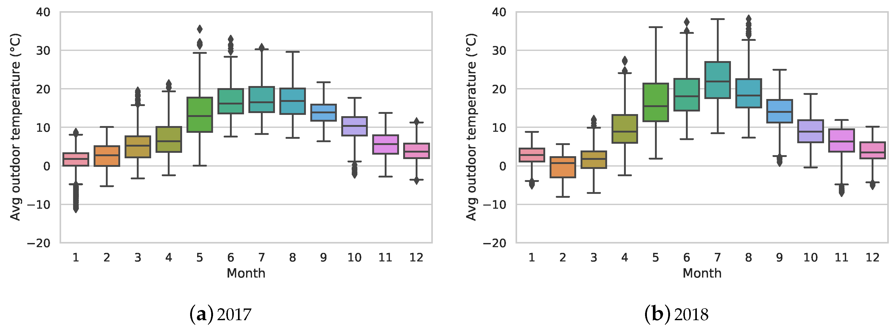
In this study, we only assess the substations’ behaviour while space heating is needed. Figure 1 shows the yearly seasonality of the outdoor temperature recorded for one building in two consecutive years. As one can see in Figure 1, the average outdoor temperature in 2017 during January–April and November–December is below 10 °C. The heating season in 2018 mainly includes January–April and October–December.

6.2. Data Preprocessing

Missing values can occur for different reasons, such as connection problems with measuring instruments; e.g., energy meters. As we are interested in identifying deviating operational behaviours on a weekly basis, daily time series with more than 25% of missing values (or six missing hours within a 24-h period) are discarded. There are different imputation methods, such as mean substitution, hot-deck imputation [37], regression analysis and multiple imputation [38]. We apply a k-nearest neighbours (kNN)-based approach [39] to impute the missing values; that is, for each feature and year, the missing hours are imputed using the values of the five nearest neighbours (days) and the same hours (we let the number of neighbours, k, be five, which is a default value for the used library). The method identifies the nearest neighbours with the help of Euclidean distances, and the missing values for each hour are weighted by the distance to each neighbour.

Faults in measurement tools can appear as extreme values or sudden jumps in the measured data. We use a Hampel filter [40], which is a median absolute deviation (MAD)-based estimation method, to detect and smooth out such extreme values. The filter computes the median, MAD and the standard deviation (SD) over the data in a local window. We apply the filter with default parameters; i.e., the size of the window is considered to be seven which yields 3-neighbours on each side of a sample and the threshold for extreme value detection is set to be three. Therefore, in each window, a sample with a distance of three times the SD from its local median is considered as an extreme value and is replaced by the local median.

Time series data may contain seasonality—a repeating pattern within a fixed time period. The process of identifying and removing a time series’ seasonal effects is called seasonal adjustment. Seasonal effects can mask other interesting characteristics of the data. Seasonal adjustment helps to better reveal any interesting components and allows better data analysis. In our case study, the data exhibit yearly seasonality. We apply differencing to adjust the seasonality; that is, each observation is subtracted by the value from previous year. We consider three years of data (2016, 2017 and 2018), and this gives us two years of data after seasonality adjustment (the first year of data is skipped to adjust the seasonality). Additionally, since 2016 is a leap year, 29 February is excluded while differencing.

As mentioned above, the proposed approach partitions the available data across the time axis on a weekly basis in order to extract patterns within each week. Therefore, it is necessary to convert the continuous features to categorized or nominal features; i.e., data discretization must be conducted. We apply SAX to transform the time series into a symbolic representation. In order to perform a meaningful comparison between time series with different offsets and amplitudes, the time series need to be normalized; i.e., they need to have a mean of zero and standard deviation of one. Therefore, each yearly time series (feature vector) is normalized with z-score normalization. This step is performed automatically while applying SAX. We consider five categories (alphabet size) for the SAX transformation process as follows: low, low_medium, medium, medium_high and high. Nevertheless, the alphabet size can be adjusted based on the available data. In the previous study [10], we considered four categories; i.e., the same as the number of season periods. However, due to the risk of losing information, the fifth category of medium is added.

6.3. Data Segmentation and Pattern Extraction

The size of the time window (partition) for pattern extraction is important for further analysis. A proper partition length allows us to monitor the operational behaviour of the substations rather than the residents’ behaviour. Therefore, after performing some preliminary tests and having discussions with domain experts, the time window was set to be a week. The PrefixSpan algorithm is used to identify frequent sequential patterns with a desired length. Any patterns that satisfy the user-specified threshold are considered as frequent. For the studied problem, the user-specified threshold is set to be one; i.e., any patterns that appear at least once will be considered. In addition, due to the importance of the selected features, the desired length of pattern is set to be equal to the number of features, which is five.

6.4. Affinity Propagation Parameter Tuning

AP has a number of parameters. In this study, we adjust two of these parameters, namely affinity and damping. The affinity parameter is set to be pre-computed since the algorithm is fed with a similarity matrix. The damping factor can be regarded as a slowly converging learning rate to avoid numerical oscillations. It is within a range of 0.5 to 1.0. We always apply AP with a damping factor equal to 0.5; in the case that convergence does not occur, the damping factor will be increased by 0.05 units and AP will be rerun with a new damping factor until convergence occurs.

6.5. Implementation and Availability

The proposed approach is implemented in Python version 3.6. The Python implementations of the PrefixSpan algorithm and the edit distance are fetched from [41,42], respectively. The AP algorithm and SAX are adopted from the scikit-learn module [43] and the pyts: A python package for time series classification [44], respectively. To construct and manipulate an MST, the NetworkX package is used [45]. The package uses Kruskal’s algorithm to construct the MST. The implemented code and the experimental results are accessible via GitHub through the following link: https://github.com/shahrooz-abghari/HOM-Real-World-Datasets.

7. Results and Discussion

We have studied the operational behaviour of the substations of 47 buildings during a period of two years (2017 and 2018). For each building, we first modelled the substation’s weekly operational behaviour; this was performed by grouping the extracted frequent patterns into clusters of similar patterns. In order to monitor the substations’ performance, we analysed and assessed the similarity between substation’s behaviours for every two consecutive weeks. When the bi-weekly comparison showed more than 25% (a user-specified threshold) difference and if the average temperature was less than or equal to 10 °C, further analysis was conducted by integrating the produced clustering solutions into a consensus clustering. The obtained consensus clustering solution was used to build an MST, where the exemplars were tree nodes and the distances between them represented the tree edges. In order to identify unusual behaviours, the longest edge of the MST was removed. The smallest sub-trees created by the cut were interpreted as faults or deviations.

7.1. Substations Bi-Weekly Performance Signature

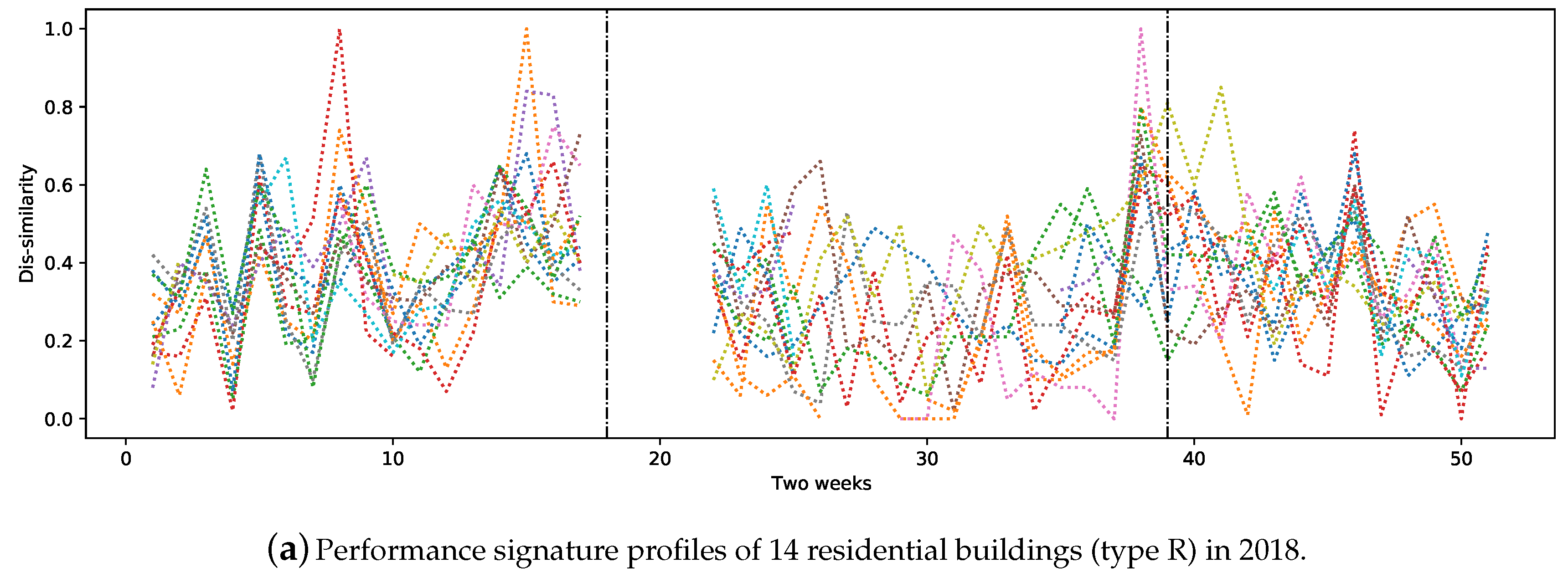
As mentioned above in Section 4.3, the assessed similarities of a substation’s operational behaviour can be used to build the substation performance signature profile for the entire studied period. Additionally, such profiles can be used to compare substations belonging to the same heat load category. We studied four types of buildings: C, R, R-C, and S (see Table 2 for more information). Figure 2a shows the signature profiles of 14 residential buildings in 2018. The area between the two vertical dashed lines represents the non-heating season in all figures. Figure 2b depicts the performance signature profiles of the substations of nine company buildings for the same year. Figure 2c contains the largest number of buildings belonging to the R-C category; i.e., 20 in total. Figure 2d represents the signature profiles of four schools. All the studied buildings are located in the same city. As one can see, Figure 2a–d contains signatures that are quite similar in the period of week 1 until week 18 (1 January–6 May 2018) and week 45 to week 46 (5–18 November 2018).

Although the expectation was to observe similar performance signatures from buildings in the same category, some substations showed quite different behaviours. The main reasons for this can be related to the difference between the average outdoor temperature within two weeks in different areas of the city. Our further analysis showed that buildings of the same type and that are close together tend to have similar performance signature profiles during heating seasons. In addition, the social behaviour of people, special holidays and/or faulty substations and equipment have a high impact on substations’ performance. It is also the case that buildings of same category behave differently, mostly due to installation issues, unsuitable configurations or different brands of equipment. Nevertheless, this requires further analysis by domain experts.

7.2. Modelling Substations’ Operational Behaviour

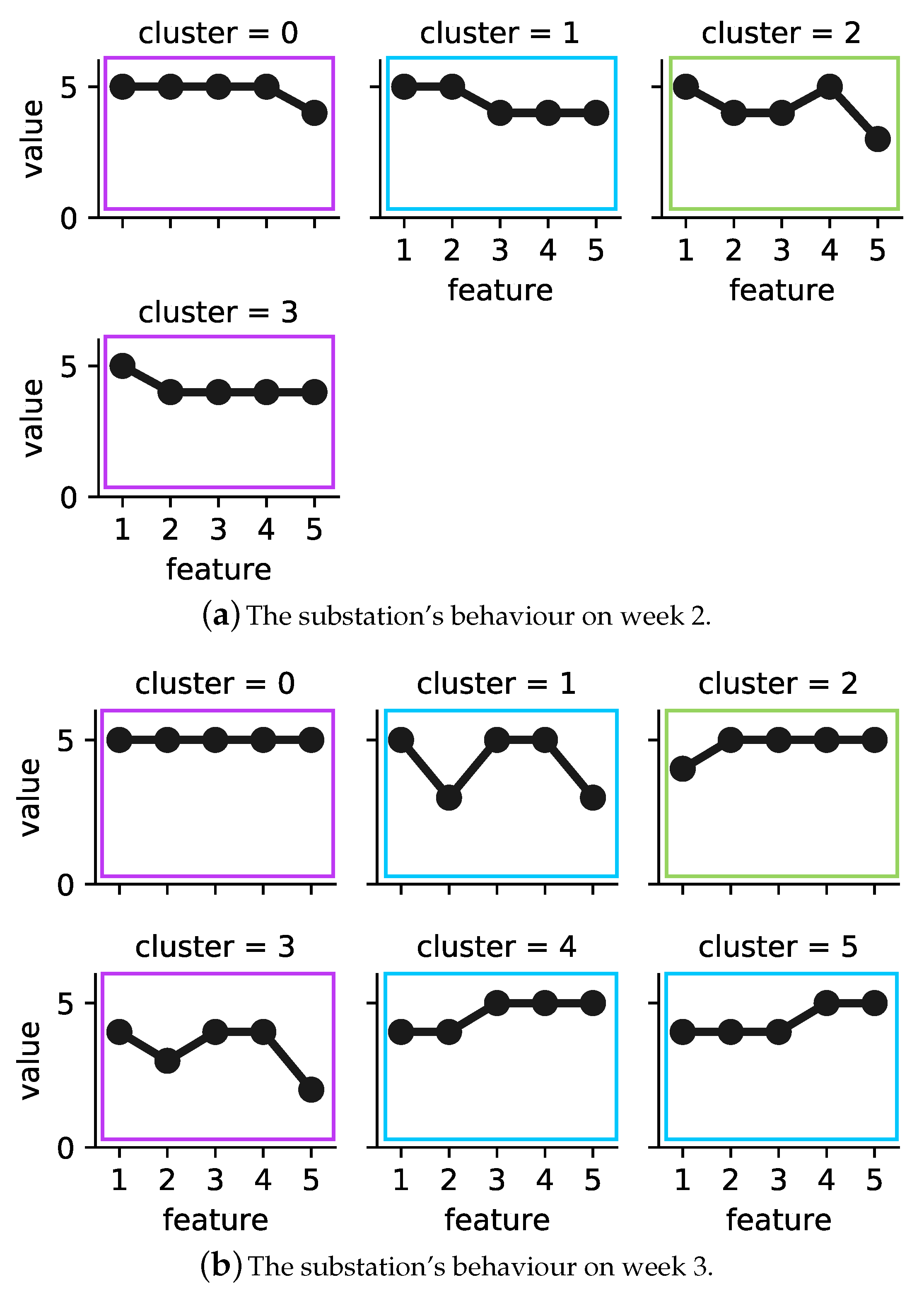
The weekly operational behaviour of a substation can be modelled by clustering the extracted patterns based on their similarities into groups. Using the AP algorithm, each cluster can be recognized by its exemplar—a representative pattern of the whole group. Each cluster models the substation’s operational behaviour for some hours up to a couple of days based on its frequency. The number of clusters in each clustering solution can be interpreted as different operational modes of the substation for the studied week. High number of clusters may due to the same reasons as those discussed in the section above, such as the difference between outdoor temperatures during the days and nights. The extracted patterns contain five features. Each feature can belong to one of five available categories: low, low_medium, medium, medium_high and high.

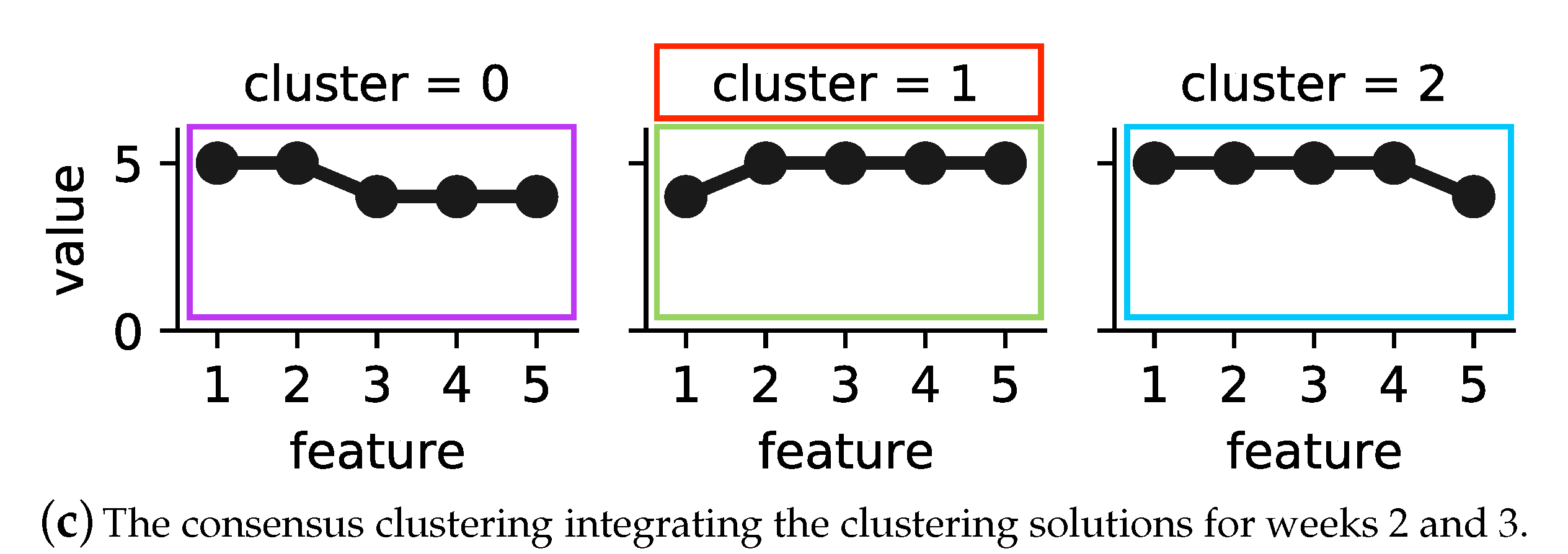
Figure 3 shows the operational behaviour of building B_3’s substation during weeks 2 and 3 in 2017, where low is represented by one and high by five, respectively. Note that each category is the result of differencing to adjust yearly seasonality for each feature. Figure 3a represents four operational behaviour modes of building B_3’s substation during the second week of 2017. Cluster 2 covers 57 h, the largest number of hours among the sample, while cluster 1 covers only 26 h, which is the lowest number of hours. In week 3 (see Figure 3b), six operational behaviour modes were detected. Cluster 3 in this week, similar to cluster 2 in week 2, covers 57 h. Cluster 4, with the lowest number of hours, covers only 11 h.

We further analysed the operational behaviour models of weeks 2 and 3 by calculating the similarity between the exemplars of the corresponding clustering solutions. The calculated dissimilarity was above 25%, and the average weekly outdoor temperature was below 10 °C. Therefore, the proposed method integrated the clustering solutions into consensus clustering. Figure 3c represents the operational behaviour model of the substations for the studied two weeks. The model contained three clusters. In order to detect deviating behaviour, as explained previously in Section 4.3, first an MST was built on top of the consensus clustering solution. Next, the longest edge of the tree was removed, and sub-trees with the smallest size and that were far from majority of data could be marked as deviating behaviour. In Figure 3c, cluster 1 (framed in red) is detected as an outlier.

Table 4. Number of identified daily deviating behaviours in weeks 2 and 3 for building B_3 in 2017.

Weekly Cluster	Consensus Cluster (CC)
	CC0	CC1	CC2
W2,C0			7
W2,C1	6
W2,C2		7
W2,C3			7
W3,C0			6
W3,C1	4
W3,C2		4
W3,C3			6
W3,C4	5
W3,C5	5
Total days	12	11	14

and

Table 5. Identified hourly deviating behaviours in weeks 2 and 3 for building B_3 in 2017.

Weekly Cluster	Consensus Cluster (CC)
	CC0	CC1	CC2
W2,C0			37
W2,C1	26
W2,C2		57
W2,C3			48
W3,C0			26
W3,C1	30
W3,C2		23
W3,C3			57
W3,C4	11
W3,C5	21
Total hours	88	80	168

show the distribution of each weekly cluster together with the number of days and hours that they cover across the consensus clustering solution, respectively. As one can see, in Table 4, the detected operational behaviours in week 2 are divided into four groups, while week 3 contains six categories of different operational behaviours. In week 2, the majority of the behaviours appear across the whole week, except cluster 1, which covers only 6 days. In week 3, on the other hand, clusters 1 and 2 contain operational behaviours observed within 4 days. Clusters 4 and 5 cover 5 days and the last two remaining clusters cover 6 days. Considering the consensus clustering solution, cluster 1 contains the least number of days, at 11, while clusters 0 and 2 include 12 and 14 days, respectively. Note that weekly clustering solutions can have a daily overlap; however, they cover different hours.

Table 5 shows the number of hours covered by each weekly cluster and the total hours for each bi-weekly cluster (consensus cluster). As one can see, consensus cluster 2 contains the most number of hours, at 168. Cluster 0 and 1 cover 88 and 80 h, respectively, within weeks 2 and 3. As mentioned above, by cutting the longest edge of the built MST on top of the consensus clustering solution, the smallest and most distant cluster can be considered as deviating behaviour; i.e., consensus cluster 1. This cluster appears in 11 days (Table 3, consensus cluster CC1) and in total 80 times (Table 4, consensus cluster CC1) out of 336 (24 h × 14 days). The data collected for these particular days could be further analysed by domain experts to obtain a better insight and understanding of the identified deviating behaviour.

In general, an increase or decrease in the number of observed clusters in one week in comparison to its neighbouring week can be interpreted as an indication of deviating behaviours. This can occur for different reasons such as a sudden drop in outdoor temperature. Therefore, in order not to take into account every single change as deviating behaviour, we considered the use of a performance measure called overflow. The measure expresses a substation’s performance in terms of the volume flow per unit of energy flow. In the DH domain, the overflow of a well-performing substation is expected to be 20 $\frac{l}{kWh}$. Therefore, by computing a substation’s weekly overflow, any bi-weekly detected deviations in conjunction with weekly overflow above 20 could be flagged as real changes in the substation.

Table 6. Substations with bi-weekly deviating behaviours on an hourly basis and an overflow of more than 20 in 2017 and 2018.

Year	Substation	C	R	R-C	S
2017	B_L	2
	B_3			88
	E_D_32_A		14
	G_3		6
	M_S		14
	O_S				6
	P_S				1
	R_4	4
	S_1		61
	S_10	40
	S_2A_C	1
	S				1
	V_S				3
	Total	47	95	88	11
Year	Substation	C	R	R-C	S
2018	B_3			64
	C_T	2
	E_D_32_A		2
	F_12_18	21
	M_S		46
	R_4	1
	S_		38
	S_10	9
	S_2D-F	5
	V_S				1
	Total	38	86	64	1

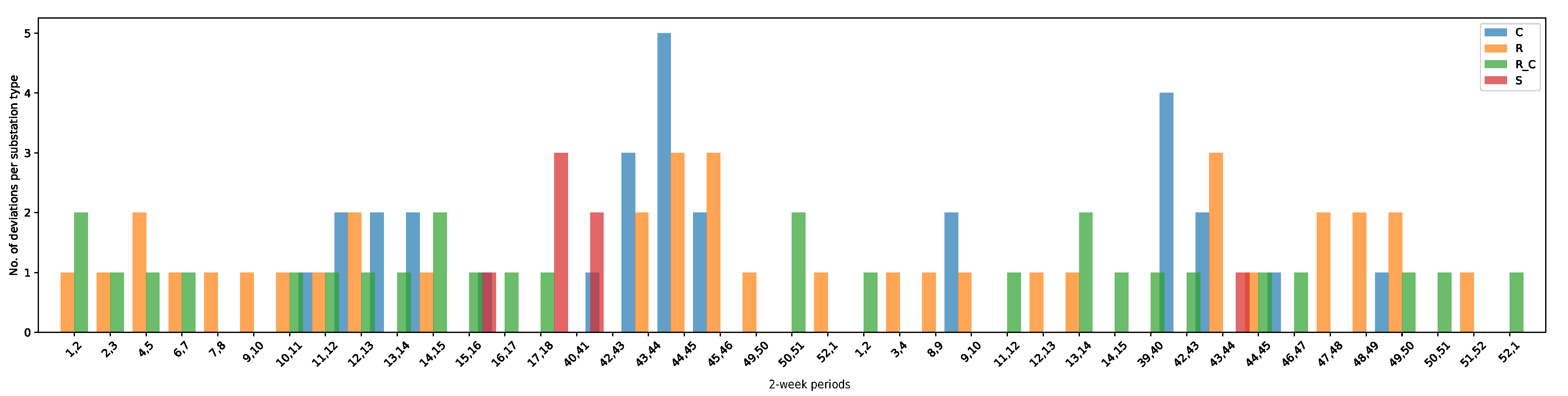
Note. Substations in bold are those that had deviating behaviours in both 2017 and 2018. C: company, R: residential, R-C: residential and company, S: school.

represents substations with bi-weekly deviating behaviours on an hourly basis and an overflow of more than 20 in 2017 and 2018. In general, substations that belong to the residential category had the highest number of deviating behaviours in both years; i.e., four substations had 95 and three substations had a total of 86 detected deviating behaviours in 2017 and 2018, respectively. In the residential–company category, there was only one substation which in both years contained a considerable number of deviating behaviours; i.e., 88 and 64. The company category contained four substations with 47 and five substations with 38 exhibited deviating behaviours in 2017 and 2018, respectively. For the school category, all four substations contained in total 11 detected deviating behaviours in 2017, while in 2018, only one of these substations contained one deviating behaviour. In Table 6, those substations that appear in both years are shown in bold.

Figure 4 summarizes the statistics of Table 6 on a daily basis for the four categories in 2017 and 2018. The plot can help domain experts in identifying categories with the largest number of daily deviating behaviours for a specific time period. For example, substations belonging to company and residential categories had the largest number of deviating behaviours during weeks 42 to 45 in 2017.

7.3. Patterns Representative of Deviating Behaviours

Extracted patterns can provide meaningful information for domain experts; i.e., each pattern represents the status of the five selected features at a specific time period. Note that each category shows the status of a feature at time t in comparison to its value in time $365-t$. As mentioned in Section 6.2, the yearly seasonality of the data is adjusted by the differencing method.

Table 7. Top 10 weekly patterns detected as outliers in 2017 and 2018 in total.

No.	Pattern	Count
1	high,high,high,high,high	80
2	high,high,high,high,medium_high	63
3	medium_high,medium,medium_high,medium_high,medium	39
4	medium,medium,medium,medium,medium_high	39
5	low,high,low_medium,low_medium,high	21
6	medium,medium_high,medium,medium,high	15
7	medium_high,low_medium,medium,medium_high,low_medium	13
8	medium_high,medium_high,medium,medium,medium	13
9	low_medium,low_medium,medium,medium,medium	11
10	medium,medium,low,low,medium	7

shows the top 10 weekly patterns detected as deviating behaviours in 2017 and 2018. These patterns are exemplars (representative) of the bi-weekly consensus clustering solutions. As one can see in all patterns except pattern number 7, features 3 and 4 (shown in bold in the table)—the primary heat and primary mass flow rate, respectively—hold similar values.

Table 8. Top weekly patterns detected as outliers with respect to building types in 2017 and 2018.

Year	No.	Type	Pattern	Count
2017	1	R-C	high,high,high,high,medium_high	57
	2	R	high,high,high,high,high	55
	3	C	medium_high,low_medium,medium,medium_high,low_medium	13
	4	R	low_medium,low_medium,medium,medium,medium	11
	5	C	medium_high,medium_high,medium,medium,medium	10
	6	R-C	medium,medium,medium,medium,medium_high	8
	7	C	medium,medium,low,low,medium	7
	8	S	medium,medium,medium,medium,medium_high	6
	9	R-C	medium,high,low_medium,low_medium,high	5
	10	R-C	medium,low_medium,low_medium,low_medium,low_medium	5
2018	1	R-C	medium_high,medium,medium_high,medium_high,medium	39
	2	R	medium,medium,medium,medium,medium_high	25
	3	R	high,high,high,high,high	24
	4	C	low,high,low_medium,low_medium,high	21
	5	R	medium,medium_high,medium,medium,high	15
	6	R-C	high,high,high,high,medium_high	6
	7	R	high,medium,high,high,medium	5
	8	C	low,low,medium_high,high,low_medium	5
	9	C	high,low_medium,medium,medium_high,low_medium	4
	10	R-C	medium_high,high,high,medium,high	4
	11	R-C	medium_high,medium_high,medium_high,medium_high,high	4

Note. Patterns in bold occurred in both years.

shows the top weekly patterns based on the four categories of buildings. The majority of patterns only occurred for specific types of substations, except the pattern “medium, medium, medium, medium, medium_high”, which was observed for the types R-C and S in 2017 (row 6 and 8) and R in 2018 (row 2). Patterns belonging to residential–company and residential categories were the most frequent in number overall. In addition, some of these patterns re-occurred in both 2017 and 2018 for the same categories of substations, as shown in bold in the table.

7.4. Substation Performance

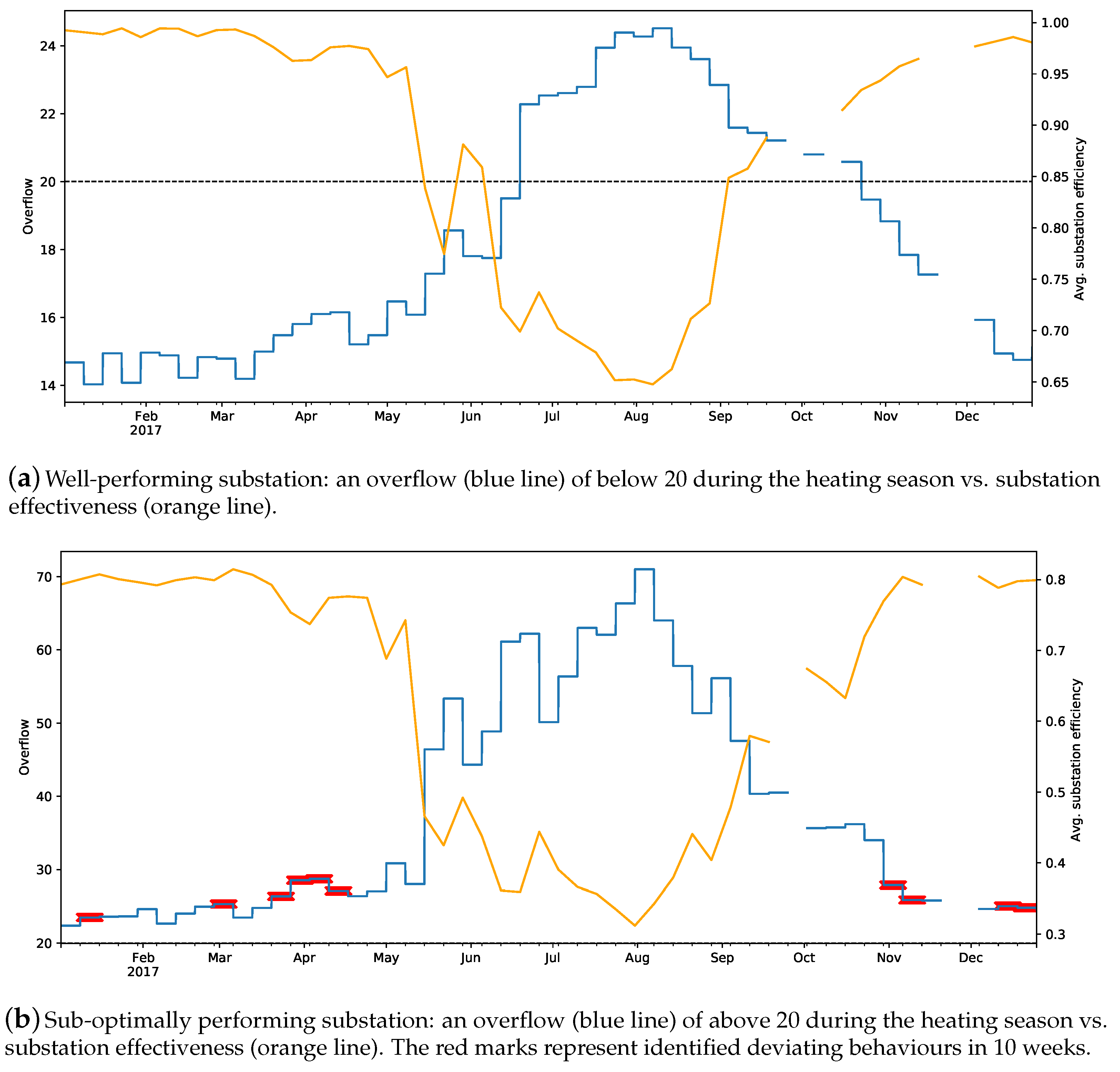
The substation efficiency, $E_s^T$, can be used as an indicator to assess a substation’s operational behaviour throughout the entire year. Figure 5 depicts the detected deviations for two substations belonging to the residential category, using their average efficiency and overflow for year 2017. Figure 5a, represents a well-performing substation. Notice that the substation’s efficiency on average is around 98%. In addition, the weekly substation’s overflows for the whole heating season (January–May and November–December) are below 20. Figure 5b, on the other hand, shows a substation with sub-optimal performance during 2017. As one can see, the substation’s efficiency on average is around 80% during the heating season. Moreover, the weekly overflows for the whole year are above 20. In addition, the proposed approach identified deviating behaviours in 10 weeks, which are marked with red.

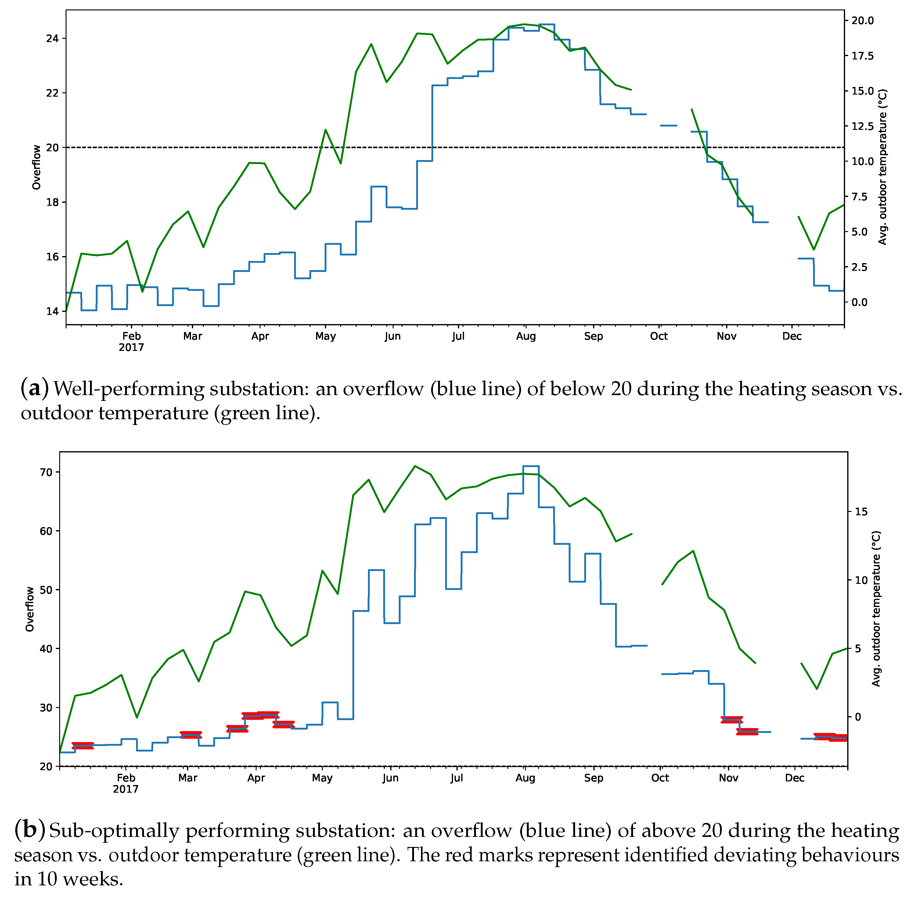
Figure 6 represents the performance of the same substations based on their weekly overflow and outdoor temperature. It is noticeable in Figure 6b that whenever the outdoor temperature exhibits a sudden change, the proposed approach observes that as deviating behaviour.

Notice that in this study we only consider the smallest sub-trees after cutting the longest edge of an MST as outliers. Nevertheless, one can consider sorting the sub-trees based on their size from smallest to the largest for further analysis. Alternatively, by defining a domain-specific threshold, any edges with a distance greater than the threshold can be removed, and further analysis can be performed on smaller sub-trees.

8. Conclusions and Future Work

We have proposed a higher order data mining approach to analyse real-world datasets. The proposed approach combines different data analysis techniques to (1) build a behavioural model of the studied phenomenon, (2) use the built model to monitor the phenomenon’s behaviour, and (3) finally to identify and further analyse deviating behavioural patterns. At each step, adequate information is supplied which can facilitate the domain experts in their decision making and inspection.

The approach has been demonstrated and evaluated on a case study from the district heating (DH) domain. For this purpose, we have used data collected for a three-year period of 47 operational substations belonging to four different heat load categories. The results have shown that the method is able to identify and analyse deviating and sub-optimal behaviours of the DH substations. In addition, the proposed approach provides different techniques for monitoring and data analysis, which can allow domain experts to better understand and interpret the DH substations’ operational behaviour and performance.

In future work, we aim to pursue the further analysis and evaluation of the proposed approach on similar scenarios in different application domains; e.g., the approach can be applied to monitor and analyse the behavior and performance of fleets of wind turbines. In addition, we want to extend the proposed approach with means for root-cause analysis and the diagnosis of detected deviations.

References

- Isermann, R. Fault-Diagnosis Systems: An Introduction from Fault Detection to Fault Tolerance; Springer: Berlin/Heidelberg, Germany, 2006. [Google Scholar]
- Hodge, V.; Austin, J. A survey of outlier detection methodologies. Artif. Intell. Rev. 2004, 22, 85–126. [Google Scholar] [CrossRef] [Green Version]
- Chandola, V.; Banerjee, A.; Kumar, V. Anomaly detection: A survey. ACM Comput. Surv. 2009, 41, 15. [Google Scholar] [CrossRef]
- Zhang, Y.; Meratnia, N.; Havinga, P. Outlier detection techniques for wireless sensor networks: A survey. IEEE Commun. Surv. Tutor. 2010, 12, 159–170. [Google Scholar] [CrossRef] [Green Version]
- Gupta, M.; Gao, J.; Aggarwal, C.C.; Han, J. Outlier detection for temporal data: A survey. IEEE Trans. Knowl. Data Eng. 2014, 26, 2250–2267. [Google Scholar] [CrossRef]
- Aggarwal, C.C. Outlier Analysis; Springer International Publishing: Cham, Switzerland, 2017. [Google Scholar]
- Isermann, R. Supervision, fault-detection and fault-diagnosis methods—An introduction. Control Eng. Pract. 1997, 5, 639–652. [Google Scholar] [CrossRef]
- Katipamula, S.; Brambley, M.R. Methods for fault detection, diagnostics, and prognostics for building systems—A review, part I. Hvac R Res. 2005, 11, 3–25. [Google Scholar] [CrossRef]
- Katipamula, S.; Brambley, M.R. Methods for fault detection, diagnostics, and prognostics for building systems—A review, part II. Hvac R Res. 2005, 11, 169–187. [Google Scholar] [CrossRef]
- Abghari, S.; Boeva, V.; Brage, J.; Johansson, C.; Grahn, H.; Lavesson, N. Higher order mining for monitoring district heating substations. In Proceedings of the 2019 IEEE International Conference on Data Science and Advanced Analytics (DSAA), Washington, DC, USA, 5–8 October 2019; pp. 382–391. [Google Scholar]
- Fontes, C.H.; Pereira, O. Pattern recognition in multivariate time series—A case study applied to fault detection in a gas turbine. Eng. Appl. Artif. Intell. 2016, 49, 10–18. [Google Scholar] [CrossRef]
- Sánchez-Fernández, A.; Baldán, F.; Sainz-Palmero, G.; Benítez, J.; Fuente, M. Fault detection based on time series modeling and multivariate statistical process control. Chemom. Intell. Lab. Syst. 2018, 182, 57–69. [Google Scholar] [CrossRef]
- Djenouri, D.; Laidi, R.; Djenouri, Y.; Balasingham, I. Machine Learning for Smart Building Applications: Review and Taxonomy. ACM Comput. Surv. 2019, 52, 24. [Google Scholar] [CrossRef]
- Gadd, H.; Werner, S. Fault detection in district heating substations. Appl. Energy 2015, 157, 51–59. [Google Scholar] [CrossRef] [Green Version]
- Xue, P.; Zhou, Z.; Fang, X.; Chen, X.; Liu, L.; Liu, Y.; Liu, J. Fault detection and operation optimization in district heating substations based on data mining techniques. Appl. Energy 2017, 205, 926–940. [Google Scholar] [CrossRef]
- Capozzoli, A.; Lauro, F.; Khan, I. Fault detection analysis using data mining techniques for a cluster of smart office buildings. Expert Syst. Appl. 2015, 42, 4324–4338. [Google Scholar] [CrossRef]
- Månsson, S.; Kallioniemi, P.O.J.; Sernhed, K.; Thern, M. A machine learning approach to fault detection in district heating substations. Energy Procedia 2018, 149, 226–235. [Google Scholar] [CrossRef]
- Calikus, E.; Nowaczyk, S.; Sant’Anna, A.; Gadd, H.; Werner, S. A Data-Driven Approach for Discovery of Heat Load Patterns in District Heating. arXiv 2019, arXiv:1901.04863. [Google Scholar]
- Paparrizos, J.; Gravano, L. k-shape: Efficient and accurate clustering of time series. In Proceedings of the 2015 ACM SIGMOD International Conference on Management of Data, Melbourne, Victoria, Australia, 31 May–4 June 2015; pp. 1855–1870. [Google Scholar]
- Sandin, F.; Gustafsson, J.; Delsing, J. Fault Detection with Hourly District Energy Data: Probabilistic Methods and Heuristics for Automated Detection and Ranking of Anomalies; Svensk Fjärrvärme: Stockholm, Sweden, 2013. [Google Scholar]
- Roddick, J.F.; Spiliopoulou, M.; Lister, D.; Ceglar, A. Higher order mining. ACM Sigkdd Explor. Newsl. 2008, 10, 5–17. [Google Scholar] [CrossRef]
- Pei, J.; Han, J.; Mortazavi-Asl, B.; Pinto, H.; Chen, Q.; Dayal, U.; Hsu, M. Prefixspan: Mining sequential patterns efficiently by prefix-projected pattern growth. In Proceedings of the 17th International Conference on Data Engineering, Heidelberg, Germany, 2–6 April 2001; pp. 215–224. [Google Scholar]
- Frey, B.J.; Dueck, D. Clustering by passing messages between data points. Science 2007, 315, 972–976. [Google Scholar] [CrossRef] [Green Version]
- MacQueen, J. Some methods for classification and analysis of multivariate observations. In Proceedings of the Fifth Berkeley Symposium on Mathematical Statistics and Probability, Oakland, CA, USA, 1 January 1967; Volume 1, pp. 281–297. [Google Scholar]
- Gionis, A.; Mannila, H.; Tsaparas, P. Clustering Aggregation. ACM Trans. Knowl. Discov. Data 2007, 1, 4-es. [Google Scholar] [CrossRef] [Green Version]
- Boeva, V.; Tsiporkova, E.; Kostadinova, E. Analysis of Multiple DNA Microarray Datasets. In Springer Handbook of Bio-/Neuroinformatics; Springer: Berlin/Heidelberg, Germany, 2014; pp. 223–234. [Google Scholar]
- Goder, A.; Filkov, V. Consensus Clustering Algorithms: Comparison and Refinement. In Proceedings of the 2008 Tenth Workshop on Algorithm Engineering and Experiments (ALENEX), San Francisco, CA, USA, 19 January 2008; pp. 109–234. [Google Scholar]
- Lin, J.; Keogh, E.; Wei, L.; Lonardi, S. Experiencing SAX: A novel symbolic representation of time series. Data Min. Knowl. Discov. 2007, 15, 107–144. [Google Scholar] [CrossRef] [Green Version]
- Levenshtein, V.I. Binary codes capable of correcting deletions, insertions, and reversals. Sov. Phys. Dokl. 1966, 10, 707–710. [Google Scholar]
- Aggarwal, C.C.; Yu, P.S. Outlier detection for high dimensional data. In Proceedings of the 2001 ACM SIGMOD International Conference on Management of Data, Santa Barbara, CA, USA, 21–24 May 2001; Volume 30, pp. 37–46. [Google Scholar]
- Jiang, M.F.; Tseng, S.S.; Su, C.M. Two-phase clustering process for outliers detection. Pattern Recognit. Lett. 2001, 22, 691–700. [Google Scholar] [CrossRef]
- Müller, A.C.; Nowozin, S.; Lampert, C.H. Information theoretic clustering using minimum spanning trees. In Joint DAGM (German Association for Pattern Recognition) and OAGM Symposium; Springer: Berlin/Heidelberg, Germany, 2012; pp. 205–215. [Google Scholar]
- Wang, X.; Wang, X.L.; Wilkes, D.M. A minimum spanning tree-inspired clustering-based outlier detection technique. In Industry Conference on Data Mining; Springer: Berlin/Heidelberg, Germany, 2012; pp. 209–223. [Google Scholar]
- Wang, G.W.; Zhang, C.X.; Zhuang, J. Clustering with Prim’s sequential representation of minimum spanning tree. Appl. Math. Comput. 2014, 247, 521–534. [Google Scholar] [CrossRef]
- Kruskal, J.B. On the shortest spanning subtree of a graph and the traveling salesman problem. Proc. Am. Math. Soc. 1956, 7, 48–50. [Google Scholar] [CrossRef]
- Frederiksen, S.; Werner, S. District Heating and Cooling; Chapter 10; Studentlitteratur: Lund, Sweden, 2013; Volume 579, p. 465. [Google Scholar]
- Ford, B.L. An overview of hot-deck procedures. Incomplete Data Sample Surv. 1983, 2, 185–207. [Google Scholar]
- Rubin, D.B. Multiple imputations in sample surveys—A phenomenological Bayesian approach to nonresponse. In Proceedings of the Survey Research Methods Section of the American Statistical Association; American Statistical Association: Alexandria, VA, USA, 1978; Volume 1, pp. 20–34. [Google Scholar]
- Troyanskaya, O.; Cantor, M.; Sherlock, G.; Brown, P.; Hastie, T.; Tibshirani, R.; Botstein, D.; Altman, R.B. Missing value estimation methods for DNA microarrays. Bioinformatics 2001, 17, 520–525. [Google Scholar] [CrossRef] [Green Version]
- Hampel, F.R. A general qualitative definition of robustness. Ann. Math. Stat. 1971, 42, 1887–1896. [Google Scholar] [CrossRef]
- Gao, C. PrefixSpan: Python Implementation Source Code. Available online: https://github.com/chuanconggao/PrefixSpan-py (accessed on 2 November 2020).
- Jain, B. Edit Distance: Python Implementation Source Code. Available online: https://www.geeksforgeeks.org/dynamic-programming-set-5-edit-distance (accessed on 2 November 2020).
- Pedregosa, F.; Varoquaux, G.; Gramfort, A.; Michel, V.; Thirion, B.; Grisel, O.; Blondel, M.; Prettenhofer, P.; Weiss, R.; Dubourg, V.; et al. Scikit-learn: Machine Learning in Python. J. Mach. Learn. Res. 2011, 12, 2825–2830. [Google Scholar]
- Faouzi, J.; Janati, H. pyts: A Python Package for Time Series Classification. J. Mach. Learn. Res. 2020, 21, 1–6. [Google Scholar]
- Hagberg, A.; Swart, P.; Chult, D.S. Exploring Network Structure, Dynamics, and Function Using NetworkX; Technical Report; Los Alamos National Lab. (LANL): Los Alamos, NM, USA, 2008. [Google Scholar]
Figure 1.
Yearly seasonality of the outdoor temperature for one specific building.
Figure 2.
Performance signature profiles of substations based on building types. Due to missing values, some of the bi-weekly comparisons are missing. The area between two vertical dashed lines in each plot represents the non-heating season. In all of the above plots, each color represents a performance signature profile of a substation.
Figure 3.
Building B_3’s substation’s operational behaviour in weeks 2 and 3 in 2017. Each cluster is shown by its exemplar. The colored frames represent the consensus clustering solution, where purple = cluster 0, green = cluster 1 and blue = cluster 2. The exemplars of clusters 0 and 2 are chosen from week 2, and cluster 1 is chosen from week 3. After building an MST on top of the consensus clustering solution, cluster 1 is identified as the deviating behaviour of the substation due to its small size and distance from the majority of the data.
Figure 4.
Number of substations with bi-weekly deviating behaviours on a daily basis and their categories during the heating season in 2017 and 2018.
Figure 5.
Example of well and sub-optimally performing substations in 2017. Overflow vs. substation efficiency. Due to missing values, some of the weeks are missing.
Figure 6.
Example of well and sub-optimally performing substations in 2017. Overflow vs. outdoor temperature. Due to missing values, some of the weeks are missing.