Development of a Reduced Order Model of Solar Heat Gains Prediction

Abstract

The aim of this study was to elaborate and validate a reduced order model able to forecast solar heat gains as a function of the architectural parameters that determine the solar heat gains. The study focused on office buildings in Catalonia and Spain and their physical values were taken from the Spanish Building Technical Code and European Union Directive 2018/844. A reduced order model with three direct variables (solar heat gain coefficient, shade factor, window to wall ratio) and one indirect design variable (building orientation) was obtained and validated in respect to the International Performance Measurement and Verification Protocol. Building envelope properties were fixed and the values were taken from the national standards of Spain. This work validates solar heat gain coefficient as a primary variable in determining the annual solar heat gains in a building. Further work of developed model could result in building energy need quick evaluation tool in terms of solar heat gains for architects in building early stage as it has an advantage over detailed building simulation programs in terms of instant calculation and the limited need for predefined input data.

1. Introduction

Solar energy is the largest untapped energy source, which used in a smart way can result in great active and passive energy savings in building sector. There are different ways to take advantage of the free energy source of solar energy and methods vary between the concept of passive and active solutions and by the investment cost. Even though solar energy is used as a passive solution that can compensate the heating demand of a building, the thermal performance of a building should be analyzed on an annual basis, as excessive solar heat gains in the summer period can result in overheating and an increase of cooling demand [1]. In terms of new buildings, passive solar solutions should be considered in the early design stages of the building, as with simple measures it is possible to reduce the high amount of CO₂ emissions in building sector, as it is the largest source of emissions in European Union [2]. The typical and time-consuming way of analyzing internal gains from solar radiation is using a dynamic simulation software, which requires the knowledge of an expert. Therefore, for making solar calculations accessible for a regular user, there is a need to develop simplified energy calculators that require reduced order models.

In this work, a reduced order model or solar heat gains was suggested and validated. There were 4 key design variables (window to wall ratio (WWR), solar heat gain coefficient (SHGC), shade factor and orientation of the building) chosen for creating the model, that were considered to hold the main importance when defining the behavior of solar heat gains. While creating the reduced order model, it was noted, that SHGC has the capacity to define the solar heat gains with acceptable precision, while not taking convective heat transfer into consideration. SHGC, often referred to as g-value or solar coefficient, is the sum of the solar direct transmittance and the secondary heat transfer factor towards the inside. The second component consists of heat transfer by convection and longwave infrared radiation of that part of the incident solar radiation, that has been absorbed by the glazing [3]. The value of SHGC has to be measured when the fenestration system is under recommended standard conditions of ISO 19467, which requires the internal temperature of +20 °C and external of 0 °C. The required internal surface coefficient of heat transfer is 8 W/m²·K and external 24 W/m²·K. Net radiation flux of incident radiation for the case of normal incidence is 300 W/m². The tolerance for the air temperature or environmental temperature difference between sides during the measurements shall be ±5 °C [4].

In previous studies, these design parameters, such as window-to-wall ratio, building orientation, and glazing materials, have been studied separately from the influence of solar heat gains. It has been well established that the orientation of the building has an impact on the energy consumption of the building, as well as the area of the glazed surfaces, as the entering solar radiation contributes to a heating demand through the energy absorbed in the interior furnishings and the internal partition. Therefore, the glazing properties, mainly expressed by solar heat gain coefficient, and shading of the windows, are holding the important place in reduction of the entering solar heat gains [5,6,7,8]. In this study an overall conclusion was brought to a concept of a reduced order model. The current work focused on the solar radiation that is transmitted through the windows of a building, contributing to the energy balance by absorbing the transmitted energy in surfaces inside and reradiating the long-wave thermal radiation, which in the end is defined as solar heat gains. The transient simulation software Energy Plus, that was used for simulations, calculates solar heat gains with the Perez solar model [9]. The purpose of the proposed reduced order model was to propose a simplified version of the Energy Plus evaluation of solar heat gains. Some models pay special attention to the solar radiation absorbed and reflected by the interior [10,11], but in Energy Plus, the detailed simulation software, taken as a reference, does not simulate that phenomena when computing the solar heat gains. Hence, the reduced model will be developed without taking into account that phenomena. Nevertheless, leaving that phenomena out can result in an error from 3 to 8% according to [12].

In the first part of the work, a parametric study was carried out with Energy Plus and the correlation between solar heat gains and chosen building design parameters was obtained. In the second part of the study a reduced order model based on the physical phenomena was developed and validated in accordance with the International Performance Measurement and Verification Protocol [13].

2. Methods

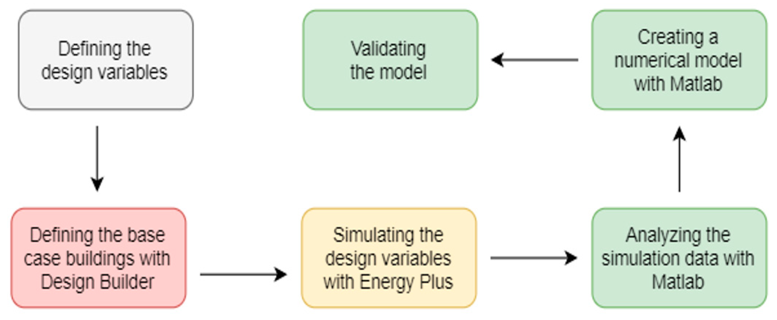
The work was divided into six phases, as expressed in Figure 1. In order to create the most adequate model possible, key design variables of a building had to be chosen. As there was no previous work carried out by the author to define the key variables, the decision was based on previous research carried out in building thermal analysis sector [14,15,16]. Before launching the simulations, design variable ranges and simulation base cases had to be defined. Therefore 4 base buildings were chosen, with a detailed data from building engineering guide book of Spain [17]. The design phase of current work was carried out with Design Builder [18], where the building shape was drawn, given the construction values, and defined the activity and mechanical systems inside. The building base cases were simulated in 12 climate zones of Spain with transient energy simulation software EnergyPlus [19]. Data analyses were done in Matlab [20].

2.1. Identification of the Design Variables

For developing a fast prediction model for determining the effect of the main influencing parameters on solar heat gains, four variables (SHGC, WWR, shade factor, and orientation) were chosen. Physical and simply determinable variables were chosen in order to be beneficial for the architects for direct use in a building design stage. Design variables were chosen based on previous research done in the building energy performance sector, pointing out the key aspects that influence solar heat gains in a building.

2.2. First Design Variable: Shade Factor

Shading devices, whether vertical or horizontal ones, are directly affecting the sunlight entering the room and therefore participating in a decrease or increase in thermal energy loads of the building [14]. Detailed understanding of shading factor is of great importance for determining the solar heat gains in a building. Even though window to wall ratio is the main influencer of the energy loads of the building [16], proper evaluation of shading can make a great difference [21]. The impact of shading is often underestimated in the building design phase, even though detailed analyze of shading systems can result in significant energy savings, especially in summer months in compensation of cooling loads [15]. Shading factor is described as a ratio between the irradiance presence of shading obstacles and irradiance in absence of obstacles. Shading factor value can be represented as follows:

$$F_{\mathrm{s}}=\frac{I_{\mathrm{ţ},\mathrm{s}}}{I_{\mathrm{t}}}$$

(1)

where F_s is the shading factor,

$I_{\mathrm{ţ},\mathrm{s}}$ is global irradiance on a shaded surface, W/m²

I_t is global irradiance, that should reach the surface in absence of shading, W/m²

To provide a specific understanding of shading factor, the previous equation can be expressed explicitly as follows [15]:

$$F_S= \frac{F_{s,b} ·I_b + F_{s,d}·I_d + I_r}{I_b + I_d + I_r}$$

(2)

where $F_{s,b}$ is the geometric shading coefficient for direct radiation

$F_{s,d}$ is the geometric shading coefficient for diffuse radiation

$I_b$ is the direct irradiance in absence of shading obstacles, W/m²

$I_d$ is the diffuse irradiance in absence of shading obstacles, W/m²

$I_r$ is the reflected irradiance in absence of shading obstacles, W/m²

By simplified meaning, the shade factor is the ratio of shaded area of the window, being 0, when there is no shading and 1, when the window is fully shaded. This understanding allows the architects to use shade factor as direct and fast input data, being caused whether by shading objects of a window or nearby buildings, trees, or other influencing aspects. For fast evaluation of the shade factor, for Mediterranean region, values could be obtained from the Spanish Base Document of Energy Savings [17], which, depending on the geometry of different shade, suggests numerical averaged values for fast energy demand prediction.

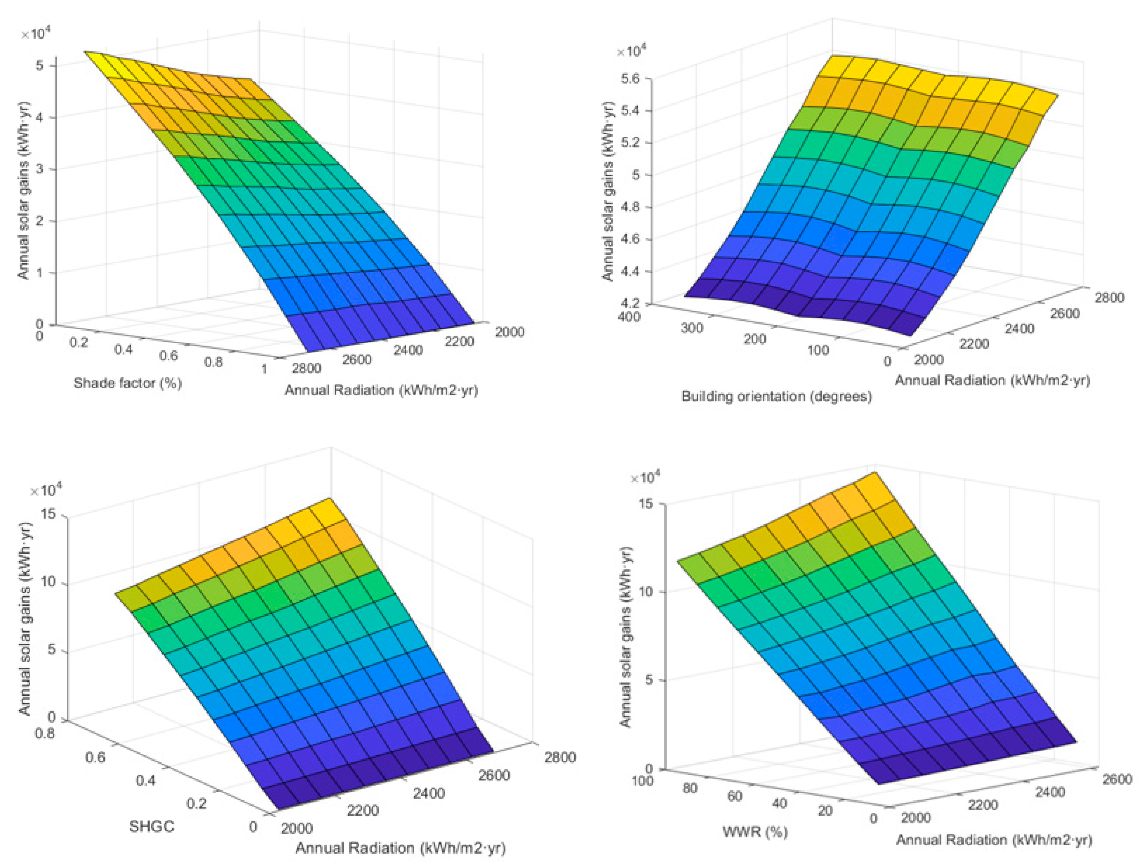
The equations above show, that the relationship between shade factor and reduced radiation rate $I_{\mathrm{ţ},\mathrm{s}}$ is proportional, which gives the leads to the conclusion that also the relationship between solar heat gains and shade factor should be linear.

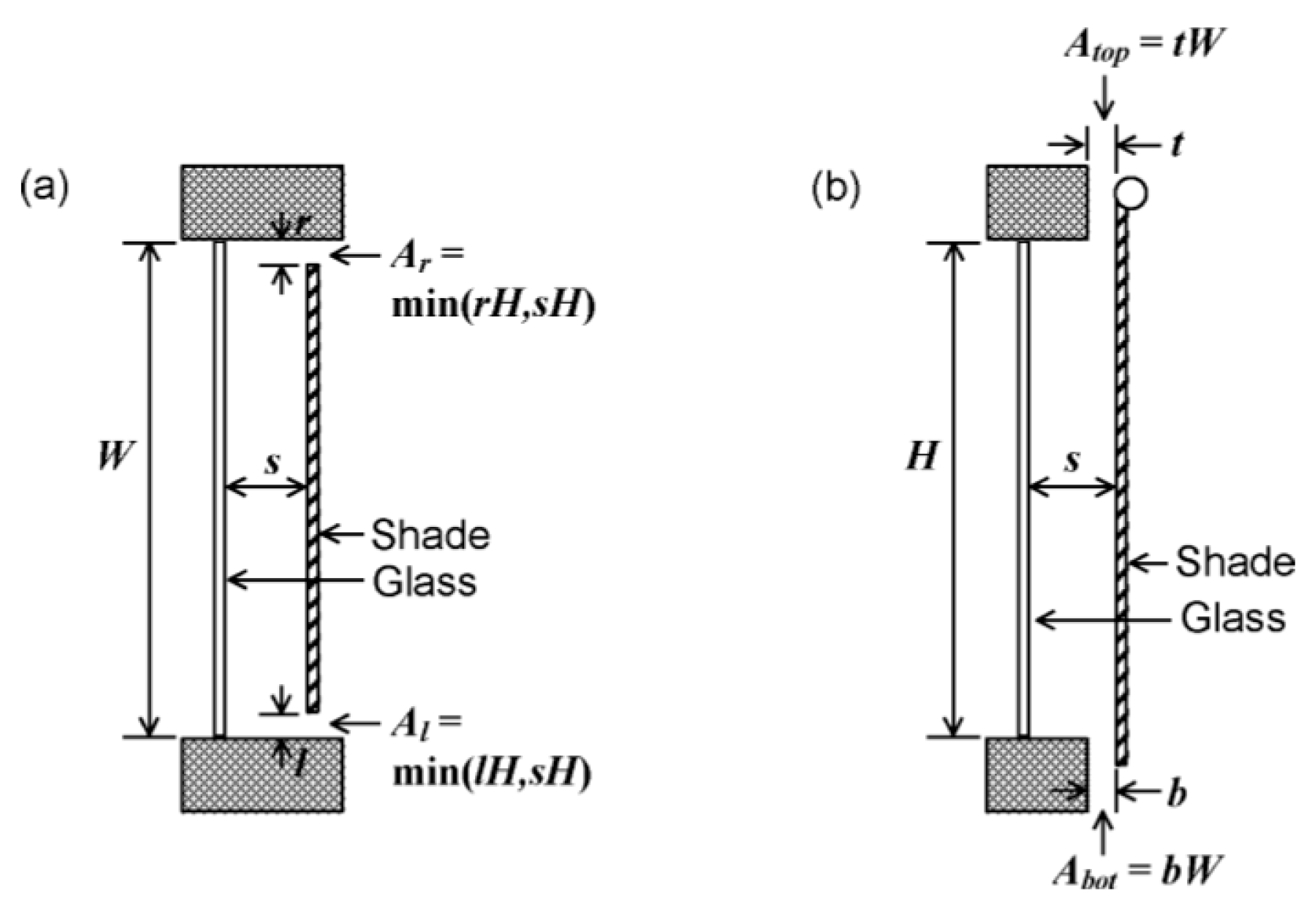
Shade factor represents the shaded area ratio of the window, varying from 0 to 1. Shade factor does not carry information about specific shading device type, as it represents only the percentage of shaded area of a window. Energy Plus simulations were carried out to obtain desired shade factor ratio, while adding shade to the windows and using the theoretical approach of varying the transparency of the shade. EnergyPlus considers shade as a parallel layer to the window, as shown in Figure 2, independent of angle of incidence. When used, shade is assumed to cover all the glazed area, dividers included [22].

2.3. Second Design Variable: Window to Wall Ratio (WWR)

For aesthetics and for daylighting purposes, glazed building facades are often used in modern office buildings. Solar radiation that is transmitted through the glass heats up the surfaces inside the zone that after some time become heat sources [14]. Therefore, as largescale fenestration can bring great benefits in daylighting, thermal effect should be considered with respect. Solar heat gains in a building has a high dependence on transparent surfaces. Even though the opaque surfaces contribute to the energy demand of a building, transparent areas have a more significant influence [16]. For describing how big a part of the wall is occupied by the window, the ratio of window and wall (WWR) is often used and is expressed as follows:

$$\mathrm{WWR}=\frac{{{\displaystyle \sum }}^{ }Glazing area, {\mathrm{m}}^2}{{{\displaystyle \sum }}^{ }Gross exterior wall area, {\mathrm{m}}^2}$$

(3)

WWR = 0 refers to a wall without the window, and WWR = 100 to a wall, which has total glass façade. A visual expression of this can be seen in Figure 3 below.

The formula of window to wall ratio reveals that window area is whether reduced or increased proportionally with the WWR, therefore also the possible solar radiation that can hit the transparent surface is influenced proportionally. This means that the expected relationship between solar radiation and therefore the solar heat gains is linear.

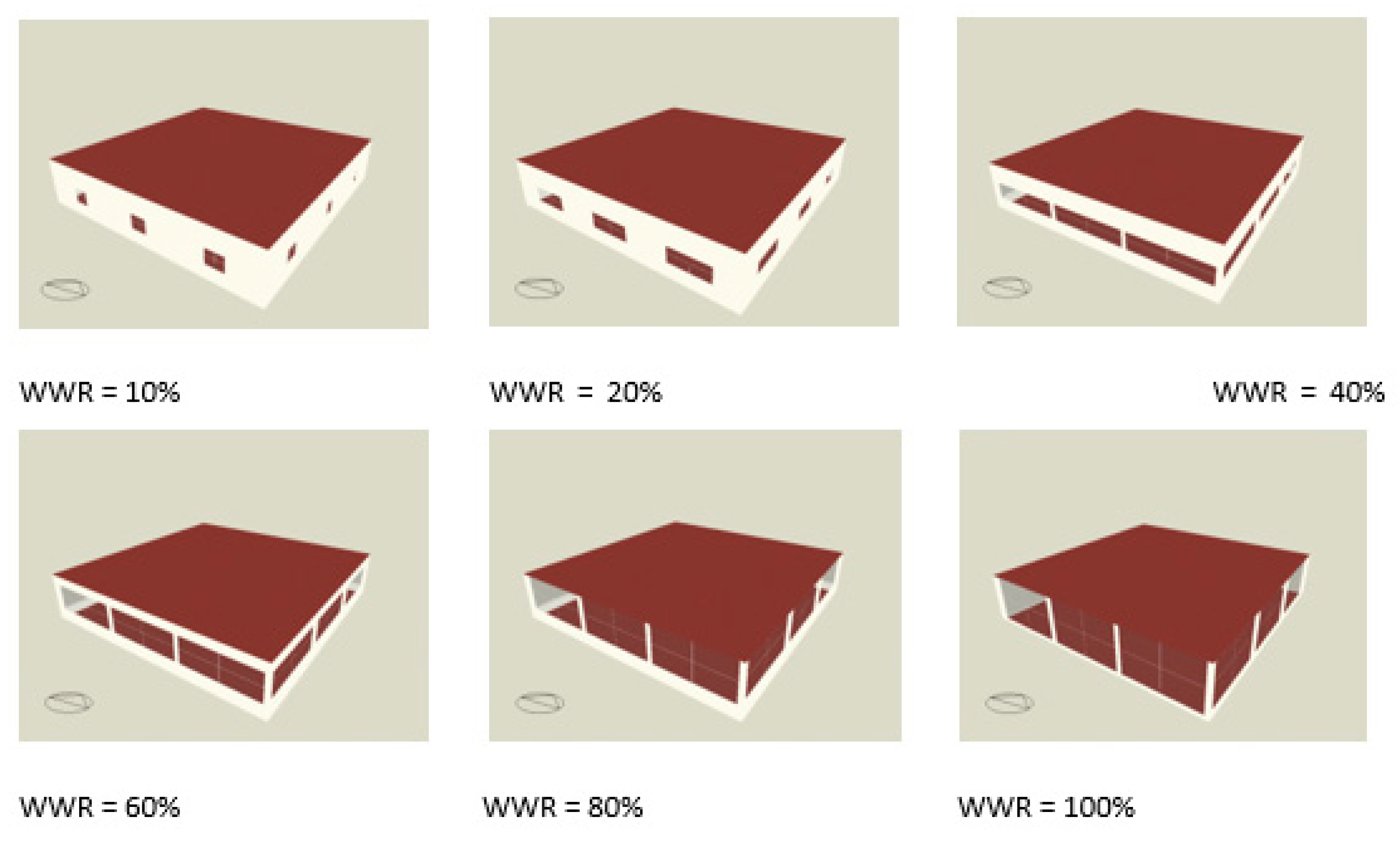
In those simulations WWR was chosen as a design variable, which was given values over WWR = 10…100, which is illustrated in the following graphs (Figure 4):

2.4. Third Design Variable: Building Orientation

Building orientation is considered as an important building design variable, as different facades are sunlit on different hours and intensities of a day, due to the sun path that causes incident radiation angle and direction variations. Therefore, building orientation should be analyzed in a building design stage by the architects. Often the decision of orientation is made by the best accessibility or landscape, even though building orientation affects the amount of solar radiation that enters through the opaque and transparent surfaces. As building orientation has an impact on heating and cooling loads, this important design variable should be considered in the preliminary building design stage [14].

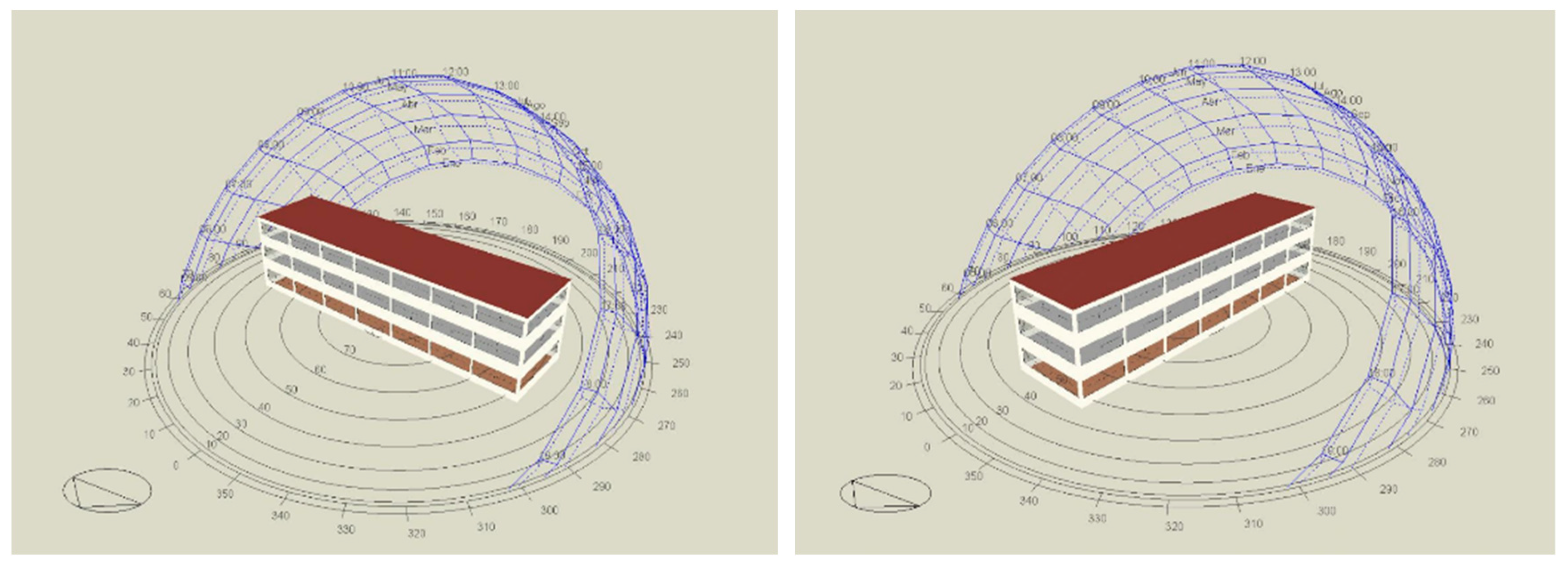
Building base case orientation 0 represents the shorter side of the building facing north, as illustrated in Figure 5. In the following simulations, the building was rotated over 360 degrees.

2.5. Fourth Design Variable: Solar Heat Gain Coefficient

Heat gains from the transparent surfaces of a building have an important part in building’s cooling load, especially in buildings with greater transparent areas [23]. One part of the solar radiation is being transmitted to inner space, a smaller portion of solar radiation gets absorbed in the fenestration, and part of this is transferred to the room as infrared radiation and the other part by convection [24]. $SHGC$ consists of two parts, which are expressed below [25]:

$$SHGC=T_s+A_s·N_i$$

(4)

where $SHGC$ is the solar heat gain coefficient

$T_s$ is the solar transmittance

$A_s$ is the solar absorptance

$N_i$ is the fraction of absorbed solar radiation that enters the room.

Both of the components of SHGC are proportional to solar radiation [26] and therefore also to solar heat gains. This allows to predict the relationship between SHGC and solar heat gains to be linear.

Fourth building design variable was chosen to be SHGC and in order to obtain it, window solar transmissivity was varied from 0 to 0.8.

2.6. Reduced Order Model (ROM)

The main purpose of this study was to elaborate and validate a reduced order model of solar heat gains, to be applicable in monthly method energy calculation. The idea of creating reduced order model relies on simplifying and optimizing the calculations in time and complexity. When determining the key aspects in a complex dynamic system, the model could be created with only the predominant variables. The idea of this approach, called the model order reduction, has the goal to reduce the original degrees of freedom to very small number, while keeping the input-output data accuracy the same [27].

2.7. Simulation

The purpose of the simulations was to observe the numerical data and correlate solar heat gains behavior to the chosen building design variables, to compare the outcome of the simulations with the set hypothesis. Current work was carried out with energy simulation program EnergyPlus, which was fed by the input data created with Design Builder. Energy Plus is a free software developed by the Department of Energy (DOE, USA) which is validated for energy simulation. The software contains tools in order to run a large number of simulations, as well as parametric simulations.

In order to obtain general overview of building thermal performance in Spain, simulations were carried out in all twelve climate zones of Spain. Spanish climate zones are categorized by the summer and winter severity rates. Climate zone A3 represents the climate with the mildest summer and winter, while zone E1 with the roughest ones [17].

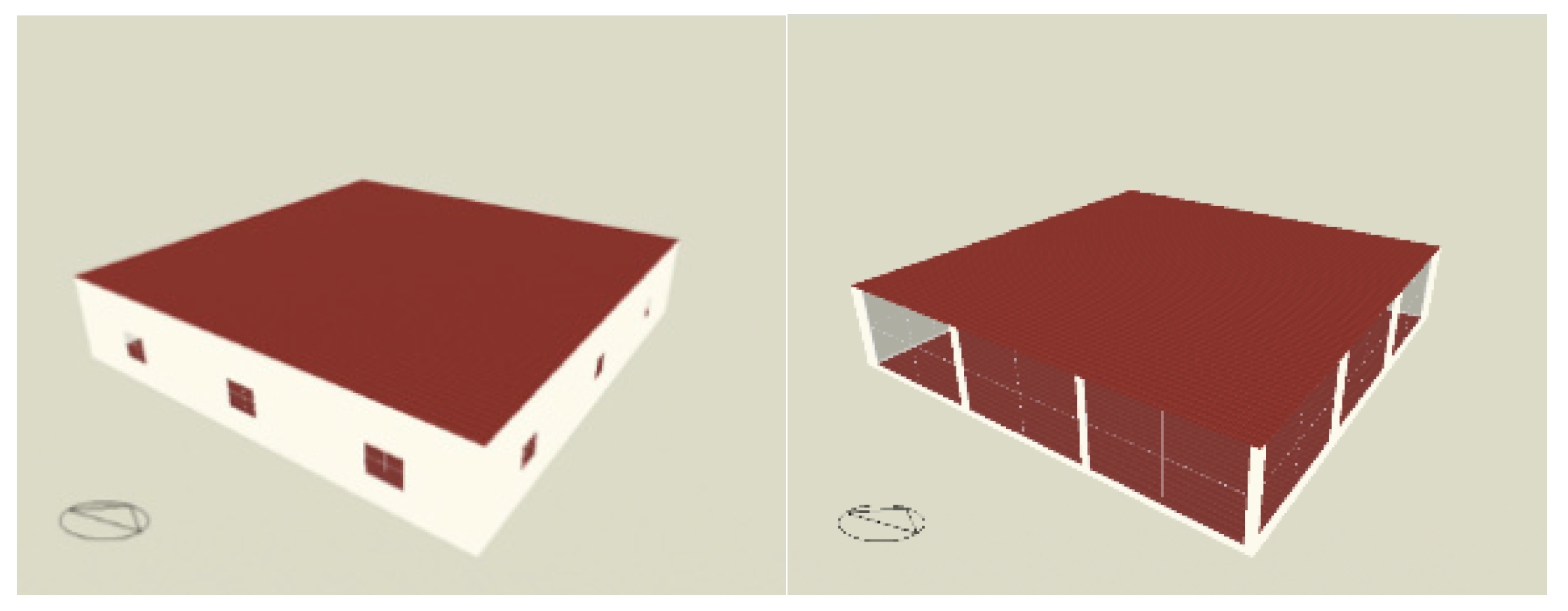
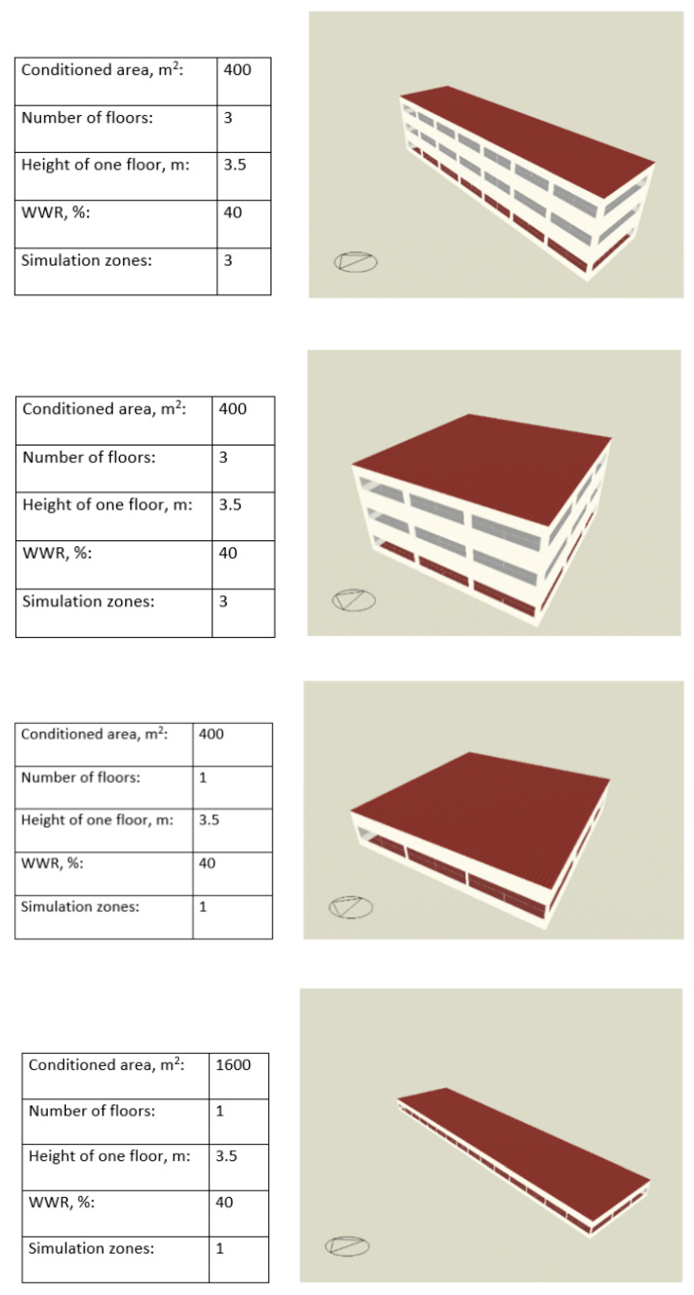
Simulations were carried out with four reference buildings with different floor shapes and number of floors, to ensure the approach was independent from building shape. Each building shape was simulated with respect to the chosen variables.

2.8. Description of Simulation Cases

The base window to wall ratio was chosen to be typical for the office buildings, being 40%. Floor height was chosen 3.5 m in all the cases. Every floor consisted of 1 zone. All the buildings had the shortest side facing the north. The four simulation base cases are presented in Figure 6.

2.9. Solar Radiation Simulations

The analysis of the four design variables were carried out and predicted hypothesis of the behavior were compared to the simulated result in order to determine if the results could be implemented to the numerical model.

Four design variables, namely shade factor, window to wall ratio, orientation, and SHGC, were studied to be applicable for the reduced order model for quick estimation of solar heat gains in a building. As all the design variables proved their importance though their linear relation (Figure 7) to solar heat gains, all four variables were implemented to the developed numerical model. Shade factor, SHGC, and window to wall ratio were added as direct multiplicators of solar radiation and orientation indirectly being attached to every single surface placement through solar angles, as represented in the direct beam radiation calculation.

2.10. Solar Heat Gain Model

As the correlations obtained in the simulation part showed the independence of building shape and climate zones, general conclusions as providing a model, could be done. Chosen design variables, that showed to have linear correlation with solar heat gains, were used as an input data for the designable model, as described in following sections. After the creation of the numerical model, validation was carried out in order to prove the accuracy of the model.

The expectations were to observe linear correlation between simulated solar heat gains and architectural design parameters which in the end were compared to the mathematical calculation of theoretical solar heat gains. The determinable model was expected to show the correlation between theoretical solar heat gains and simulated solar heat gains, which could allow to determine empirical model, with the design variables as an input data.

2.11. Model Development

Numerical model for estimating solar heat gains were obtained through the comparison of simulated results of solar heat gains to the mathematical calculation of solar heat gains. It was expected that similar behavior in both cases would be observed and, in the case of an offset, a correction factor would be provided. Solar radiation could be calculated with known mathematical formulas and the intention was by multiplying the mathematical result with chosen design variables to reach the same values that were simulated. This approach would allow to estimate solar heat gains faster than using an energy simulation program, which requires specialist knowledge for adequate analysis.

The developed model was created while using mathematical expression of solar heat gains, as explained in the next chapter, while integrating chosen simulated building design variables as multipliers of total incident solar radiation.

Following model was suggested:

$$\begin{array}{ll}S{G}_{Building}& = {\displaystyle {\displaystyle \sum }_{i=1}^m}S{G}_{ surface}\\ & ={\displaystyle {\displaystyle \sum }_1^m}{{\displaystyle \int }}^{ }{I}_T\left(t,\theta \right)·WWR·S_{wall}·SHG{C}_{window}·\left(1-S{F}_{window}\right)·dt\end{array}$$

(5)

which, assuming the timestep being 1 h (t = 1), being integrated, takes a form of:

$$\begin{array}{ll}S{G}_{Building}& = {\displaystyle {\displaystyle \sum }_{i=1}^m}S{G}_{ surface}\\ & ={\displaystyle {\displaystyle \sum }_1^m}WWR·S_{wall}·SHG{C}_{window}·\left(1-S{F}_{window}\right)·{{\displaystyle \int }}_1^{n}I\left(t,\theta \right)·dt\\ & ={\displaystyle {\displaystyle \sum }_1^m}WWR·S_{wall}·SHG{C}_{window}·\left(1-S{F}_{window}\right)·t·{\displaystyle {\displaystyle \sum }_1^n}I\left({\theta }_{1\dots n}\right) \end{array}$$

(6)

where $S{G}_{surface}$ is the annual solar heat gains over a surface (kWh),

$I_T$ is total incident radiation on a tilted surface (kWh/m²), found with HDKR model,

n is hours of the year,

m is surfaces of the building,

$S_{wall}$ is the area of a wall (window included, if present) (m²), and

$S_{window}$ is the window area on a surface (m²).

The design variables:

$SHG{C}_{window}$ is the solar heat gain coefficient of the window,

$S{F}_{window}$ is the shade factor of the window, and

$WWR$ is the window to wall ratio.

As is visible from previous equations, 3 out of 4 design variables were directly taken into account—the window to wall ratio, SHGC and shade factor (SF). Now, the indirect information of orientation needs to be taken into account, and this could be done through the solar angles, which means that solar radiation incident and zenith angle need to be calculated.

2.12. The Indirect Calculation of the Third Design Variable: Orientation

The calculation of orientation was obtained through the calculations of incident solar radiation and rotation of the building.

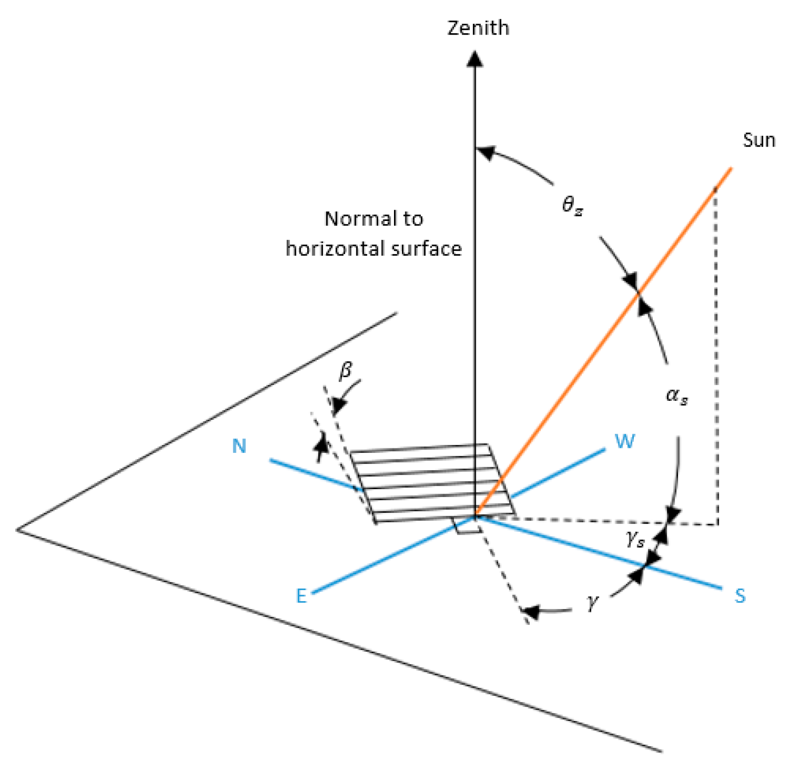
The angle of incidence,$\theta$, is the angle between the solar beam and the normal to the surface. Zenith angle, ${\theta }_z$, is the angle between solar beam and the vertical [28]. Both angles are represented in Figure 8.

In general, orientation information will be taken into account through the beam radiation, as it will be expressed through the cosine ratio of incidence and zenith angle as follows:

$$R_b=\frac{cos\left(\theta \right)}{cos \left({\theta }_z\right)}$$

(7)

Therefore, the cosines of both angles need to be found. As incident and zenith angles are a complex system on many other solar angles, angles of declination, latitude, tilt (or slope of the surface), azimuth, and solar hour need to be calculated. Latitude, tilt, and azimuth will be constants, if we don’t change the location, slope, or orientation of the window, which leaves only declination and solar hour as unknowns. Declination ($\delta$) is the angular location of the sun north of south of the celestial equator, which can vary $-23.45° \le \delta \le 23.45°$, depending only on the day of the year (n), as expressed below [28]:

$$\delta = 23.45·sin \left(\left(284 + n\right)·\frac{360}{365} \right)$$

(8)

For computational methods, there is yet another method available, which requires calculation of two intermediate variables B and E in order to calculate solar time from standard time.

$$B =\left(n-1\right)·\frac{360}{365}$$

(9)

where n is the nth day of the year and B is expressed in radians. E is the equation of time in minutes, expressed as follows:

$$E=229.2·\left(0.000075+0.001868·cos\left(B\right)-0.032077·sin\left(B\right)\right)-0.014615·cos\left(2B\right)-0.04089·sin\left(2B\right))$$

(10)

which results in the final relationship between $Solar time$ and $Standard time$ as follows:

$$Solar time = Standard time + 4 · \left({\lambda }_{st} - {\lambda }_{loc}\right) + E$$

(11)

where ${\lambda }_{st}$ is the standard median of the time zone and ${\lambda }_{loc}$ is the longitude.

Those analysis results in a more precise declination calculation, which was also used for the current work, and is expressed as follows:

$$\begin{gathered} \delta =0.006918-0.399912·cos\left(B\right)+0.070257·sin\left(B\right)-0.006758·cos \left(2B\right) \\ +0.000907·sin \left(2B\right)-0.002697·cos \left(3B\right)+0.00148·sin\left(3B\right) \end{gathered}$$

(12)

For next, the solar hour angle could be calculated, considering hour angle as angular displacement of sun east or west of the local meridian due to the rotation of the Earth on its axis at 15 degrees per hour, on mornings negative, on the afternoons positive, and was found as follows: [28]

$$\mathsf{\omega } = \left(\min - 770\right) · 0.25$$

(13a)

where min is the time in minutes in a given day.

When all the solar angles defined, finally the incident and zenith angle could be calculated and equations are provided below respectively [28]:

$$\begin{gathered} cos \left(\theta \right) = sin \left(\delta \right) · sin \left(\varphi \right) · cos \left(\beta \right) - sin \left(\delta \right) · cos \left(\varphi \right) · sin \left(\beta \right) · cos \left(\gamma \right) \\ + cos \left(\delta \right) · cos \left(\varphi \right) · cos \left(\beta \right) · cos \left(\omega \right) + cos \left(\delta \right) · sin \left(\beta \right) \\ · sin \left(\gamma \right) · sin \left(\omega \right) + cos \left(\delta \right) · sin \left(\varphi \right) · sin \left(\beta \right) · cos \left(\gamma \right) · cos \left(\omega \right) \end{gathered}$$

(13b)

$$cos \left(\theta z\right) = cos \left(\varphi \right) · cos \left(\delta \right) · cos \left(\omega \right) + sin \left(\varphi \right) · sin \left(\delta \right)$$

(14)

Found cosine values are the input data for beam radiation calculation, which will be taken into account in the HDKR incident radiation calculation and therefore will be reflected also in the developed model.

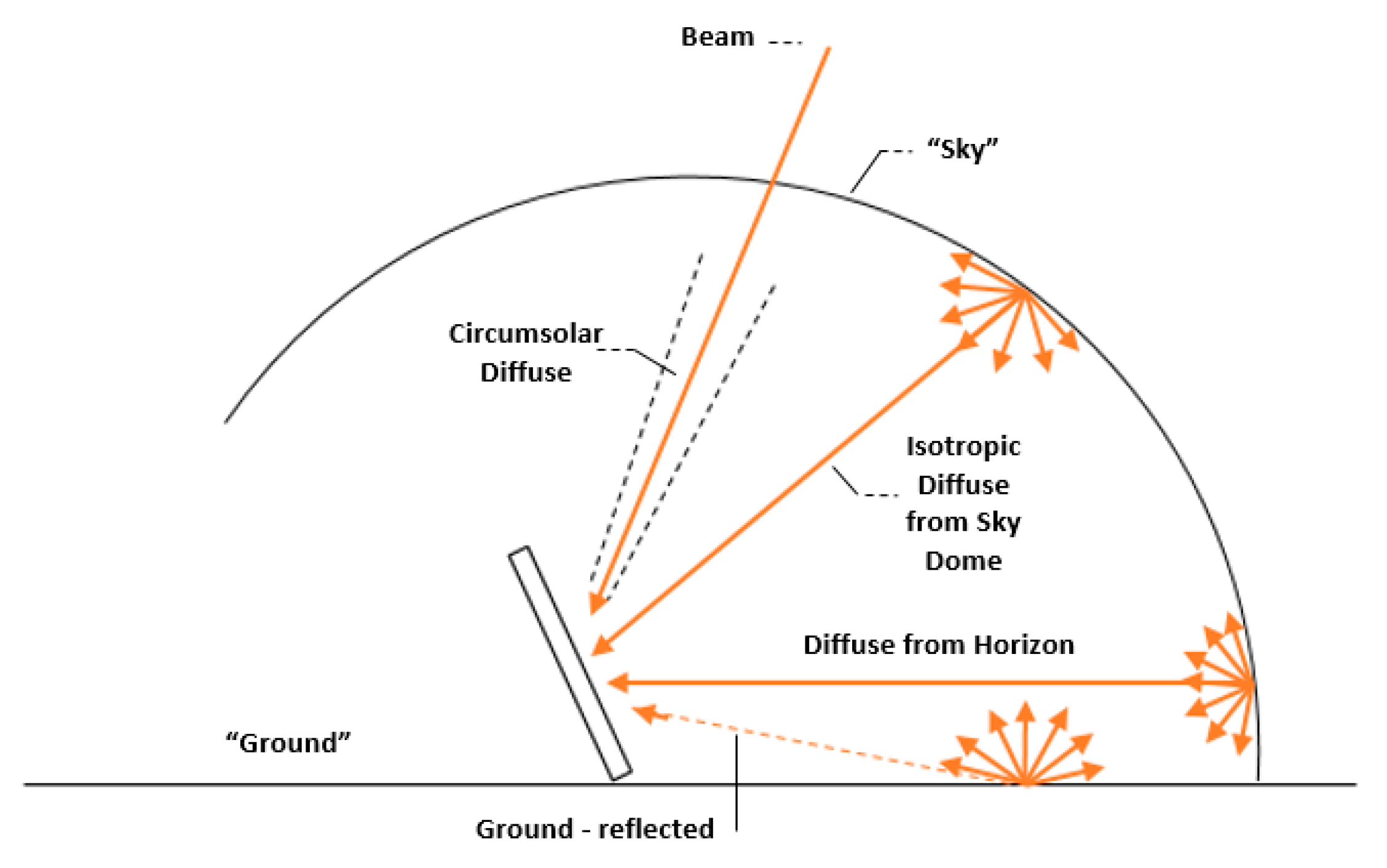
2.13. Calculation of the Total Incident Solar Radiation

In order to calculate solar heat gains, calculation for tilted surfaces had to be found. The incident solar radiation is a combination of beam radiation, diffuse radiation, which has three components, and radiation that has been reflected from the surfaces, that reflect the radiation to the observed surface. Total incident radiation on a tilted surface can be expressed as follows [28]:

$$I_T = I_{T,b} + I_{T,d,iso} + I_{T,d,cs} + I_{T,d,hz} + I_{T,ref}$$

(15)

where $I_{T,b}$ is the total beam radiation, W/m²

$I_{T,d,iso}$ is the total diffuse isotropic radiation, W/m²

$I_{T,d, cs}$ is the total diffuse circumsolar radiation, W/m²

$I_{T,d,hz}$ is the total diffuse horizon radiation, W/m²

$I_{T,ref}$ is the total reflected radiation stream, W/m²

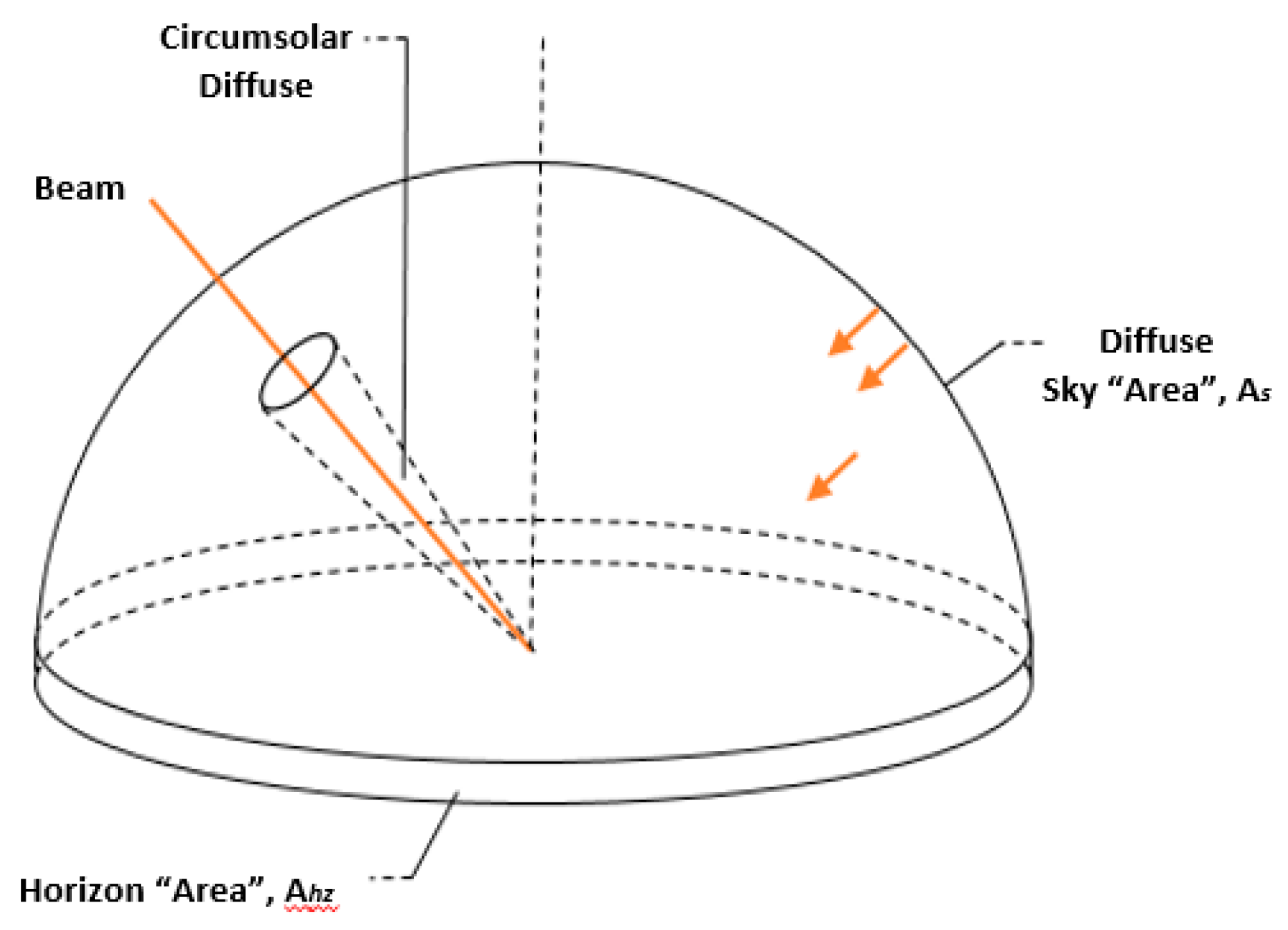
Isotropic radiation is this part of diffuse radiation, that is received uniformly from the entire sky dome. Circumsolar radiation, which is resulting from forward scattering of solar radiation and is being concentrated in the part of the sky around the sun. Horizon brightening radiation is concentrated near the horizon, being the most pronounced in clear skies. Those different radiation parts are expressed in Figure 9 [28].

The total incident radiation that reaches the surface can be expressed as follows:

$$I_T = I_b·R_b+ I_{d,iso}·F_{c-s} + I_{d,cs}·R_b + I_{d,hz}·F_{c-hz} + I_{\rho g} ·F_{c-g}$$

(16)

where $R_b$ is beam radiation,

$F_{c-s}$ is the view factors of circumsolar radiation,

$F_{c-g}$ is the view factors of horizon radiation, and

$I_{\rho g}$ is the remaining reflectance component of radiation being made an assumption, that the reflectance comes only from the ground.

When total incident radiation has been calculated, the ratio between $total radiation on tilted surface$ and $total radiation on horzontal surface$ could be calculated [28].

$$R= \frac{total radiation on tilted surface}{total radiation on horzontal surface}= \frac{I_t}{I}$$

(17)

It is possible to make assumptions that diffuse and ground reflected radiation is isotropic, which means that the sum of diffuse radiation from the sky and reflected radiation from the ground on a tilted surface is the same, no matter the orientation. This way the total radiation on a tilted surface is the sum of beam radiation $I_b·R_b$ and diffuse radiation $I_d$ on horizontal surface and this approach is called isotropic sky model. An improvement on this model is isotropic diffuse model, where radiation is considered to have three components, which are beam radiation, isotropic diffuse radiation and solar radiation that is diffusely reflected from the ground. In this model, total radiation on a tilted surface is a sum of three terms and expressed as follows:

$$I_T = I_{bRb} + I_d \left(\frac{1 + cos\beta }{2}\right) + I_{\rho g}\left(\frac{1 - cos\beta }{2}\right)$$

(18)

where the multipliers of diffuse and reflected irradiance are the view factors to the sky and ground respectively [28]. Even though isotropic diffuse model is easy to use and understand, as there are advanced approaches available, the following method was chosen. There are models that also take into account the circumsolar and horizon lightening radiation in the calculation of solar radiation on a tilted surface [28], as shown in Figure 10:

Hay and Davies (1980) estimated the fraction of diffuse radiation that is circumsolar, considering it all being from the same direction with beam radiation, but they did not take into account the horizon brightening. This aspect was added by Reindl (1990) as was proposed by Klucher (1979), giving the model the name of HDKR. Hay and Davies model is based on an assumption, that all the diffuse radiation can be represented in two parts, namely the isotropic and circumsolar, so the diffuse radiation on tilted surface was written as follows:

$$I_{d,T} = I_{T,d,iso} + I_{T,d,cs}$$

(19)

$$I_{d,T} = I_d·\left(\left(1 - A_i\right)·\left( \frac{1 + cos\beta }{2 }\right)+ A_i·R_b \right)$$

(20)

where A_i is an anisotropy index, which is a function of the transmittance of the atmosphere for the beam radiation, which under clear conditions is high as most of the diffuse radiation will be assumed to be forward scattered. When there is no beam radiation, A_i will be 0 and therefore all the diffuse radiation isotropic and the total radiation on a tilted surface will be expressed as follows:

$$I_T = (I_b + I_d·A_i)·R_b + I_d·\left(1 - A_i\right) ·\left(\frac{1 + cos\beta }{2}\right) + I \rho g ·\left(\frac{1- cos\beta }{2}\right)$$

(21)

Temps and Coulson (1977) added a correction factor to the isotropic diffuse, which was improved by a modulating factor by Klutcher (1979), that would take into account the cloudiness. Reindl (1990) modified the Hay and Davies model with the cloudiness correction factor described earlier, and the final model, that’s also being used in current thesis, is called the HDKR model, as expressed below [28]:

$$I_T = \left(I_b + I_d·A_i\right)·R_b + I_d·\left(1 - A_i\right)·\left(\frac{1 + cos\beta }{2}\right)·\left( 1+\mathrm{f}·{\sin }^3\left(\frac{\beta }{2}\right)\right)+ I_{\rho g} ·\left(\frac{1- cos\beta }{2}\right)$$

(22)

2.14. Validation Case

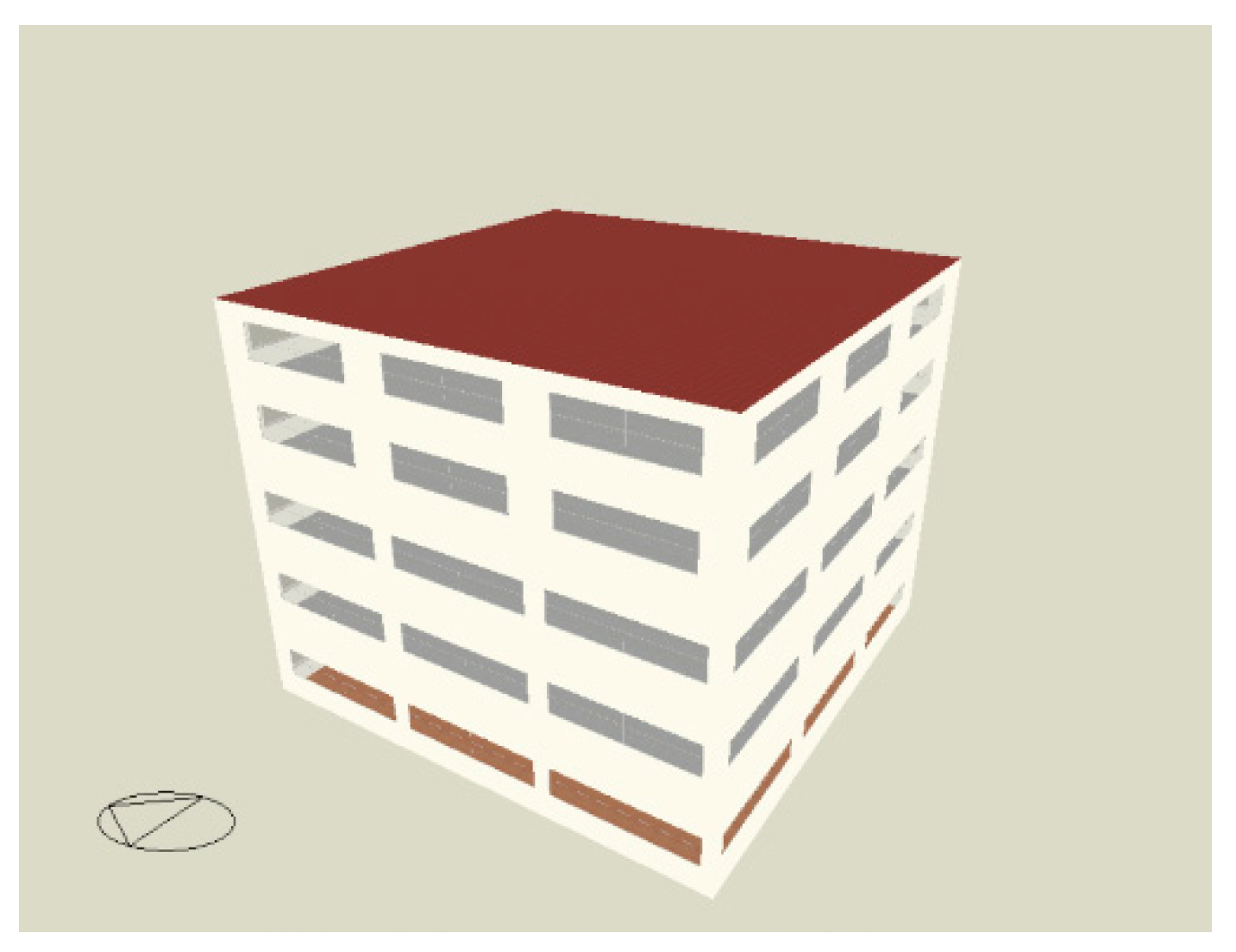
For validating the model, one new building base case was designed with the same constructional parameters as the previous simulations. Annual solar heat gains were simulated with the simulation program EnergyPlus and compared to the value, that was calculated using the developed model. Next, the fifth building shape (Figure 11) was created in Design Builder, and it is expressed below:

The designed building has one floor area of 400 m² and in total 2000 m². Window to wall ratio base case was 40%, as the previous buildings. Chosen validation building was simulated in respect to all the design variables and simulated annual solar heat gains were compared to the calculated solar heat gains, while using the developed model.

2.15. Goodness of Fit of the Model

For calculating the accuracy of the developed model, the coefficient of determination, R² was studied, which is the relation between explained variation in the dependent variable Y to the total variation in Y and can be expressed as follows:

$$R^2=\frac{{{\displaystyle \sum }}^{ } ({\widehat{Y}}_i-\overline{Y}) }{{{\displaystyle \sum }}^{ } (Y_i-\overline{Y}) }$$

(23)

which in the current work is expressed as follows:

$$R^2=\frac{{{\displaystyle \sum }}^{ }{\left(S{G}_{cal{c}_i}-\overline{S{G}_{sim}}\right)}^2 }{{{\displaystyle \sum }}^{ }{\left(S{G}_{si{m}_i}-\overline{S{G}_{sim}}\right)}^2 }$$

(24)

where $S{G}_{cal{c}_i}$ is the value of annual value of solar heat gains, found with new model,

$\overline{S{G}_{sim}}$ is the mean value of all the simulations simulated solar heat gains, kWh

$S{G}_{si{m}_i}$ is the value of annual simulated solar heat gains, kWh

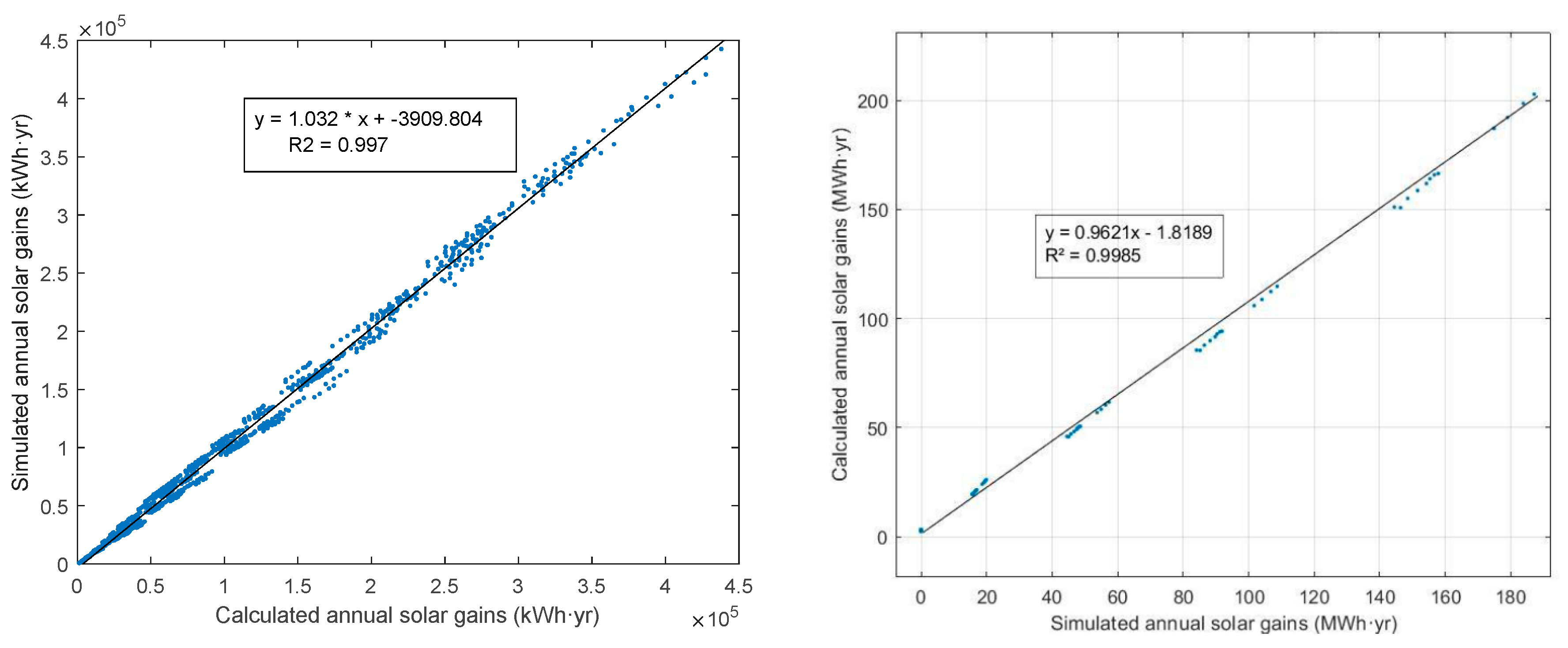
Validation calculation was carried out over all the simulated simulations, and a value of 0.998 was obtained, which is above the suggestion limit [13] as expressed in

Table 1. Calibration limits for IPMVP ¹.

Data Type	Index	IPMVP
Calibration criteria
Hourly criteria %	CV(RMSE)	20
	R2	>0.75

¹ D. Energy and W. Savings, “International Performance Measurement & Verification Protocol,” Renew. Energy, 2002, doi: DOE/GO-102002-1554.

.

The coefficient of determination test should yet only be used for initial check, and therefore standard error of estimate value has to be calculated by International Performance Measurement and Verification Protocol (IPMVP), and the expression is shown below:

$$S{E}_{\widehat{y}}= \sqrt{\frac{{{\displaystyle \sum }}^{ }{\left(\widehat{Y_i}-Y_i\right)}^2}{n-p-1}}$$

(25)

$$S{E}_{\widehat{y}}=\sqrt{\frac{{{\displaystyle \sum }}^{ }{\left(S{G}_{cal{c}_i}-S{G}_{si{m}_i}\right)}^2}{n-p-1}}$$

(26)

where ${\widehat{Y}}_i$ is the calculated value of annual solar heat gains, kWh

$Y_i$ is a simulated annual solar heat gains value, kWh

n is sample size and p is number of independent variables in the regression equation

This expression of statistic is often called as root mean squared error, $RMSE$. To produce the coefficient of variation in root mean squared error, the value of $RMSE$ has to be divided by the mean value of simulated annual solar heat gains, as is expressed below [13]:

$$CV\left(RMSE\right)= \frac{S{E}_{\widehat{y}}}{\overline{Y}}·100\%$$

(27)

$$CV\left(RMSE\right)= \frac{S{E}_{\widehat{y}}}{\overline{S{G}_{sim}}}·100\%$$

(28)

In the case of 4 base case simulation buildings, $CV\left(RMSE\right)$ value, using Equations (26) and (28) was found as follows:

$$CV\left(RMSE\right)= \frac{S{E}_{\widehat{y}}}{\overline{Y}}= \frac{\sqrt{\frac{{{\displaystyle \sum }}^{ }{\left(S{G}_{cal{c}_i}-S{G}_{si{m}_i}\right)}^2}{n-p-1}}}{\overline{S{G}_{sim}}}·100\%$$

(29)

The calculated coefficient of variation in root mean squared error was 6.35% for the training building data and 4.08% for the validation building data, which is lower than allowed 20%, which allows to qualify the quality of the found reduced order model satisfying [29]. To validate the linearity of the correlation between calculated and simulated annual solar heat gains, the previously found statistical correlation with the R² of 0.997 and 0.999, respectively, as calculated by Equation (24) is represented in Figure 12.

3. Conclusions

A reduced order model, able to forecast solar heat gains as a function of the architectural parameters that determine the solar heat gains, was provided and validated. The study was carried out in the Mediterranean climate, based on the energy efficiency regulations of Spain [17].

In order to create a reduced order model for predicting solar heat gains, the key variables that determine the amount of solar heat gains were detected and shade factor, SHGC, window to wall ratio, and building orientation were chosen. Predicted behavior between solar heat gains and chosen design variables were observed and analyzed and found to be applicable for the model. The predicted behavior of the chosen design variables was expected to be proportional to the solar radiation, which allowed us to assume the relation between solar heat gains and the chosen design variables. Shade factor, SHGC, and WWR were implemented in the model as direct multipliers of incident solar radiation. The building orientation was taken into consideration indirectly through the calculation of total radiation through the incident and zenith angle.

The simulated solar heat gains were compared to the calculated solar heat gains, which were obtained by using the developed reduced order model, which involved the mathematical calculation of total irradiance as an implementation. The results obtained demonstrated a high statistical correlation with a square root value of 0.9985.

The reduced order model of solar heat gains was developed and validated in respect to the International Performance Measurement and Verification Protocol (IPMVP) [13] having the coefficient of variation in root mean squared error of 4.08%, which was below the allowed 20%, which allowed to qualify the quality of the found reduced order model. This developed model will allow architects in a building predesign stage to benefit from the option to make fast assumptions of solar heat gains in a building when varying the chosen design variables. Further work in this area could involve the implementation of this reduced order model of solar heat gains in fast energy calculators of single-family houses and residential buildings.