Prediction and Validation of the Annual Energy Production of a Wind Turbine Using WindSim and a Dynamic Wind Turbine Model


1
Department of Advanced Mechanical Engineering, Kangwon National University, Chuncheon 24341, Gangwon, Korea
2
Department of Integrated Energy & Infra System, Kangwon National University, Chuncheon 24341, Gangwon, Korea
3
Department of Mechatronics Engineering, Kangwon National University, Chuncheon 24341, Gangwon, Korea
*
Author to whom correspondence should be addressed.
Energies 2020, 13(24), 6604; https://0-doi-org.brum.beds.ac.uk/10.3390/en13246604
Submission received: 4 August 2020
/
Revised: 1 December 2020
/
Accepted: 11 December 2020
/
Published: 14 December 2020
(This article belongs to the Special Issue Design, Fabrication and Performance of Wind Turbines 2020)
Abstract
:In this study, dynamic simulations of a wind turbine were performed to predict its dynamic performance, and the results were experimentally validated. The dynamic simulation received time-domain wind speed and direction data and predicted the power output by applying control algorithms. The target wind turbine for the simulation was a 2 MW wind turbine installed in an onshore wind farm. The wind speed and direction data for the simulation were obtained from WindSim, which is a commercial computational fluid dynamics (CFD) code for wind farm design, and measured wind speed and direction data with a mast were used for WindSim. For the simulation, the wind turbine controller was tuned to match the power curve of the target wind turbine. The dynamic simulation was performed for a period of one year, and the results were compared with the results from WindSim and the measurement. It was found from the comparison that the annual energy production (AEP) of a wind turbine can be accurately predicted using a dynamic wind turbine model with a controller that takes into account both power regulations and yaw actions with wind speed and direction data obtained from WindSim.
1. Introduction
South Korea has recently been actively promoting the development of power plants using renewable energy. At the end of 2017, the Ministry of Trade, Industry, and Energy of South Korea issued the “Renewable Energy 3020 Plan”, which aims to achieve 20% of the total power generation in South Korea from renewable energy by 2030. The 20% target is approximately 63.8 GW in capacity, about 28% of which, approximately 17.7 GW, corresponds to wind power. Prior to 2019, South Korea’s cumulative total of wind power was approximately 1.49 GW, which is about 8.4% of the anticipated renewable energy production in the 3020 plan [1,2]. To achieve the target of the “Renewable Energy 3020 Plan”, it is necessary to substantially develop more wind farms and investigate more wind farm sites based on accurate prediction of the annual energy production (AEP), which must be performed in advance.
To predict the AEP of a wind farm at a specific site, the wind data representing that site are needed. The wind data can be either time-based or frequency-based (Weibull distribution). An appropriate program is needed to predict the wind speeds at different wind turbine locations in the wind farm, including the wake effect, and also to predict the AEP from the wind turbines. Programs that are used to predict the AEP of a wind farm are already commercialized and are used worldwide. The programs are classified as linear and nonlinear (CFD) programs based on the equation of motion. The linear programs include WAsP, WindPRO, and WindFarmer, and the nonlinear programs include WindSim, WAsP-CFD, Meteodyn, and Wind Station.
Although the linear programs are known to predict the AEPs of a wind farm well for flat terrains, they have limitations when used for complex terrains. With the increase in computing speed and storage capacity, analysis with CFD is being used more frequently than before to obtain more accurate wind resources.
Some studies have predicted wind resources of various regions to find suitable wind farm sites using commercial CFD codes [3,4,5,6]. Dhunny et al. used WindSim to predict wind resources for the island of Mauritius [3]. Similar studies on finding suitable offshore wind farm sites using the CFD simulation WindSim can be found in Yue et al. [4] and Song et al. [5]. Park et al. used WindSim to predict wind resources of wind farms in complex terrains and to find suitable offshore wind farm sites [6]. However, no experimental validations of the simulation results were made in these studies.
There are also studies predicting the AEPs of operating wind farms using commercial software (such as WindPRO, WindSim, WindFarm, and Metodyn) with either measured or reanalyzed wind data and validating the results with actual energy productions. Tabas et al. used WindSim to predict the power of wind by using different turbulence and wake models and compared the results with the measured power. In their study, the root mean square errors were between 0.09% and 0.25% [7]. Kim et al. used WindSim to predict the AEPs of two wind farms on complex terrain in South Korea, and the errors compared with the actual AEPs for three years were between 1.7% and 10.9% [8]. Song et al. used WindSim and WindPRO to predict the AEPs of an offshore wind farm in Denmark, and the errors compared with the actual AEPs for three years were between 0.56% and 4.64% and between 0.09% and 5.71%, respectively [9]. Kim et al. used WindPRO to predict the AEP of a small wind farm with two turbines by considering nearby obstacles. The errors between the prediction and the measured AEP for three years were between 0.9% and 2.4% [10]. Results from these studies indicate that the errors in the AEP prediction of wind farms were mostly within 10% [7,8,9,10].
The commercial software used to predict the electrical power produced by a wind turbine is generally based on the Weibull distribution of the wind data and the steady power curve of the wind turbine, so the wind turbine orientation is always matched with the wind direction, and the power output is based on the steady power output. Therefore, the wind turbine yaw dynamics and the control algorithm to face the wind during wind direction changes are not considered, and the transient power variation in actual operating conditions is not simulated. The steady power curve is also based on the wind turbine control, which is applied when the power curve of the wind turbine is made, and therefore, any changes in the operating points of the wind turbine from the steady power curve cannot be simulated.
However, there is increasing interest in research on wind farm control, which actively adjusts the power demand distribution or yaw demand distribution to individual wind turbines in a wind farm to maximize the total power output from the wind farm [11,12,13,14]. For this kind of simulation, the wind turbine must be modeled for dynamic simulation, and it must have suitable power control algorithms so that the power output from the wind turbine varies with the commands from wind farm controllers.
A recent study proposed using a dynamic wind turbine simulation model to predict the AEP of a wind turbine [15]. It used a Simulink version of the NREL 5 MW paper wind turbine including a controller to predict the AEP of a wind turbine at four different sites and compared the results with the results from a commercial code, WindPRO. The predictions from the dynamic simulation code were found to be a few percent smaller than those from the commercial code due to yaw motion. However, the results were not experimentally validated in that study.
Therefore, in this study, the previous study by Kim et al. was revisited to experimentally validate the AEP predicted by the model [15]. For this, the dynamic Simulink model was used to model an actual 2 MW wind turbine that is implemented in a wind farm in Korea. The wind turbine control was also tuned to produce the power curve of the wind turbine, and the revised wind turbine model was used to predict the annual energy production of the wind turbine. The wind data for the wind turbine were obtained from a commercial wind farm simulation code, WindSim, with the wind data measured from a meteorological mast near the wind turbine. Finally, the prediction results from the dynamic simulation code were compared with the results from the commercial code, WindSim, and the measurement.
2. Methodology
2.1. Target Wind Turbine
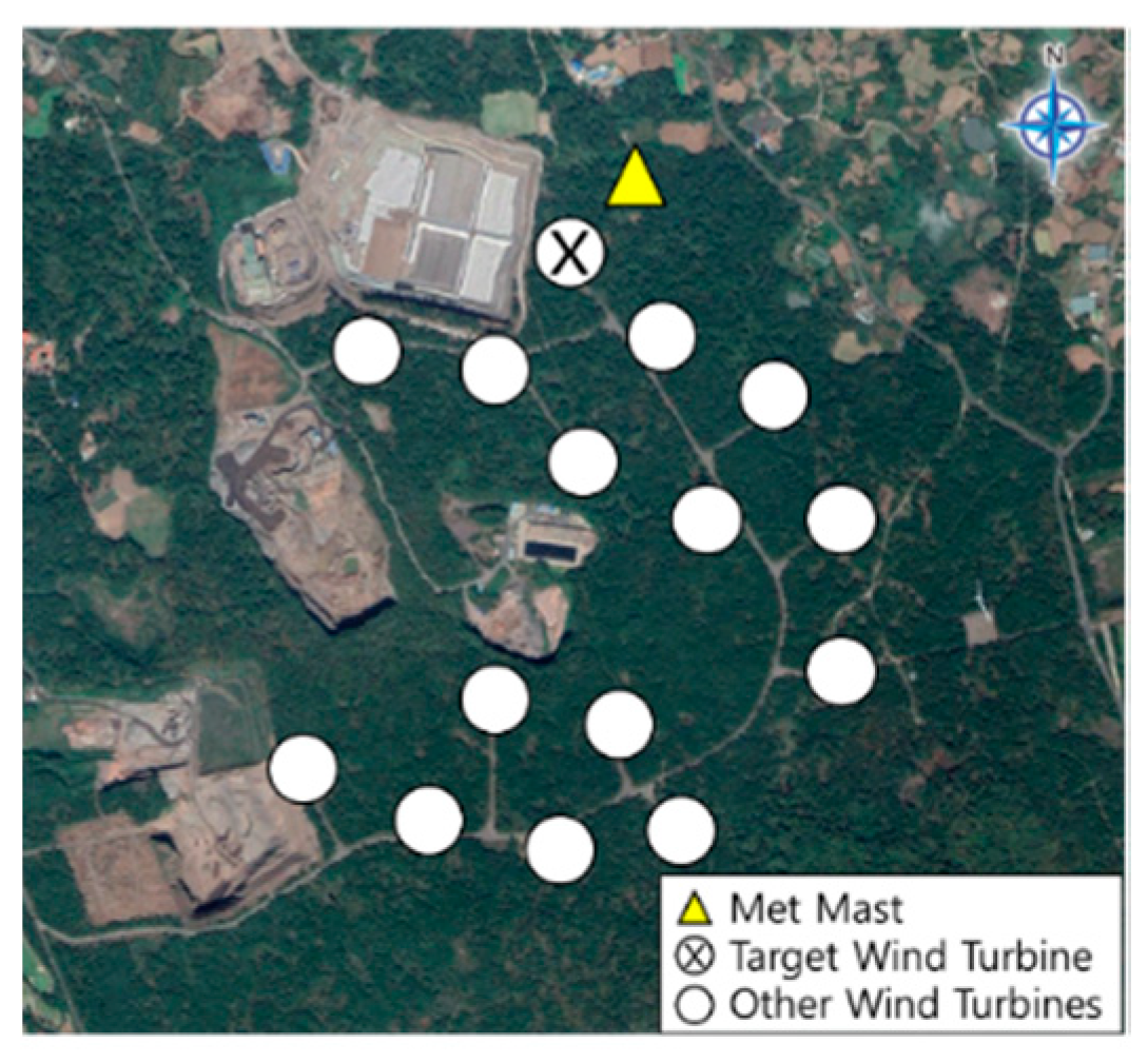
In this study, a wind turbine in a commercial wind farm D in South Korea was used as a target wind turbine. As shown in Figure 1, wind farm D consists of 15 wind turbines. The met mast is at the north of the target wind farm. The target wind turbine is about 2.5 RD (Rotor Diameter) away from the met mast, which corresponds to 220 m in distance. The met mast and the target wind turbine are located in a relatively flat terrain, and they are about 1.7 km away from the sea.
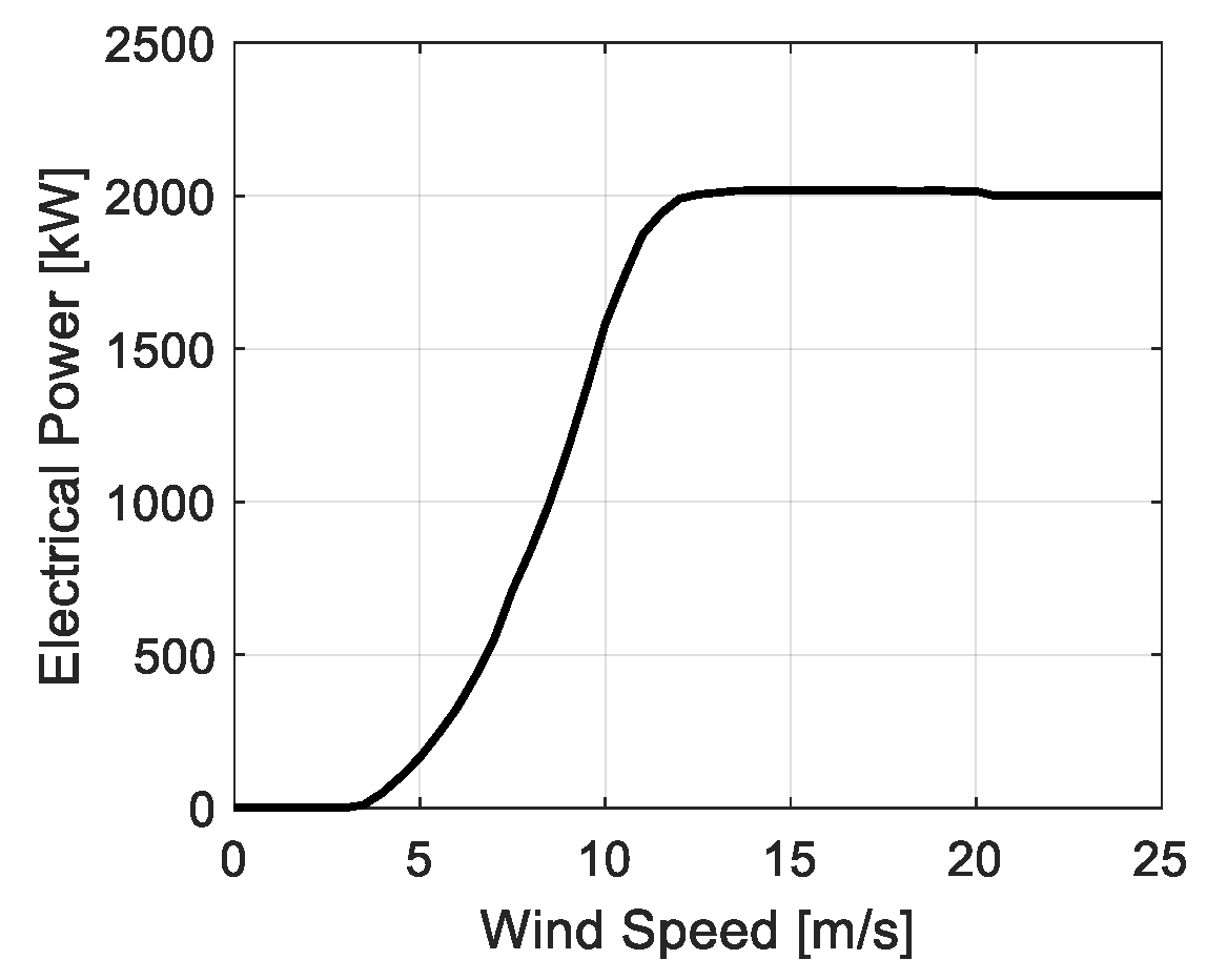
Table 1 shows the general specification of the target wind turbine. As shown in the table, the hub height of the wind turbine is 80 m. The cut-in, rated, cut-out wind speeds are 3.5 m/s, 12 m/s, and 25 m/s, respectively. Figure 2 shows the power curve showing the power output with respect to the wind speed for the standard air density, which is 1.225 kg/m3.
2.2. Wind Data
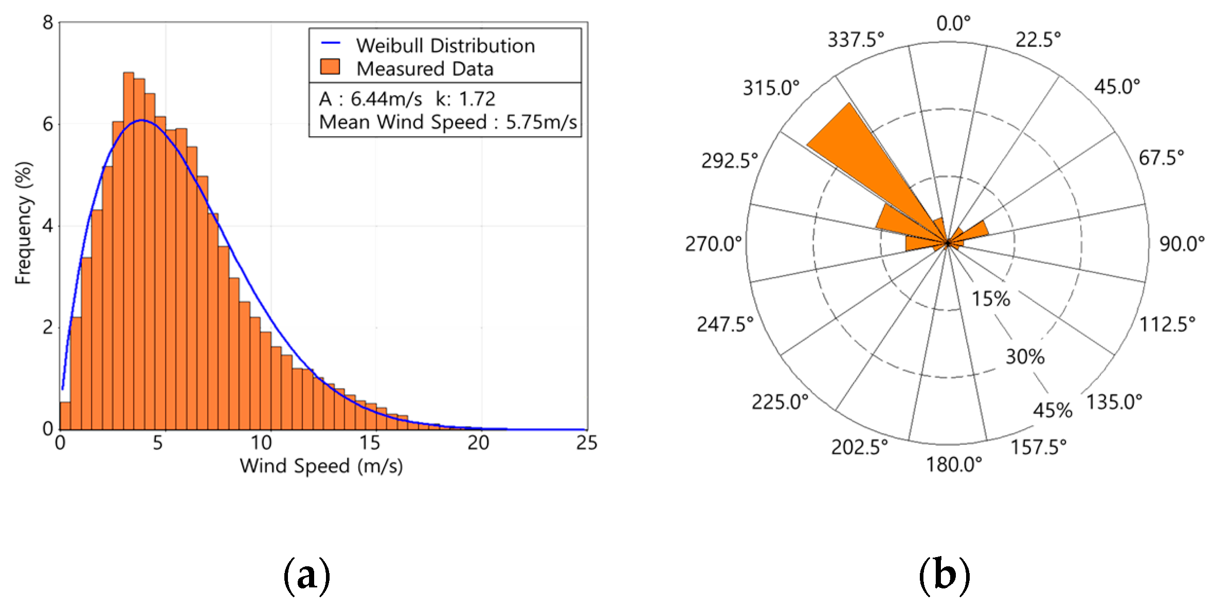
In this study, the 10-min averaged data measured from 1 January 2017 to 31 December 2017 at the meteorological mast were used. The meteorological mast sensors comprise anemometers, wind direction vanes, a temperature sensor, a barometric pressure sensor, and a relative humidity sensor. The anemometers were installed at heights of 80 m, 78 m, and 40 m. The wind direction vanes were installed at heights of 78 m and 40 m. The temperature sensor, barometric pressure sensor, and relative humidity sensor were installed at a height of 75 m. The data measured with the 80 m anemometer and 78 m wind direction vane were used to predict the electrical power production of the target wind turbine in the wind farm. Figure 3a shows the Weibull distribution, and Figure 3b is the wind energy rose obtained using the met mast data. As shown in Figure 3, the average wind speed at a height of 80 m is 5.75 m/s, and the prevailing wind direction is 315 degrees in 16 sector-wise angles.
According to the equation for data normalization provided by the International Electrotechnical Commission (IEC) standards 61400-12-1 2nd edition [16], the air density at the target wind turbine can be calculated using the measured 10-min average data for temperature and air pressure of the mast at a height of 75 m. The 10-min average air density was calculated using Equation (1):
In the equation, is the calculated 10-min average air density, is the measured 10-min average air pressure, is the measured 10-min average air temperature, and is the gas constant of dry air, which is 287.05 J/(kg·K). The air density calculated at a height of 75 m at the met mast position is 1.076 kg/m3. The air density for the target wind turbine was assumed to be the same as the air density at the met mast.
2.3. Terrain Modeling
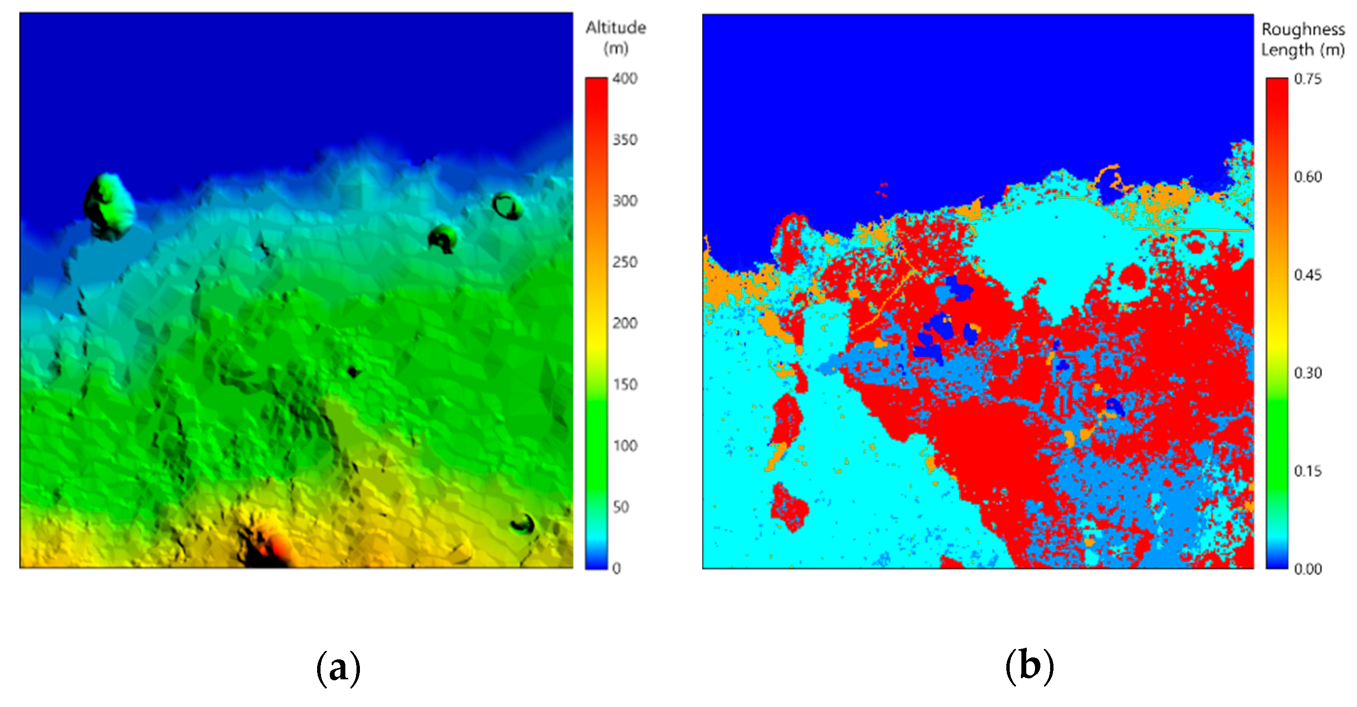
A terrain model that includes the information on both the topology and roughness was used for the CFD simulation analysis of the wind farm. The height contour map provided by the Korea National Spatial Information Portal and the land cover data provided by the Korea Ministry of Environment [17,18] were used to construct the terrain model.
The terrain model of the target wind farm was constructed by the geographic information system (GIS) software Global Mapper based on the height contour and the land cover data and implemented with the CFD simulation program, WindSim. Figure 4a,b shows the elevation and the roughness length information of the terrain model.
The size and grid spacing of the terrain model has an impact on the prediction results of the power output [19]. Therefore, in this study, the size of the terrain model was determined to be 10 km by 10 km, and the horizontal grid spacing was 25 m by 25 m. The number of vertical grids was 40, and the number of grids below the wind turbine hub height was six, to accurately simulate the wind characteristics in the wind farm.
The wind field analysis was carried out using WindSim based on the Reynolds-Averaged Navier–Stokes (RANS) equation. Because the equation is nonlinear, the solution is solved with the use of multiple iterations until convergence is obtained [20]. This study uses the GCV (Convergence control with new solver) solver in the CFD simulation WindSim to solve the RANS equation. The GCV method uses a pressure-based separation solver strategy to control the mass flux on the control-volume faces, providing faster convergence [21]. It was assumed that the atmospheric boundary layer had a height of 500 m, that the atmospheric flow was stable, and that the wind speed above 500 m was constant with height [22]. The boundary condition at the top was “fixed pressure”. The turbulence model used was the standard k-ε eddy viscosity turbulence model without considering temperature changes, where k is the turbulent flow energy and ε is the rate of turbulent dissipation.
Based on the results of the wind field analysis and the N.O. Jensen wake model [23], the 10-min averaged wind speed, wind direction, and electrical power of the target wind turbine were obtained from WindSim.
2.4. The Wind Turbine Matlab/Simulink Dynamic Model with a Wind Turbine Controller
In this study, the dynamic simulation model of a wind turbine was used for the prediction of the electrical power production by the target wind turbine. The model was developed in the previous study and modified for this study to be used to predict the power of an actual wind turbine [15].
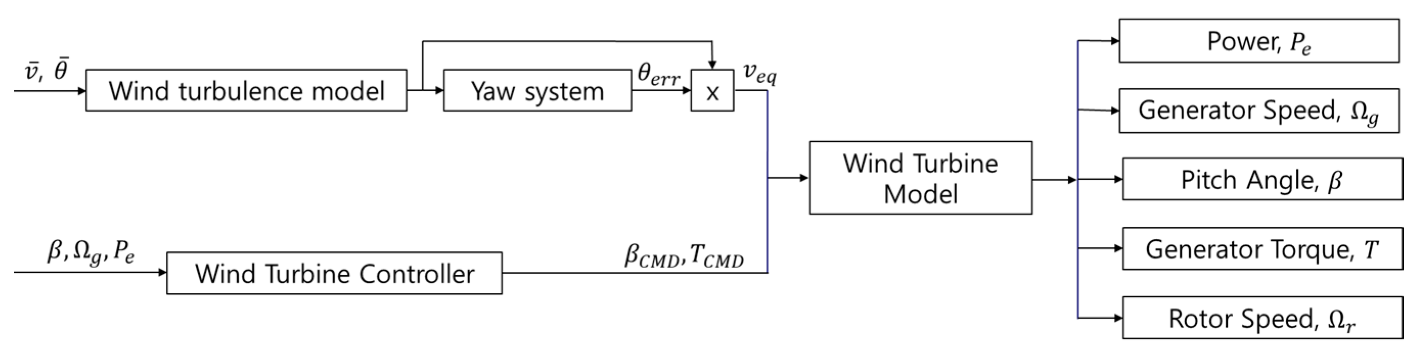
Figure 5 shows the schematic of the dynamic model used for the target wind turbine. The dynamic model of the wind turbine is composed of four parts: the wind turbulence model, the yaw system model, the wind turbine controller, and the wind turbine model. The model requires 10-min average wind speed and direction data together with their standard deviations as inputs and calculates the electrical power output of the wind turbine with the power and yaw control algorithms. Detailed information on the model is available in Ref. [15].
2.4.1. The Wind Turbine Matlab/Simulink Dynamic Model
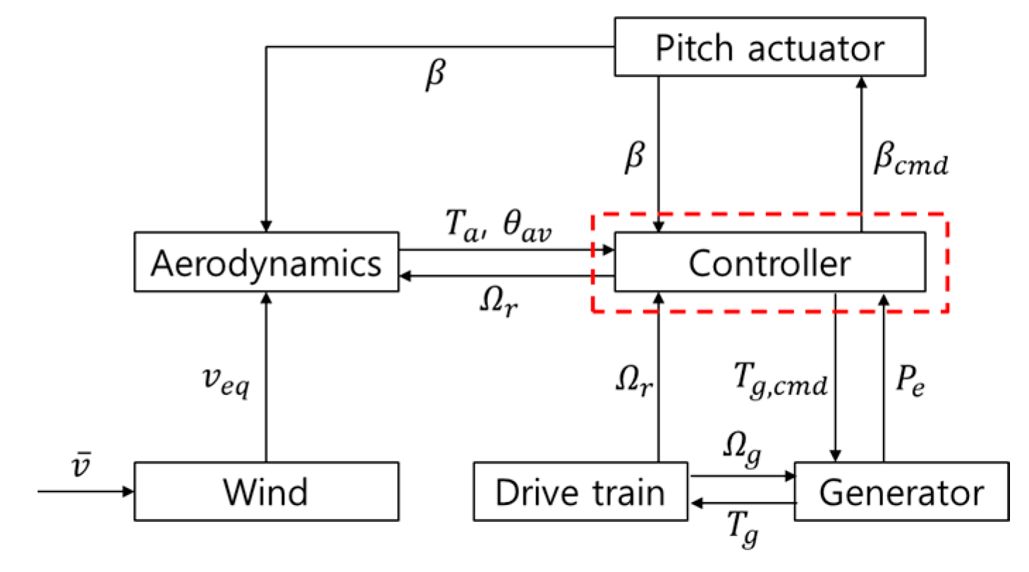
In this study, the wind turbine dynamic model was simulated by using Matlab/Simulink, and the block diagram of the dynamic wind turbine model is shown in Figure 6. As shown in the figure, the wind turbine dynamic model is composed of the aerodynamics model, the drive train model, the generator model, the pitch actuator model, and the control system model.
The aerodynamic power can be simply modeled using Equation (2).
where is the aerodynamics power of the wind turbine, is the air density, is the wind turbine radius, is the wind speed, and is the power coefficient of the wind turbine which depends on the tip speed ratio and the blade pitch angle . The power coefficients for various tip speed ratios and blade pitch angles are calculated from a BEMT (Blade Element Momentum Theory) software such as Bladed and used as a look-up table in the aerodynamics model.
The drive train model is composed of a low-speed shaft, a gearbox, and a high-speed shaft. The aerodynamics torque and generator torque are the inputs of the drive train model. The low-speed shaft and high-speed shaft can be modeled by the inertia, the stiffness, and the damping. The drive train model was simulated using Equations (3) and (4). The relationship between the low-speed shaft and the high-speed shaft is shown in Equation (5) [24].
where is the inertia, is the rotation speed, is the torque, is the torsional stiffness, is the torsional damping, is the rotation angle, is the damping, and is the gear ratio. Moreover, represents the aerodynamic, and mean the rotor and the generator, respectively.
The pitch actuator and the generator were modeled as 1st-order systems, which are shown in Equations (6) and (7), respectively [25].
In Equations (6) and (7), is the pitch angle, is the pitch angle command, and is the time constant of the pitch actuator. is the generator torque, is the generator torque command, and is the time constant of the generator torque.
2.4.2. The Wind Turbine Control System
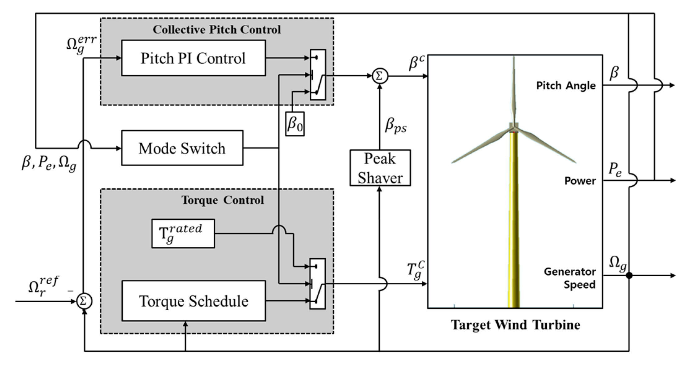
Figure 7 shows the wind turbine controller used in the dynamic wind turbine model. It consists of a basic torque and blade pitch control for power maximization and regulation and a peak shaving to use blade pitching to reduce thrust force by sacrificing power slightly near the rated wind speed region [26].
To maximize the electrical power of the wind turbine in regions where the wind speed is lower than the rated wind speed, the pitch angle of the blade is fixed to be the fine pitch angle, and the optimal torque command is sent to the generator to maximize the power coefficient of the rotor [27]. To maintain the rated electrical power of the wind turbine in regions where the wind speed is higher than the rated wind speed, the torque is fixed to be the rated torque, and the blade pitch angle of the wind turbine is adjusted to keep the rated rotational speed of the rotor. The torque control algorithm in the control system used was a simple open-loop control using a look-up table with an input of measured generator speed and output of optimal generator torque. Moreover, the blade pitch control in the control system used the classical proportional–integral (PI) algorithm to minimize the error between the measured generator speed and the rated value.
2.5. Conversion of Power Curve to Include Air Density Effect
The power coefficient curve and thrust coefficient curve used for the wind turbine dynamic model are derived from Bladed under the condition of a standard air density of 1.225 kg/m3. However, the actual air density of a wind farm is different from the standard value, which causes a discrepancy between the prediction and the measured power output.
In this study, a novel method is proposed to match the power of a dynamic wind turbine model with that of a wind turbine with actual air density by tuning the controller. The first step of this method is to convert the power curve of the wind turbine based on the standard air density to that based on the actual mean air density of the site. This conversion is possible by using the correction method for wind turbines with active power control described in the standard, IEC 61400-12-1 [16].
Equation (8) represents the wind speed correction equation calculated based on the IEC standard.
In Equation (8), is the measured wind speed averaged over 10 min, is the normalized wind speed, is the derived 10-min average air density, and is the reference air density, known to be 1.225 kg/m3. Through Equation (8), the wind speed of a power curve is converted to consider the mean air density at the site.
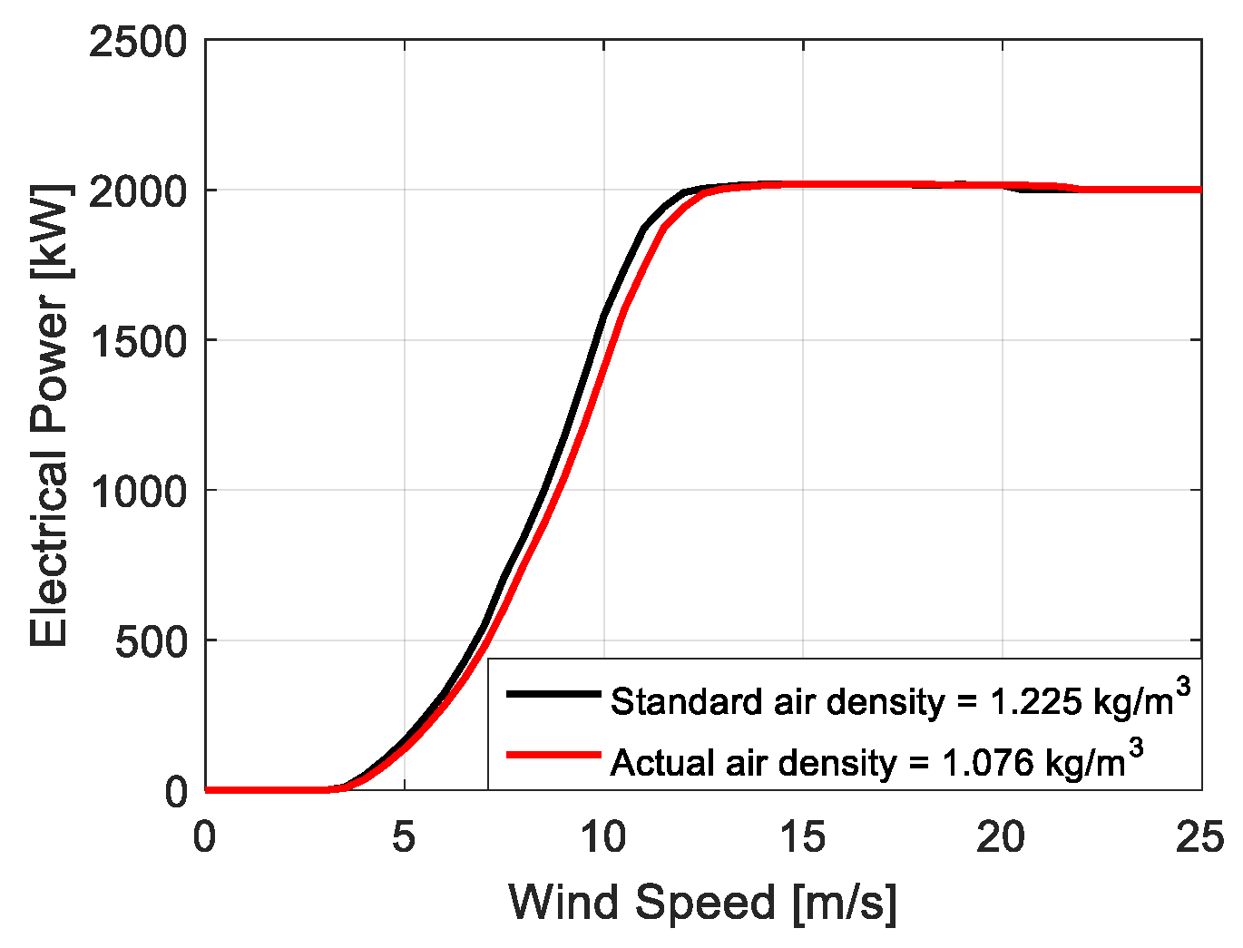
Figure 8 shows the comparison between the power curve with the standard air density and the power curve with the actual mean air density. It can be seen from the figure that when the power is lower than the rated power, the power with the standard air density is slightly higher than that with the actual mean air density.
2.6. Tuning of the Wind Turbine Controller to Consider Actual Mean Air Density
To consider the actual mean air density of the site in the dynamic model, the wind turbine controller needs to be tuned by considering the power curve with the actual mean air density as a target.
In the torque control region where the wind speed is lower than 10 m/s, the look-up table of the torque scheduling was tuned so that the power curve of the dynamic model is matched with the power curve with the actual mean air density. In the transition region where the wind speed is higher than 10 m/s and lower than the rated wind speed, the peak shaving algorithm and torque scheduling were used to match the target power curve. For the rated power region, the closed-loop PI control strategy was used, and no tuning was necessary because the algorithm is not affected by the change of air density.
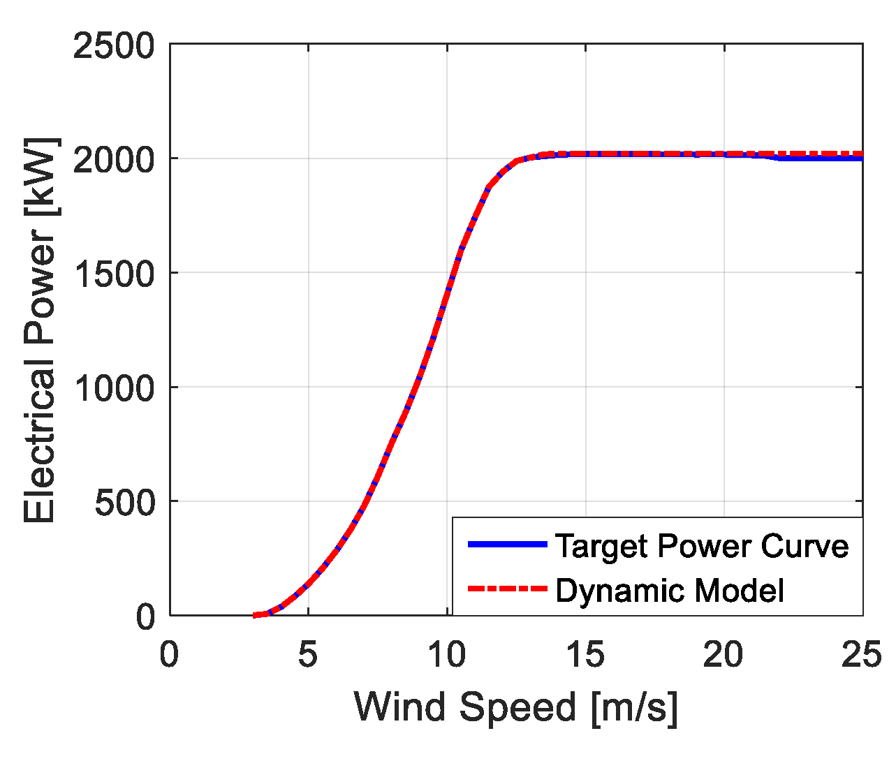
Figure 9 compares the target power curve with the power curve obtained from the dynamic model after tuning the control algorithms. The two power curves are well matched.
3. Results
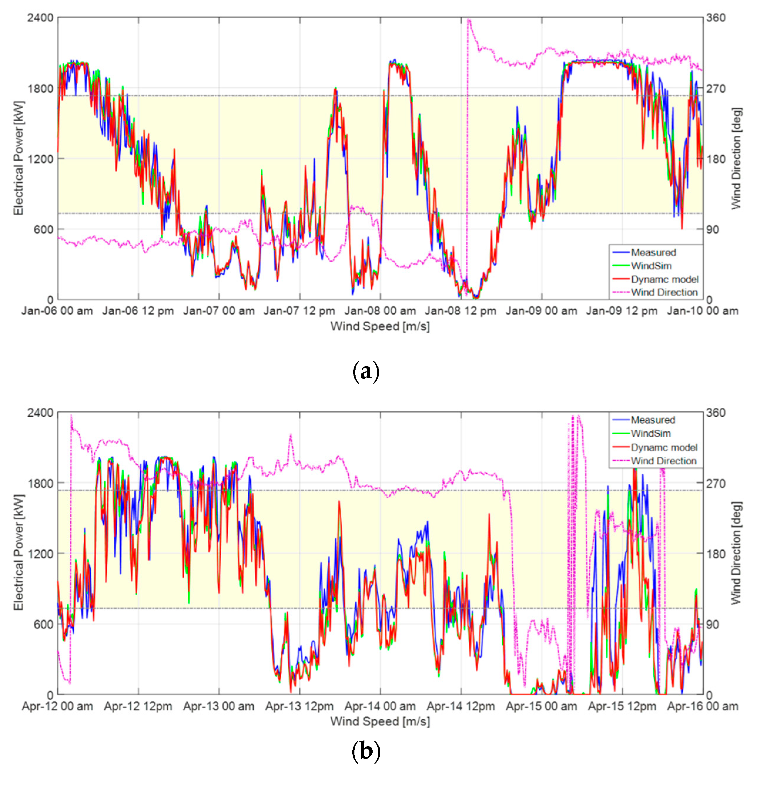
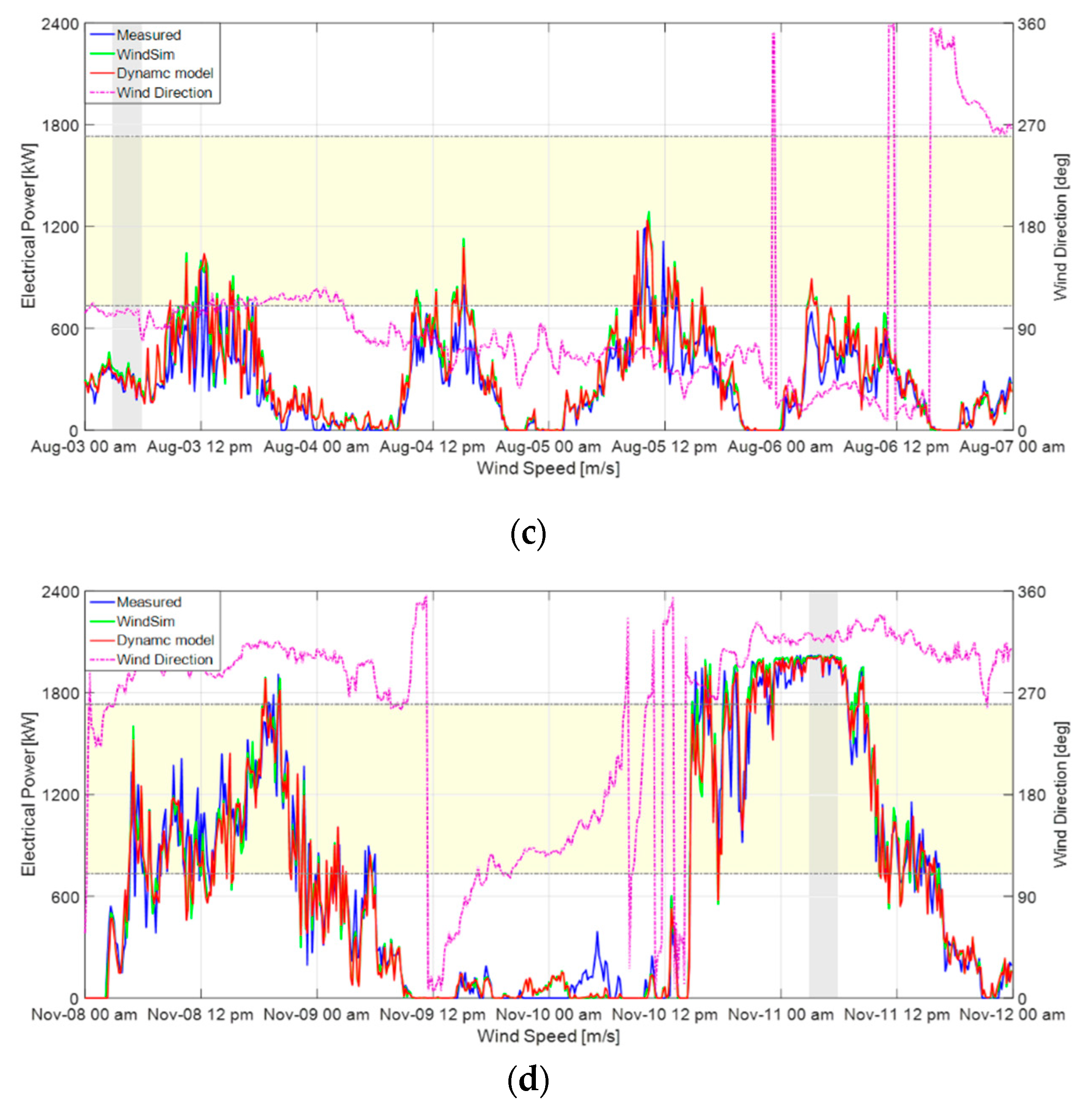
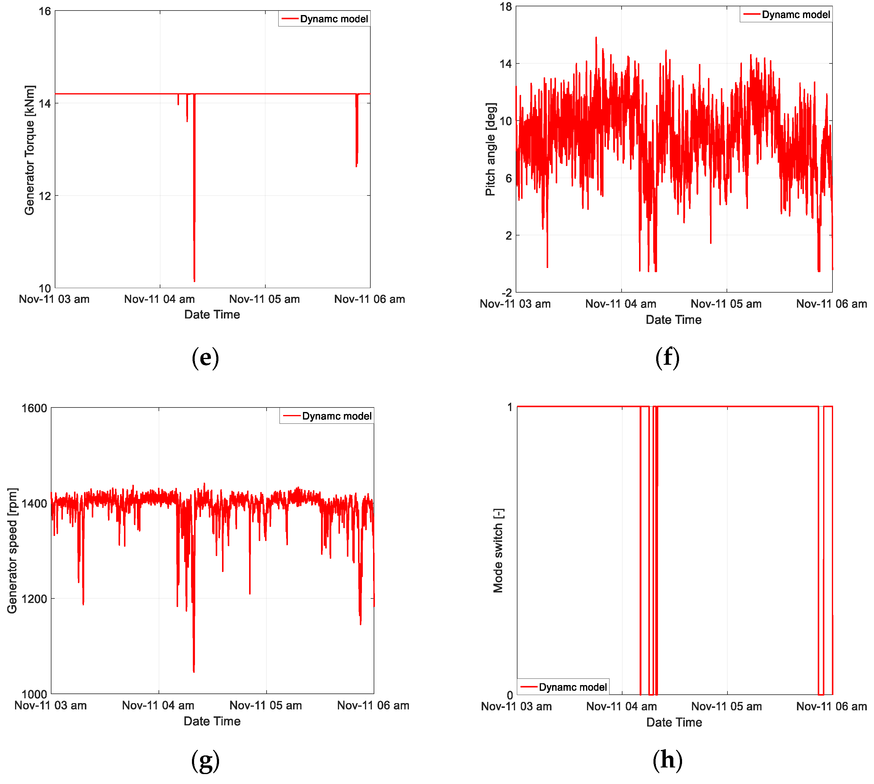
Figure 10a–d shows the results of the comparison between the measured electrical power, the electrical power predicted by WindSim, and the electrical power predicted by the dynamic model for four days in January, April, August, and November, respectively. The wind direction data measured from the met mast are also shown in the figure. The measured data and the data obtained from WindSim were 10-min averaged data, and therefore, the data from the dynamic model, which was originally in 1-s intervals, were converted to 10 min averaged data.
As shown in the figure, both predictions by WindSim and the dynamic model were close to the measured power; however, there are regions where relatively large discrepancies exist in Figure 10b,d. For these regions, the wind directions are between 110 degrees and 260 degrees. The reason for these relatively large discrepancies in these regions is that the met mast is located within the wake region of the wind turbines around the target wind turbine for those wind directions, and the wind speed implemented with WindSim to predict the wind speed for the target wind turbine is the wind speed reduced by the wake effect. To obtain the wind speed for the target wind turbine, WindSim again applies a wake model in the case where the wind direction corresponds to the direction causing the wake effect on the target wind turbine. Therefore, the wind speed obtained for the target wind turbine from WindSim in those wind directions becomes lower than the actual wind speed of the target wind turbine and the power output predicted by WindSim and the dynamic model becomes lower than the measured power.
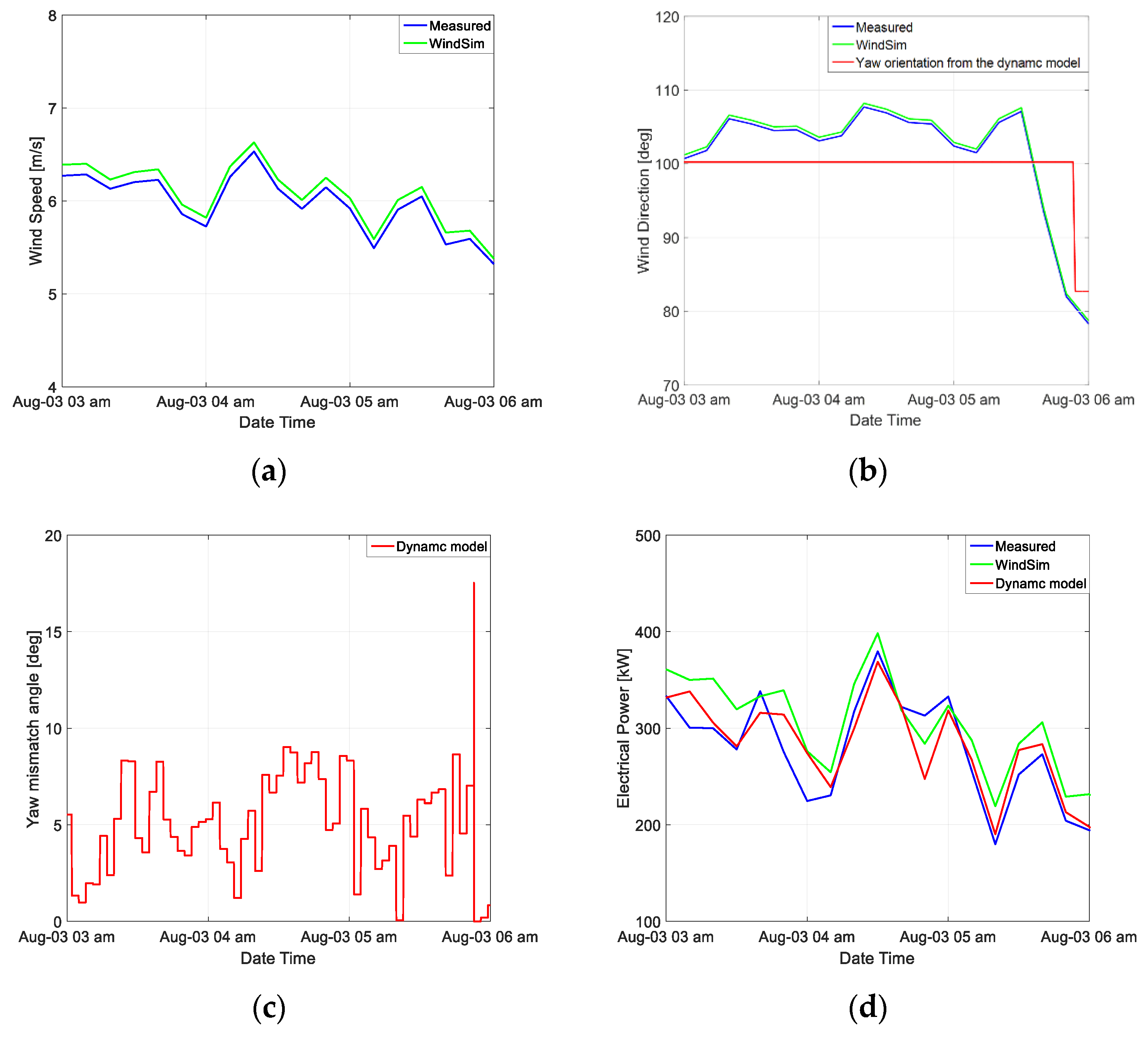
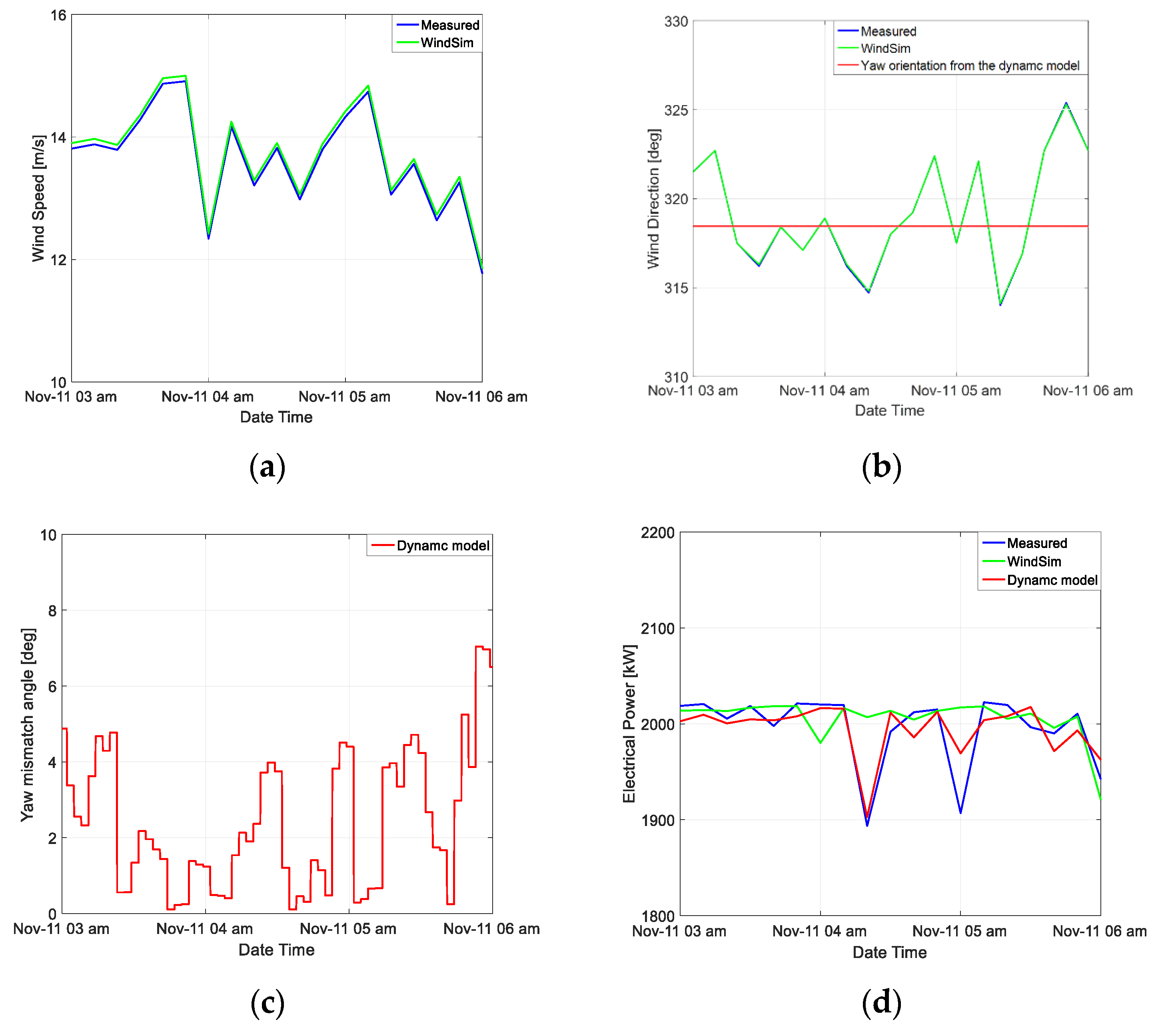
To compare the results in more detail, small portions of Figure 10c,d corresponding to three hours are replotted in Figure 11 and Figure 12, respectively. Figure 11 shows a mean wind speed lower than the rated wind speed, and Figure 12 shows a mean wind speed higher than the rated value. Figure 11a and Figure 12a show the wind speed measured from the met mast and the wind speed of the target wind turbine predicted by WindSim. For both cases, the wind speed of the target wind turbine predicted by WindSim is slightly higher than the wind speed measured from a nearby met mast. This is partly due to the fact that the altitude of the target wind turbine location is slightly higher than that of the met mast location.
Figure 11b and Figure 12b show the wind direction measured from the met mast and the wind direction at the wind turbine position predicted by WindSim. The wind direction of the target wind turbine predicted by WindSim is basically consistent with the measured wind direction. They also show the turbine orientation predicted by the dynamic model. In Figure 11b, the yaw mismatch angle exceeded 11 degrees in the end, and the yaw system was activated to reduce the mismatch angle. In Figure 12b, the yaw orientation did not change because of the small yaw mismatch angles compared with the threshold. These are also shown in Figure 11c and Figure 12c, which show the yaw mismatch angles. The mismatch angles are three-minute averaged values.
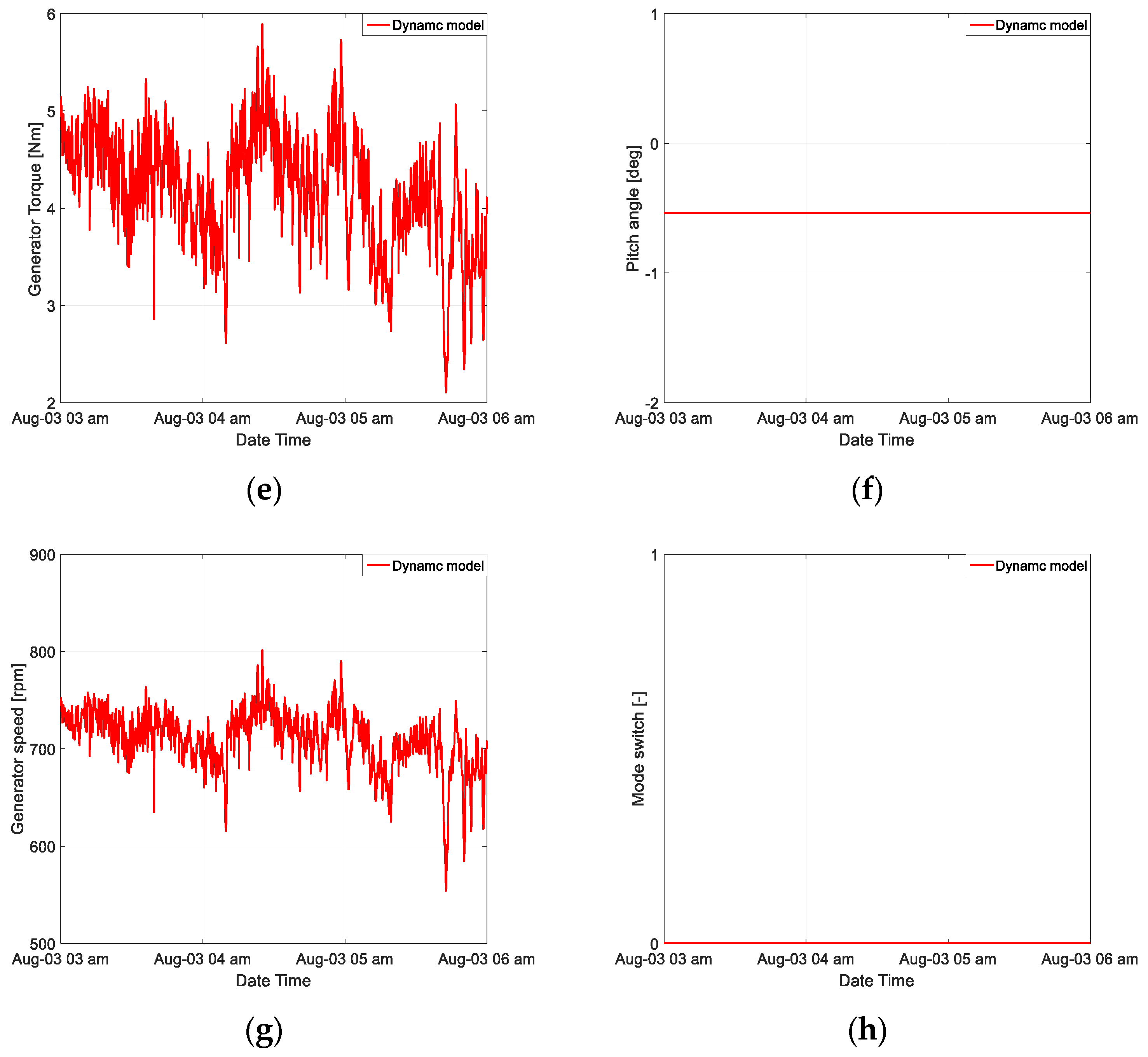
Figure 11d and Figure 12d show the measured electrical power, the electrical power predicted by WindSim, and the electrical power predicted by the dynamic model. Figure 11d shows the electrical power when the wind speed is lower than the rated wind speed. Therefore, the blade pitch angle is fixed to be the fine pitch, and the generator torque is adjusted to maximize the power coefficient. As shown in the figure, the power prediction from WindSim consistently overestimates the measured power. The power predicted by the dynamic model looks similar to the WindSim results but closer to the measured power. The generator torque and the blade pitch angle from the dynamic model is shown in Figure 11e,f. Figure 12d shows the electrical power when the wind speed is mostly higher than the rated wind speed. Therefore, the generator torque is fixed to the rated value, and the blade pitch angle is adjusted to maintain the rated wind speed and the rated power. Figure 12e,f shows the generator torque and the blade pitch angle from the dynamic model. In Figure 12d, there are a few downward spikes in the measured power. The dynamic model shows similar downward spikes but the power from WindSim does not. The reason for this is that WindSim does not consider wind turbine dynamics and yaw mismatch, and the power is solely dependent on the wind speed. Based on Figure 12a, the wind speed is maintained to be mostly higher than the rated wind speed, and therefore, the power prediction from WindSim is mostly close to the rated power. However, if we look at the results from the dynamic model in Figure 12e,h, the mode switch was turned off a few times between 4:00 and 5:00 o’clock, and the generator torque was reduced. As a result, the power decreased as a downward spike. The dynamic model includes wind turbine dynamics and could show similar measured power variations.
Figure 11g and Figure 12g show the generator speed obtained from the dynamic model. For Figure 11g, the generator speed varies between 550 rpm and 800 rpm to maximize the power coefficient; on the other hand, for Figure 12g, the generator speed is generally close to the rated value, which is about 1400 rpm.
Table 2 shows the relative percentage errors of the electrical energy production with respect to the measure values given in Figure 11d and Figure 12d. As shown in the table, the relative errors of the energy production predicted by WindSim and the dynamic model for Figure 11d are 9.45% and 1.12%, respectively, which is the case when the wind speed is lower than the rated wind speed. The errors are reduced to 0.48% and −0.06%, respectively, for Figure 12d in which the wind speed is higher than the rated wind speed. For both cases, the errors from the dynamic model are smaller than those from WindSim, because the dynamic model considers the wind turbine dynamics and the yaw motion. In Table 2, the electrical energy production was normalized by the measured electrical energy production (MWh) of the corresponding period, respectively.
Table 3 shows the comparison between the measured AEP, the AEP predicted by the WindSim, and the AEP predicted by the dynamic model with and without yaw motion for the target wind turbine. As shown in the table, the relative error of AEP predicted by WindSim is 2.75%, and those of the dynamic model without and with the yaw system are 2.11% and 0.16%, respectively. Based on the results, the prediction error from ignoring yaw mismatch errors is larger than the prediction error from ignoring wind turbine dynamics. The annual energy production from the dynamic model is also about 2.52% smaller than that from WindSim. This result is similar to the result in Ref. [15], where the relative differences between WindPRO and the dynamic model for four different sites with the NREL 5 MW wind turbine were between 0.83% and 4.91%. In Table 3, the AEP is normalized by the measured AEP (MWh) for one year.
4. Conclusions
In this study, a dynamic wind turbine model was constructed for an actual 2 MW wind turbine, and the wind turbine performance was predicted and validated experimentally. The dynamic model was constructed using Matlab/Simulink to consider the wind turbine dynamics, including yaw systems and a wind turbine controller using basic torque and pitch control algorithms with peak shaving in the transition from maximum power point tracking to the rated power regions. In addition, to consider the density effect of the test site, the torque scheduling and the peak shaving were tuned to reproduce the power curve with the actual mean air density.
For experimental validation, the AEP predicted by the dynamic model was compared with that by WindSim and the measured power. As the result, the relative error of WindSim was 2.75%, and those of the dynamic model without and with yaw were 2.11% and 0.16%, respectively. Although the results are only for a single wind turbine case, the prediction of AEP from the dynamic model was found to be accurate. However, further research is needed for different wind turbines and sites to better understand the performance of the dynamic simulation model.
Author Contributions
Y.S. performed the simulation of the wind turbine, analyzed the results, and wrote the paper. I.P. supervised the research, analyzed the results, and revised the paper. All authors have read and agreed to the published version of the manuscript.
Funding
This work was supported by the Human Resources Program in Energy Technology and the New and Renewable Energy-Core Technology Program of the Korea Institute of Energy Technology Evaluation and Planning (KETEP) with a granted financial resource from the Ministry of Trade, Industry and Energy, Republic of Korea (Grants No. 20173010025010 and 20204030200010).
Acknowledgments
The authors would like to acknowledge the support from Han Jin Ind. Co. Ltd. for the wind turbine model construction. The authors would also like to acknowledge the support from Jeju Energy Corp. for the climatology data of the site.
Conflicts of Interest
The authors declare no conflict of interest.
References
- “Renewable energy 3020” Implementation Plan. Available online: http://www.motie.go.kr/motiee/presse/press2/bbs/bbsView.do?bbs_seq_n=159996&bbs_cd_n=81 (accessed on 3 August 2020). (In Korean)
- South Korea Wind Turbine Installation Status. Available online: http://kweia.or.kr/bbs/board.php?bo_table=sub03_03 (accessed on 3 August 2020). (In Korean).
- Yue, C.; Liu, C.; Tu, C.; Lin, T. Prediction of Power Generation by Offshore Wind Farms Using Multiple Data Sources. Energies 2019, 12, 700. [Google Scholar] [CrossRef] [Green Version]
- Song, Y.; Kwon, I.; Paek, I. Investigation on promising offshore wind farm sites and their wind farm capacity factors considering wake losses in Korea. J. Wind Energy 2018, 9, 27–36. [Google Scholar] [CrossRef]
- Park, U.; Yoo, N.; Kim, J.; Kim, K.; Min, D.; Lee, S.; Paek, I.; Kim, H. The selection of promising wind farm sites in Gangwon province using multi exclusion analysis. J. Korean Sol. Energy Soc. 2015, 35, 1–10. [Google Scholar] [CrossRef] [Green Version]
- Dhunny, A.; Lollchund, M.; Rughooputh, S. Wind energy evaluation for a highly complex terrain using Computational Fluid Dynamics (CFD). Renew. Energy 2017, 101, 1–9. [Google Scholar] [CrossRef]
- Song, Y.; Kim, H.; Byeon, J.; Paek, I.; Yoo, N. A Feasibility Study on Annual Energy Production of the Offshore Wind Farm using MERRA Reanalysis Data. J. Korean Sol. Energy Soc. 2015, 35, 33–41. [Google Scholar] [CrossRef] [Green Version]
- Kim, J.; Kwon, I.; Park, U.; Paek, I.; Yoo, N. Prediction of Annual Energy Production of Wind Farms in Complex Terrain using MERRA Reanalysis Data. J. Korean Sol. Energy Soc. 2014, 34, 82–90. [Google Scholar] [CrossRef] [Green Version]
- Tabas, D.; Fang, J.; Porté-Agel, F. Wind Energy Prediction in Highly Complex Terrain by Computational Fluid Dynamics. Energies 2019, 12, 1311. [Google Scholar] [CrossRef] [Green Version]
- Kim, H.; Song, Y.; Paek, I. Predicted and Validation of Annual Energy Production of Garyeok-do Wind Farm in Saemangeu Area. J. Wind Energy 2018, 9, 19–24. [Google Scholar]
- Kim, H.; Kim, K.; Paek, I. Power regulation of upstream wind turbines for power increase in a wind farm. Int. J. Precis. Eng. Manuf. 2016, 17, 665–670. [Google Scholar] [CrossRef]
- Kim, H.; Kim, K.; Paek, I. Model Based Open-Loop Wind Farm Control Using Active Power for Power Increase and Load Reduction. Appl. Sci. 2017, 7, 1068. [Google Scholar] [CrossRef] [Green Version]
- Kim, H.; Kim, K.; Paek, I. A Study on the Effect of Closed-Loop Wind Farm Control on Power and Tower Load in Derating the TSO Command Condition. Energies 2019, 12, 2004. [Google Scholar] [CrossRef] [Green Version]
- Campagnolo, F.; Weber, R.; Schreiber, J.; Bottasso, C. Wind tunnel testing of wake steering with dynamic wind direction changes. Wind Energy Sci. 2020, 5, 1273–1295. [Google Scholar] [CrossRef]
- Kim, K.; Lim, C.; Oh, Y.; Kwon, I.; Yoo, N.; Paek, I. Time-domain dynamic simulation of a wind turbine including yaw motion for power prediction. Int. J. Precis. Eng. Manuf. 2014, 15, 2199–2203. [Google Scholar] [CrossRef]
- International Electrotechnical Commission (IEC). Wind Turbine Generator Systems Part 12-1: Power Performance Measurements of Electricity Producing Wind Turbines, 2nd ed.; International Electrotechnical Commission (IEC): Geneva, Switzerland, 2017. [Google Scholar]
- Ministry of Land. Infrastructure and Transport, National Spatial Data Infrastructure Portal. Available online: http://www.nsdi.go.kr/lxportal/?menuno=2679 (accessed on 3 August 2020).
- Ministry of Environment. Environmental Spatial Information Service. Available online: http://egis.me.go.kr/map/map.do?type=land (accessed on 3 August 2020).
- Hwang, Y.; Paek, I.; Yoon, K.; Lee, W.; Yoo, N.; Nam, Y. Application of wind data from automated weather stations to wind resources estimation in Korea. J. Mech. Sci. Technol. 2010, 24, 2017–2023. [Google Scholar] [CrossRef]
- WindSim AS. Available online: https://www.windsim.com (accessed on 3 August 2020).
- Cham. The Phoenics Encyclopedia. Available online: http://www.cham.co.uk/phoenics/d_polis/d_enc/enc_gcv.htm (accessed on 3 August 2020).
- Fallo, D. Wind Energy Resource Evaluation in a Site of Central Italy by CFD Simulations. Ph.D. Thesis, University of Cagliari, Cagliari, Italy, 2007. [Google Scholar]
- Katic, I.; Højstrup, J.; Jensen, N. A simple model for cluster efficiency. In Proceedings of the European Wind Energy Association Conference and Exhibition, Roma, Italy, 7–9 October 1986; Volume 1, pp. 407–410. [Google Scholar]
- Nam, Y.; Kim, J.; Paek, I.; Moon, Y.; Kim, S.; Kim, D. Feedforward Pitch Control Using Wind Speed Estimation. J. Power Electron. 2011, 11, 211–217. [Google Scholar] [CrossRef]
- Bianchi, F.; de Battista, H.; Mantz, R. Wind Turbine Control Systems, Principles, Modelling and Gain Scheduling Design. Available online: https://0-www-springer-com.brum.beds.ac.uk/gp/book/9781846284922 (accessed on 3 August 2020).
- Kim, K.; Kim, H.; Paek, I. Application and Validation of Peak Shaving to Improve Performance of a 100 kW Wind Turbine. Int. J. Precis. Eng. Manuf.-Green Tech. 2020, 7, 411–421. [Google Scholar] [CrossRef]
- Jonkman, J.; Butterfield, S.; Musial, W.; Scott, G. Definition of a 5-MW Reference Wind Turbine for Offshore System Development; National Renewable Energy Lab. (NREL): Golden, CO, USA, 2009; p. 947422.
Figure 1.
The layout of wind farm D (Source: Google Maps).

Figure 2.
The power curve of the target wind turbine.

Figure 3.
Measured wind data for the target wind turbine: (a) Weibull distribution; (b) total wind energy rose.
Figure 3.
Measured wind data for the target wind turbine: (a) Weibull distribution; (b) total wind energy rose.

Figure 4.
Terrain model of the target wind farm L (a) elevation; (b) roughness length.

Figure 5.
The wind turbine dynamic model.

Figure 6.
The block diagram of the wind turbine model.

Figure 7.
The wind turbine model control system.

Figure 8.
Comparison of the power curve of standard air density and the power curve of actual air density.
Figure 8.
Comparison of the power curve of standard air density and the power curve of actual air density.

Figure 9.
Comparison of the measured power curve report and the power curve of different controllers at 1.076 kg/m3.
Figure 9.
Comparison of the measured power curve report and the power curve of different controllers at 1.076 kg/m3.

Figure 10.
Comparison of the measured and predicted electrical power: (a) January, (b) April, (c) August, (d) November.
Figure 10.
Comparison of the measured and predicted electrical power: (a) January, (b) April, (c) August, (d) November.


Figure 11.
Comparison of the measured and predicted data for 3 h in August: (a) wind speed, (b) wind direction, (c) yaw mismatch, (d) electrical power, (e) generator torque, (f) pitch angle, (g) generator speed, (h) model switch.
Figure 11.
Comparison of the measured and predicted data for 3 h in August: (a) wind speed, (b) wind direction, (c) yaw mismatch, (d) electrical power, (e) generator torque, (f) pitch angle, (g) generator speed, (h) model switch.


Figure 12.
Comparison of the measured and predicted data for 3 h in November (a) wind speed, (b) wind direction, (c) yaw mismatch, (d) electrical power, (e) generator torque, (f) pitch angle, (g) generator speed, (h) model switch.
Figure 12.
Comparison of the measured and predicted data for 3 h in November (a) wind speed, (b) wind direction, (c) yaw mismatch, (d) electrical power, (e) generator torque, (f) pitch angle, (g) generator speed, (h) model switch.


Table 1.
General specification of the target wind turbine.
| Properties | Value |
|---|---|
| Rated power | 2 MW |
| Cut-in, rated, cut-out Wind speed | 3.5 m/s, 12 m/s, 25 m/s |
| Hub height | 80 m |
| Power control | Pitch Control |
Table 2.
Relative errors of electrical energy production prediction for the data shown in Figure 10d and Figure 11d.
| Normalized Measured | Normalized WindSim | Normalized Dynamic Model | |
|---|---|---|---|
| Electrical energy production for Figure 10d | 1.0000 | 1.0945 | 1.0112 |
| Electrical energy production for Figure 11d | 1.0000 | 1.0048 | 0.9994 |
| Relative errors for Figure 10d | - | 9.45% | 1.12% |
| Relative errors for Figure 11d | - | 0.48% | −0.06% |
Table 3.
The relative errors of the annual energy production (AEP) by the measured and other models.
Table 3.
The relative errors of the annual energy production (AEP) by the measured and other models.
| Normalized Measured | Normalized WindSim | Normalized Dynamic Model without Yaw | Normalized Dynamic Model with Yaw | |
|---|---|---|---|---|
| AEP | 1.0000 | 1.0275 | 1.0211 | 1.0016 |
| Relative error | - | 2.75% | 2.11% | 0.16% |
Publisher’s Note: MDPI stays neutral with regard to jurisdictional claims in published maps and institutional affiliations. |
© 2020 by the authors. Licensee MDPI, Basel, Switzerland. This article is an open access article distributed under the terms and conditions of the Creative Commons Attribution (CC BY) license (http://creativecommons.org/licenses/by/4.0/).
Share and Cite
MDPI and ACS Style
Song, Y.; Paek, I. Prediction and Validation of the Annual Energy Production of a Wind Turbine Using WindSim and a Dynamic Wind Turbine Model. Energies 2020, 13, 6604. https://0-doi-org.brum.beds.ac.uk/10.3390/en13246604
AMA Style
Song Y, Paek I. Prediction and Validation of the Annual Energy Production of a Wind Turbine Using WindSim and a Dynamic Wind Turbine Model. Energies. 2020; 13(24):6604. https://0-doi-org.brum.beds.ac.uk/10.3390/en13246604
Chicago/Turabian StyleSong, Yuan, and Insu Paek. 2020. "Prediction and Validation of the Annual Energy Production of a Wind Turbine Using WindSim and a Dynamic Wind Turbine Model" Energies 13, no. 24: 6604. https://0-doi-org.brum.beds.ac.uk/10.3390/en13246604
Note that from the first issue of 2016, this journal uses article numbers instead of page numbers. See further details here.