Article

Assessment of the Condition of Pipelines Using Convolutional Neural Networks

1
Industrial heat power and heat supply systems, Kazan State Power Engineering University, Kazan 420066, Russia
2
Computer Systems, Kazan National Research Technical University named after A.N. Tupolev-KAI, Kazan 420111, Russia
*
Author to whom correspondence should be addressed.
Submission received: 31 December 2019 / Revised: 21 January 2020 / Accepted: 22 January 2020 / Published: 1 February 2020

Abstract

:
Pipelines are structural elements of many systems. For example, they are used in water supply and heat supply systems, in chemical production facilities, aircraft manufacturing, and in the oil and gas industry. Accidents in piping systems result in significant economic damage. An important factor for ensuring the reliability of energy transportation systems is the assessment of real technical conditions of pipelines. Methods for assessing the state of pipeline systems by their vibro-acoustic parameters are widely used today. Traditionally, the Fourier transform is used to process vibration signals. However, as a rule, the oscillations of the pipe-liquid system are non-linear and non-stationary. This reduces the reliability of devices based on the implementation of classical methods of analysis. The authors used neural network methods for the analysis of vibro-signals, which made it possible to increase the reliability of diagnosing pipeline systems. The present work considers a method of neural network analysis of amplitude-frequency measurements in pipelines to identify the presence of a defect and further clarify its variety.

1. Introduction

Pipelines are an important part of energy systems. Accidents in pipelines for heat and water supply occur periodically and quite often due to corrosion and cracking. According to some data, the number of accidents in the Russian Federation is 0.94–2.86 per 1 km of pipeline network (with a total length of 170,000 km in two-pipe terms). This is due to the lack of flaw detection control during construction and operation, as well as the means of electrochemical protection. As a result, in many cities in Russia, the resource of pipeline networks is 70–80% depleted, and a large number of leaks leads to excessive heat losses. According to some reports, the real heat loss of heating network pipelines in the Russian Federation is 324 million Gcal/year, which is about 16% of the heat supplied to consumers. Thus, in the existing heating networks, there are large reserves of saved thermal energy [1,2].
An analysis of the causes of accidents in the main pipeline systems showed that during operation, local damage is more likely, rather than a deterioration of material properties along the entire length of the pipeline [3]. The causes of such damage are intense plastic deformations that develop in overvoltage zones due to technological defects, installation defects (live welding), intense foci of corrosion damage, soil movement, temperature and other influences leading to inhomogeneous static and dynamic loads. The set of operational loads causes local formation of two main types of damage, ultimately leading to the destruction of the pipeline—these are crack-like defects and defects of a corrosion nature [3].
Methods for monitoring the condition of pipelines are classified according to the hydrodynamic parameters of the operation of pipelines and physico-chemical properties of the transported media. The objective of all methods is to ensure reliable control of pipeline systems to identify in a timely manner potentially dangerous developing defects, take preventive organizational and technical measures, extend the life of the system and ensure trouble-free operation of the system. The acoustic control method has several advantages over others:
  • The method is integral. Using one or more sensors mounted motionless on the surface of the object, one can monitor the entire object (100% control). This property of the method is especially useful when examining hard-to-reach (inaccessible) surfaces of a controlled pipeline.
  • Unlike scanning methods, the acoustic method does not require careful preparation of the surface of the test object. Therefore, the implementation of the control and its results do not depend on the state of the surface and the quality of its processing. The insulation coating (if any) is removed only at the places where the sensors are installed.
  • High efficiency and productivity of the method, many times superior to the performance of traditional non-destructive testing methods, such as ultrasonic, radiographic, eddy current and magnetic.
  • The ability to control with a significant distance between the operator and the investigated object. This feature of the method allows one to effectively use it to control (monitor) critical large structures, as well as extended or especially dangerous objects without decommissioning and the influence of harmful and dangerous factors on the health of personnel [4].
Traditionally, the Fourier transform is used to process acoustic signals. However, the oscillations of the pipe-liquid system, as a rule, are non-linear and non-stationary [5,6]. This reduces the reliability of devices based on the implementation of classical methods of analysis.
The present work is devoted to improving the reliability of acoustic control of the technical condition of pipelines. To this end, the task of finding the optimal algorithm for processing and analysis of acoustic signals using neural network technologies is addressed.

2. Materials and Methods

For this research, an experimental stand was developed, which is a pipeline (length of 2 m, outer diameter of 0.159 m, thickness of 6 mm) with circulating liquid (water). The stand has the ability to change the fluid pressure in the range of 0–0.4 MPa, the liquid flow rate in the range of 0–3.6 m3/h, and the temperature in the range of 15–95 °C (shown in Figure 1).
Various types of defects were modeled in the pipeline. To do this, we used disks that were installed and clamped flush with the inner surface of the pipe. An example of installing a model of a defect of the type “crack” (a disk with a slot 20 mm long and 0.5 mm wide) is shown in Figure 2. This design allows studies with different crack orientations (different slope angles of the slot to the axis of the pipeline).
The acoustic signals arising in the pipeline when the fluid moves through it were recorded from the external surface of the pipeline with the AP2038P three-component vibration transducer (manufacturer GlobalTest) [7], the appearance and dimensions of which are shown in Figure 3. The vibration transducer has the following characteristics: axial sensitivity of 100 mV/g; amplitude range of ±50 g; maximum shock of ±500 g; natural frequency of 35 kHz; operating temperature range −40–125 °C. The advantage of such a sensor is the simultaneous measurement of the signal at one point of vibration along different coordinate axes.
The signal received by the vibration converter is converted from an analog signal to a digital code in the ADC-DAC NI USB-6229 (the frequency of digitizing signals is 250 kHz; the ADC resolution is 16 bits) and analyzed in a personal computer.
During the experiments, the vibration signals of a defect-free pipeline were obtained when water passed through it under pressure from 0.1 to 0.4 MPa. The data obtained during the experiments made it possible to identify patterns associated with a change in the amplitude spectra of pipelines depending on the pressure in the pipeline [8,9,10]. When diagnosing extended pipelines, it is necessary to take into account the fact that the signal fades as it passes through the pipe, so one should use several vibration transducers located at a distance of no more than 800 m from each other.
The characteristic vibration spectra of the pipeline are shown in Figure 4 and Figure 5 (the x-axis shows the frequency of vibrations in Hz, and the y-axis shows the relative amplitude of vibrations). For their processing, classical methods of information analysis can be applied (spectral methods, probability theory, mathematical statistics, etc.). Traditionally, the Fourier transform is used for this. Undoubtedly, this is not enough, because it is based on the assumption of linearity and stationarity of the studied processes, which reduces the reliability of the control.
To recognize and classify pipeline defects by their acoustic signals, it is proposed to use algorithms based on artificial neural networks [11,12,13]. The advantage of neural networks is their ability to learn how to perform tasks based on the data that the network receives in the process of real work [14]. However, the reliability of the obtained results strongly depends on the choice of the type of neural network and its settings [15]. Deep neural networks are now becoming one of the most popular methods of machine learning [4,16,17,18,19]. They show better results in comparison with alternative methods in recognition problems [20]. To work with large volumes of input data containing visual patterns, in particular, with a certain interpretation of the amplitude-frequency indications, convolutional neural networks operating on the basis of the principles of the human visual apparatus have high efficiency [21,22].
To solve our problem, a convolutional neural network [23] was chosen as the basis, for the construction of which the open configuration Inception ResNet V2 [24] is used. It has the advantage of building wide and deep neural networks. For verification, we used the VGG16 (Visual Geometry Group with 16 layers) architecture and achieved less effective though comparable with Inception ResnetV2 results to be published in further research papers that confirm perspectives of this approach. The implementation is in the form of program modules in the Python programming language using the Tensorflow framework. The structure of this architecture is a root section, specialized blocks A, B, C (each of them receives an image and passes convolution filters through its own set of filters; reduction layers between them compress the image in size, increasing the number of channels) [25] and lastly layers of general purpose, in particular, layers of pooling, generating totals with dropout clipping to prevent overtraining and normalization using an exponential function [26].
Convolutional neural networks with layers of convolution and subsampling are composed of several layers of neurons, called maps of the signs (matrix), or channels. Each neuron of a layer is connected to a small section of the previous layer, called the receptive field. In convolutional layers, the convolutional unit window with the specified set of weights (the convolution core) moves through a two-dimensional array of input data. The values of the matching elements in the data and the convolution core are multiplied, and the results are added up and sent to the next layer’s neuron (a convolution or cross-correlation operation with its own receptive layer). Layer subsampling provides a seal card sign of the previous layer and does not change the number of cards. Each feature map of the layer is connected to the corresponding feature map of the previous layer, and each neuron performs compression of its receptive field by means of a function. With the help of the subdiscretization layer, stability to small shifts in the input image is achieved, and the dimension of the subsequent layers of the convolutional neural network is reduced. The neural network is trained by modifying the weight coefficients of synaptic connections with gradient algorithms based on the backpropagation of the error [27] with various parameters of the transfer learning process—the size of the batch used for batch normalization that accelerates the convergence of the algorithm [28], the number of epochs, the number of iterations of the algorithm application, learning rate [29], decay coefficient and decay function, which regulate the gradient optimization process in order to improve classification accuracy.
Computational experiments made it possible to determine effective modifications of the original architecture [30]: 10A, 20B, 10C inception blocks; the batch size is 8, the pooling function is MaxPooling and normalization is Softmax, the learning algorithm is Adam, the initial learning rate is 0.0002, and the decay coefficient is 0.7 with an exponential decay function. Dataset splitting: training 35%, validation 15%, testing 50%. A cross-entropy validation technique was used.

3. Results

During the experiments, a database was created in the form of amplitude-frequency spectra, presented by three classes: 1 (defect-free pipeline—340 measurements); 2 (pipeline with a defect of the “hole” type—1020 measurements); 3 (pipeline with a defect of the “crack” type—277 measurements). Each class contains a series of measurements of acoustic signals at an interval of 20 s, saved as TXT files. Each file contains 44,100 normalized values of amplitudes and frequencies of the signal obtained along two axes (X, Y) in the form of real values from −1 to 1.
These arrays of real values were converted into a three-channel RGB (Red Green Blue) matrix of size 210 × 210, which was then used to interpret the amplitude-frequency measurements. Channel assignment is the following: R and G are signal values along the X and Y axes; B is a timestamp for setting the initial sequence for proper neural network input orientation when collecting readings. The chronological sequence of values relative to pixels is from left to right and from top to bottom. Each channel takes integer values from 0 to 255. Normalization of measurement values is carried out at the minimum and maximum in a complete set of 44,100 measurements, forming one image for the timeline, by uniformly dividing individual measurement indices. The resulting image forms one copy of the input data for training or testing the neural network. The algorithm is presented in Figure 6a. An example of the most impressive results of processing acoustic signals for various classes is presented in Figure 6b. Due to significant deviations and anomalies in measurements and image-based interpretations, it is difficult to visually inspect and make effective classification decisions.
In the framework of this work, the problem of finding defects in pipelines was studied, which, in order to simplify the implementation and evaluate the effectiveness of the solution, can be formulated as two subtasks: 1—identification of the presence of a defect; 2—further refinement of a specific variety, i.e., binary classification problems into the categories of “norm” and “defect”, “crack” and “hole” (only anomalies or taking into account the norm). The essence of this task is to assess the degree of belonging of an individual image to one of two specific classes. The ability of a neural network to classify images is formed by training it on a variety of reference examples with well-defined classes. Testing the effectiveness of a trained model also requires a separate sample of images that does not overlap with the training. Important parameters when conducting experiments are the ratio of the training and test base, and the categories in each. Efficiency criteria: AUC (Area Under the Curve) is the area enclosed by the ROC (Receiver Operating Characteristic) curve and the axis of the fraction of false positive classifications; TP (True Positive), FP (False Positive), TN (True Negative), FN (False Negative) are various types of classifications; PPV (Positive Predictive Value), NPV (Negative Predictive Value), PLR (Positive Likelihood Ratio), and NLR (Negative Likelihood Ratio) are based on them when setting the boundary of the degree of membership according to the Yuden criterion [19]. The index is defined for all points of an ROC curve, and the maximum value of the index may be used as a criterion for selecting the optimum cut-off point when a diagnostic test gives a numeric rather than a dichotomous result [31]. The general data preprocessing scheme for the purpose of converting them into images and further training and testing of the neural network is shown in Figure 7.
In the course of the study, computational experiments were carried out for the problems of binary classification into the categories: “norm” and “defect”, “crack” and “hole”, “crack”/”hole” and “others”. To confirm the results, several learning iterations for each task were analyzed. The ratio of the training and test base is 50/50 (for the most reliable assessment), and the categories are unlimited, i.e., maximum number of measurements. The number of training epochs is 1000 in increments of 50 (evaluation by the best model, AUC criterion). Graphs of ROC curves for each task are shown in Figure 8. The results of the final experiments to test the effectiveness are presented in Table 1.
The results of the final experiments to test the effectiveness are presented in Table 1.

4. Discussion

The obtained data show a high classification efficiency AUC = 0.999 for the general categories of “norm” and “defect”, i.e., identifying the presence of a defect without specification. When specifying the type of defect according to the predefined anomalous images, the task becomes much more complicated and the final AUC = 0.802, which is confirmed by tests of models trained on the basis of individual defects without exception of the category “norm” in the opposite of the studied class (“crack”/”hole” and “others”) in calculating the average efficiency, taking into account its influence. Increasing the efficiency of this task is possible by increasing the size of the base or increasing its diversity artificially by additional processing methods.

5. Conclusions

An acoustic diagnostic method was used to detect pipeline defects. Acoustic signals were processed using the convolutional neural network architecture based on the modified Inception ResNet V2. The input data in the form of amplitudes of vibration signals were converted using the developed algorithm into RGB format images with a resolution of 210 × 210 pixels. In the course of the study, computational experiments were carried out for the problems of binary classification into the categories: “norm” and “defect”, “crack” and “hole”, “crack”/”hole” and “others”. The study shows the high efficiency of the use of convolutional neural networks for the task of establishing the presence of a defect in a pipeline (99%) using a small database, which can already be used in practice and improved and guaranteed when working with big data. The authors continue to work in this direction. It is planned to test the presented method on existing heat supply systems. The task of clarifying the type of defect is much more complex and requires further research to improve the efficiency of the neural network, such as using fractal phase images, neural network dreams (inceptionism) and other data augmentation approaches.

Author Contributions

Conceptualization, Y.V. and S.Z.; Software, A.Z., R.M. and A.R.; Validation, R.M. and S.Z.; Data Curation, T.P.; Writing-Review & Editing, S.Z. and A.R.; Supervision, Y.V. and R.M. All authors have read and agreed to the published version of the manuscript.

Funding

This research received no external funding.

Conflicts of Interest

The authors declare no conflict of interest.

References

  1. Safronchik, V.I. Zashchita Podzemnyh Truboprovodov Antikorrozionnymi Pokrytiyami [Protection of Underground Pipelines with Anti-Corrosion Coatings]; Stroyizdat: Leningrad, Russia, 1977. (In Russian) [Google Scholar]
  2. Doklad o Sostoyanii Sfery Teploenergetiki i Teplosnabzheniya v Rossijskoj Federacii [Report on the State of Heat Power and Heat Supply in the Russian Federation]. Available online: https://minenergo.gov.ru/view-pdf/10850/80685 (accessed on 20 January 2020).
  3. Zhukov, A.V.; Kuzmin, A.N.; Styukhin, N.F. Pipeline Inspection by Acoustic Emission Method. NDT World 2009, 1, 29–31. (In Russian) [Google Scholar]
  4. Xia, Y.; Zhang, C.; Zhou, H.; Hong, W. Mechanical Anisotropy and Failure Characteristics of Columnar Jointed Rock Masses (CJRM) in Baihetan Hydropower Station: Structural Considerations Based on Digital Image Processing Technology. Energies 2019, 12, 3602. [Google Scholar] [CrossRef] [Green Version]
  5. Zagretdinov, A.R.; Kazakov, R.B.; Mukatdarov, A.A. Control the tightness of the pipeline valve shutter according to the change in the Hurst exponent of vibroacoustic signals. E3S Web Conf. 2019, 124, 03005. [Google Scholar] [CrossRef]
  6. Krainova, L.N.; Munitsyn, A.I. Prostranstvennye nelinejnye kolebaniya truboprovoda pri garmonicheskom vozbuzhdenii [Three-dimensional non-linear oscillations of the pipeline at harmonic excitation]. Mashinostroenie i Inzhenernoe Obrazovanie Mech. Eng. Eng. Educ. 2010, 2, 46–51. (In Russian) [Google Scholar]
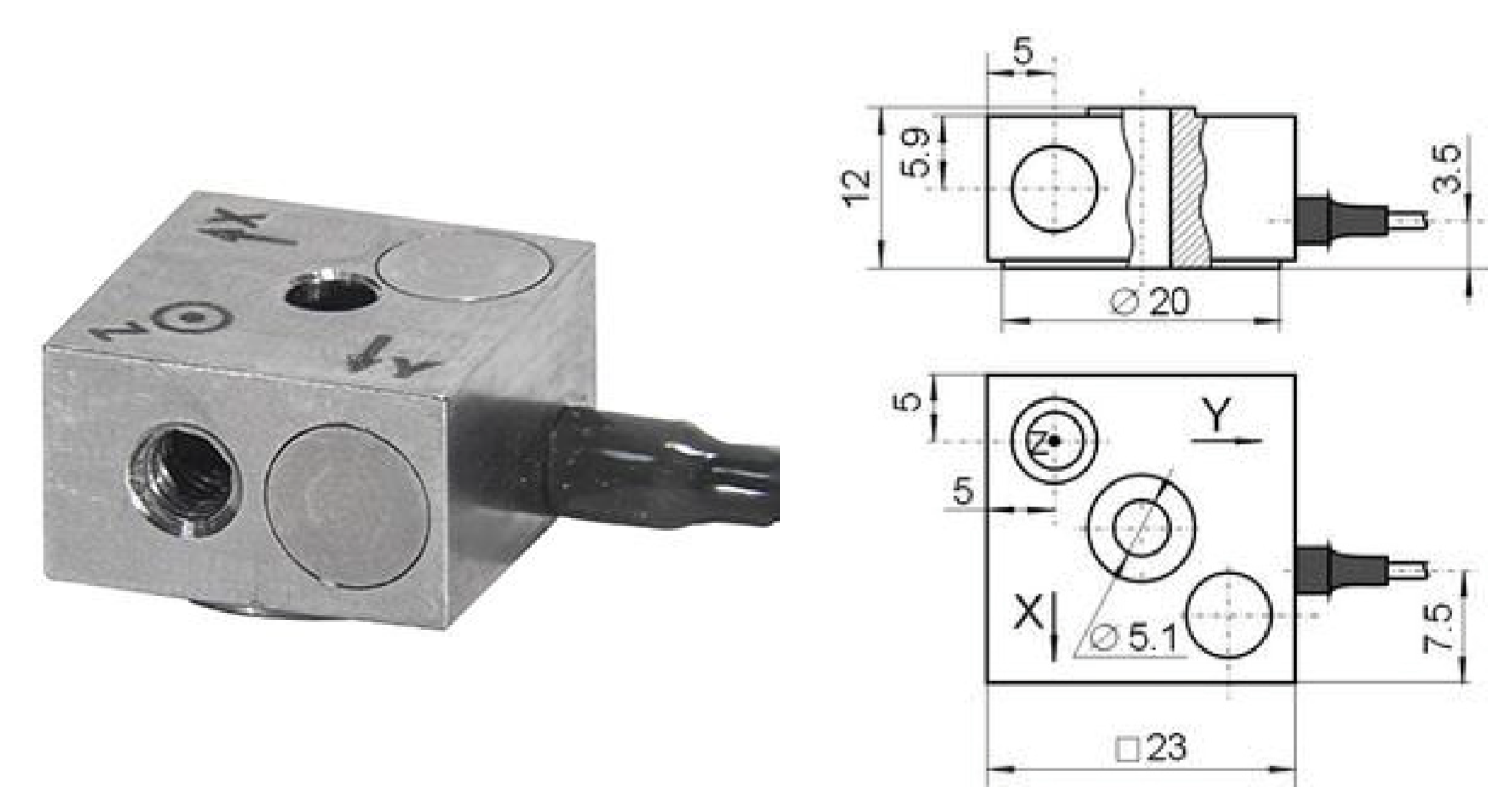
  7. Vibration Transducer AP2038P-100. Available online: https://globaltest.ru/product/vibropreobrazovatel-ap2038p-100/ (accessed on 20 January 2020).
  8. Saifullin, E.R.; Zagretdinov, A.R.; Ziganshin, S.G.; Vankov, Y.V. Control of the rotary equipment disbalance by the spectrum of envelope vibroacoustic signal. JARDCS 2018, 10, 2242–2247. [Google Scholar]
  9. Ziganshin, S.G.; Izmailova, E.V.; Maryashev, A.V. Technique for search of pipeline leakage according to acoustic signals analysis. In Proceedings of the electronic edition of the International Conference on Industrial Engineering, Applications and Manufacturing (ICIEAM 2017), St. Petersburg, Russia, 16–19 May 2017; IEEE: Piscataway, NJ, USA, 2017. [Google Scholar] [CrossRef]
  10. Vankov, Y.V.; Ziganshin, S.G.; Izmailova, E.V.; Serov, V.V. Determination of the oscillation frequencies of corrosion defects finite element methods in order to develop methods of acoustic monitoring of pipelines. In Proceedings of the IOP Conference Series: Materials Science and Engineering, International Scientific and Technical Conference “Innovative Mechanical Engineering Technologies, Equipment and Materials-2014” (ISC IMETEM 2014), Kazan, Russia, 3–5 December 2014; IOP Publishing: Bristol, UK, 2015. [Google Scholar] [CrossRef]
  11. Saifullin, E.R.; Ziganshin, S.G.; Vankov, Y.V.; Zagretdinov, A.R. Assessment of technical condition of polyurethane foam thermal insulation pipelines of heating networks using neural network technologies. IJET 2018, 7, 241–244. [Google Scholar] [CrossRef] [Green Version]
  12. Saifullin, E.R.; Ziganshin, S.G.; Vankov, Y.V.; Serov, V.V. Neural network analysis of vibration signals in the diagnostics of pipelines. J. Fundament. Appl. Sci. 2017, 9, 1139–1151. [Google Scholar] [CrossRef]
  13. LeCun, Y.; Bengio, Y.; Hinton, G.E. Deep Learning. Nature 2015, 521, 436–444. [Google Scholar] [CrossRef] [PubMed]
  14. Srivastava, R.K.; Greff, K.; Schmidhuber, J. Training very deep networks. In Proceedings of the 29th Annual Conference on Neural Information Processing Systems, Montreal, Canada, 7–12 December 2015; pp. 2377–2385. [Google Scholar]
  15. LeCun, Y.; Kavukcuoglu, K.; Farabet, C. Convolutional networks and applications in vision. In Proceedings of the 2010 IEEE International Symposium, Circuits and Systems (ISCAS), Paris, France, 30 May–2 June 2010; Volume 201, pp. 253–256. [Google Scholar]
  16. Jarrett, K.; Kavukcuoglu, K.; Ranzato, M.A.; LeCun, Y. What is the best multi-stage architecture for object recognition? In Proceedings of the International Conference on Computer Vision, Kyoto, Japan, 29 September–2 October 2009; pp. 2146–2153. [Google Scholar]
  17. Qian, P.; Tian, X.; Kanfoud, J.; Lee, J.L.Y.; Gan, T.-H. A Novel Condition Monitoring Method of Wind Turbines Based on Long Short-Term Memory Neural Network. Energies 2019, 12, 3411. [Google Scholar] [CrossRef] [Green Version]
  18. Chen, J.; Hu, W.; Cao, D.; Zhang, B.; Huang, Q.; Chen, Z.; Blaabjerg, F. An Imbalance Fault Detection Algorithm for Variable-Speed Wind Turbines: A Deep Learning Approach. Energies 2019, 12, 2764. [Google Scholar] [CrossRef] [Green Version]
  19. Gao, F.; Wu, X.; Liu, Q.; Liu, J.; Yang, X. Fault Simulation and Online Diagnosis of Blade Damage of Large-Scale Wind Turbines. Energies 2019, 12, 522. [Google Scholar] [CrossRef] [Green Version]
  20. He, K.; Zhang, X.; Ren, S.; Sun, J. Deep Residual Learning for Image Recognition. In Proceedings of the IEEE Conference on Computer Vision and Pattern Recognition (CVPR), Las Vegas, NV, USA, 27–30 June 2016; pp. 770–778. [Google Scholar]
  21. Szegedy, C.; Ioffe, S.; Vanhoucke, V. Inception-v4, Inception-ResNet and the Impact of Residual Connections on Learning. In Proceedings of the Thirty-First AAAI Conference on Artificial Intelligence, San Francisco, CA, USA, 4–9 February 2017; pp. 4278–4284. [Google Scholar]
  22. Szegedy, C.; Liu, W.; Jia, Y.; Sermanet, P.; Reed, S.; Anguelov, D.; Erhan, D.; Vanhoucke, D.; Rabinovich, A. Going deeper with convolutions. In Proceedings of the 2015 IEEE Conference on Computer Vision and Pattern Recognition (CVPR), Boston, MA, USA, 7–12 June 2015; pp. 1–9. [Google Scholar] [CrossRef] [Green Version]
  23. Krizhevsky, A.; Sutskever, I.; Hinton, G. ImageNet classification with deep convolutional neural networks. Adv. Neural Inf. Process. Syst. 2012, 25, 1097–1105. [Google Scholar] [CrossRef]
  24. Sutskever, I.; Martens, J.; Dahl, G.; Hinton, G. On the Importance of Momentum and Initialization in Deep Learning. In Proceedings of the 30th International Conference on Machine Learning, Atlanta, GA, USA, 16–21 June 2013; Volume 28, pp. 1139–1147. [Google Scholar]
  25. Ioffe, S.; Szegedy, C. Batch normalization: Accelerating deep network training by reducing internal covariate shift. In Proceedings of the 32nd International Conference on Machine Learning, Lille, France, 6–11 July 2015; Volume 37, pp. 448–456. [Google Scholar]
  26. Pinto, N.; Cox, D.D.; DiCarlo, J.J. Why is real-world visual object recognition hard? PLoS Comp. Biol. 2008, 4, 27. [Google Scholar] [CrossRef] [PubMed]
  27. Serre, T.; Wolf, L.; Poggio, T. Object recognition with features inspired by visual cortex. In Proceedings of the 2005 IEEE Computer Society Conference on Computer Vision and Pattern Recognition (CVPR’05), San Diego, CA, USA, 20–25 June 2005; pp. 994–1000. [Google Scholar]
  28. Duchi, J.; Hazan, E.; Singer, Y. Adaptive subgradient methods for online learning and stochastic optimization. J. Mach. Learn. Res. 2011, 12, 2121–2159. [Google Scholar]
  29. Lee, C.Y.; Gallagher, P.W.; Tu, Z. Generalizing pooling functions in convolutional neural networks: Mixed, gated, and tree. In Proceedings of the 18th International Conference on Artificial Intelligence and Statistics, Cadiz, Spain, 9–11 May 2016; pp. 464–472. [Google Scholar]
  30. Minyazev, R.S.; Rumyantsev, A.A.; Dyganov, S.A.; Baev, A.A. X-ray Image Analysis for the Neural Network-Based Detection of Pathology. Bull. Russ. Acad. Sci. Phys. 2018, 82, 1529–1531. [Google Scholar] [CrossRef]
  31. Nellore, S.B. Various performance measures in Binary classification—An Overview of ROC study. Int. J. Innov. Sci. Eng. Technol. 2015, 2, 596–605. [Google Scholar]
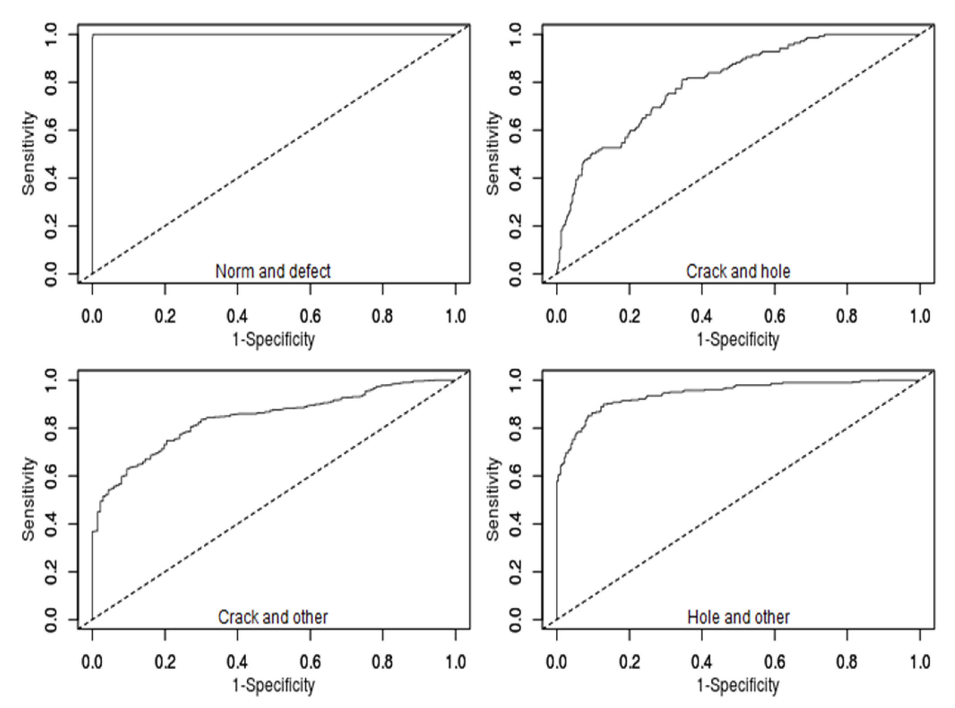
Figure 1. Experimental stand: (1) valve; (2) pressure gauge; (3) pipeline; (4) defect; (5) piezoelectric transducer; (6) check valve; (7) capacity; (8) pump; (9) ADC-DAC; (10) computer.
Energies 13 00618 g001
Figure 2. Pipeline defect model and method for fixing it.
Energies 13 00618 g002
Figure 3. Appearance and dimensions of the vibration transducer AP2038P.
Energies 13 00618 g003
Figure 4. Oscillation spectra of a defect-free pipeline: (a) signal along the X-axis at a pressure of 4 atm; (b) signal along the Y-axis at a pressure of 4 atm; (c) signal along the X-axis at a pressure of 3 atm; (d) signal along the Y-axis at a pressure of 3 atm; (e) signal along the X-axis at a pressure of 2 atm; (f) signal along the Y-axis at a pressure of 2 atm.
Energies 13 00618 g004
Figure 5. Frequency spectra of pipelines with defects (at a pressure of 3 atm): (a) signal on the X-axis of defect-free tubing; (b) signal along the Y-axis of defect-free tubing; (c) signal on the X-axis of the pipeline with a hole diameter of 1 mm; (d) signal on the Y-axis of the pipeline with a hole diameter of 1 mm; (e) signal on the X-axis of the pipeline with a hole diameter of 3 mm; (f) signal on the Y-axis of the pipeline with a hole diameter of 3 mm; (g) signal on the X-axis of the pipeline with the defect type “crack”; (h) signal on the Y-axis of the pipeline with the defect type “crack”.
Energies 13 00618 g005aEnergies 13 00618 g005b
Figure 6. (a) Detailed diagram of the algorithm for converting measurements to RGB images. (b) An example of processing acoustic signals: on the left, from a defect-free pipeline; in the center, from a pipeline with a defect of the “crack” type; on the right, from a pipeline with a defect of the “hole” type.
Energies 13 00618 g006
Figure 7. Block diagram of acoustic signal conversion and neural network training.
Energies 13 00618 g007
Figure 8. Graphs of Receiver Operating Characteristic (ROC) curves.
Energies 13 00618 g008
Table 1. The effectiveness of the neural network in the search for defects.
Criterion“Norm” and “Defect”“Crack” and “Hole”“Crack” and “Others”“Hole” and “Others”
TP (Sensitivity)0.9930.8100.7960.861
FP0.0250.3450.2530.097
TN (Specificity)0.9750.6550.7470.903
FN0.0070.1900.2040.139
PPV0.9030.3870.3950.899
NPV0.9980.9280.9460.865
PLR40.1680.4263.1448.830
NLR0.0073.4510.2740.154
AUC (Area Under the Curve)0.9990.8020.8390.943

