Planned Heating Control Strategy and Thermodynamic Modeling of a Natural Gas Thermal Desorption System for Contaminated Soil

Abstract

This paper presents a planned heating control strategy applied for a natural gas thermal desorption system for polluted soil to achieve the dynamic adjustment of the heating time and energy consumption. A lumped-parameter model for the proposed system is established to examine effects of the natural gas mass flow rate and the excess air coefficient on the heating performance of the target soil. The control strategy is explored to accomplish the heating process as expected with constant temperature change rate or constant volumetric water content change rate at different phases by adapting the natural gas flow. The results demonstrate that the heating plan can be realized within the scheduled 36 days and the total natural gas consumption can be reduced by 24% (1487 kg) compared to that of the open-loop reference condition, which may be widely applied for other thermal remediation systems of the polluted soil.

1. Introduction

Over the past few decades, soil contamination has become an increasingly prominent concern owing to accelerated industrialization and urbanization in China and all over the world [1,2,3]. This phenomenon is particularly severe in the vicinity of heavy industrial areas such as the coking plants, chemical plants and steelworks [4,5]. Among all kinds of hazardous substances released by industrial activities, heavy metals make a significant contribution to soil pollution [6] which are covert, persistent and irreversible [7]. Unlike organic pollutants, which may degrade to less harmful components by means of biological or chemical approaches, heavy metals are not degradable by natural processes. What is worse, this kind of pollution can easily enter into the food chain and also seriously threatens the health and well-being of animals and human beings [8,9]. Due to the severe damage of soil pollution and the severity of the situation, it is urgent that appropriate technologies of contaminated soil treatment are developed.

In situ thermal desorption (ISTD) is one of the remediation technologies for polluted soil and has attracted great research interest in recent years. This method uses fluid injection or heating elements to heat the contaminated site at sufficient temperature without excavation. As a result, most pollutants are separated from soil and collected by the aboveground off-gas treatment units for standardized discharge [10]. Compared with ex situ thermal desorption (ESTD), ISTD has advantages of suitability to various types of pollutants, a short remediation period, high efficiency and no secondary pollution [11,12,13]. For all this, it has been applied at a great many contaminated sites via different heating modes such as steam-enhanced extraction (SEE), electrical resistance heating (ERH) and thermal conduction heating (TCH). Heron et al. [14] introduced a combination remediation of SEE and ERH for a non-aqueous phase liquid (NAPL) site, where SEE was used to deliver energy to the permeable zones and ERH to heat low-permeable zones. By the removal of about 1130 kg of volatile contaminants within 4.5 months, soil and ground water concentrations were reduced to concentrations believed to be at least 100 times lower than standard levels.

In addition to various heating types, there are many other factors influencing the performance of the thermal desorption (TD) system, for instance, heating temperature, heating rate, physical and chemical properties of soil, initial concentration of contaminants, and so on [15,16,17,18]. Bulmau et al. [19] studied the effect of heating temperature on soils polluted by polycyclic aromatic hydrocarbons (PAHs) and indicated that the removal efficiency increased from 5% at 350 °C to 80% at 650 °C when processed for the same time. Qi et al. [20] found that the removal efficiencies after heating at 600 °C for 20 min, 40 min and 60 min are 20.86%, 64.47% and 95.7% respectively. The removal rate for polychlorinated biphenyls (PCBs) within the 20–40 min interval is greater than that of the first 20 min. Falciglia et al. [21] used TD to restore diesel-contaminated soils with particle sizes of 75–200 μm, 200–350 μm and 500–840 μm. The results showed that the removal efficiency of small particles is higher than that of large particles under the same heating condition. Zhang et al. [22] confirmed that with the same heating temperature and the same heating time, the removal efficiency rised as the initial concentration of nitrobenzene increased.

TCH is an effective soil-remediation technology in which the processes of heating and vacuum extraction are carried out simultaneously, either with heater blankets for surface and near-surface soil pollution or with an array of vertical heating wells for deep soil pollution [10]. Generally, the heating wells operate at 800 °C to 900 °C, near which radiation and conductive heat transfer dominate. In contrast, for the soil with greater distance from the heating well, heat conduction is the primary form of heating. When the soil is warmed to a high target temperature, the contaminants in the soil will vaporize and be drawn by the vacuum into the extraction wells with the assistance of the vacuum blower for aboveground treatment. Many studies have shown that with high temperature and long heating time, the pollutants in the heated soil are almost completely removed, with an extremely high removal efficiency [23,24].

Electricity is an energy source for TCH which is applied to most applications to date. Heron et al. [25] used TCH for treatment of a brownfields contaminated site near San Francisco, California. In this case, the target soil with a volume of 5097 m³ to a depth of 6.2 m was heated for a period of 110 days. A total of 2.2 million kWh of electric power was used to heat the site. Approximately 45% of this energy was used to heat the soil to the target temperature, and another 53% was used to boil about 41% of the groundwater within the treatment site. Chang et al. [26] presented an in situ thermal remediation experiment to clean up a mercury-polluted site in Taipei. The results showed that the primary factors affecting the thermal desorption treatment of mercury in soil were the temperature and the heating time. A site having eight chlorinated volatile organic compound source zones with a volume of 38,200 m³ was remediated through TCH and met the remedial objectives after 177 days [27]. Natural gas is another energy source for TCH named as gas thermal desorption (GTD). Compared to electric heating, natural gas heating has advantages of convenient for transfer, high power per unit heating length, large heating depth, equipment operation flexibility, and so on. Although many companies in different countries have been committed to the soil treatment using GTD and achieved great restore effect [28], there are few studies focused on the reduction of natural gas consumption with appropriate control strategy.

At present, the experimental research on the thermal remediation of soil pollution can be usually divided into two categories, namely, field experiments and laboratory experiments. The former [26,29] are conducted at an on-site contaminated area, while the latter [30] are carried out in the laboratory scale apparatus with a small portion of the soil excavated. For field experiments, it is extremely difficult to monitor the moisture transfer process within the heated soil as well as between the heated soil and the surrounding soil along the treatment duration using existing technologies. For laboratory experiments, likewise, owing to that the target recovery soil is excavated and put into a laboratory appliance individually, the moisture transfer between the heated site and the surrounding site during the heating process cannot be simulated veritably and accurately. Due to the disadvantages of the aforementioned experimental research, a lumped-parameter method is employed in the present study in order to investigate the influence of moisture migration on the heating performance of the soil. Furthermore, other correlative studies [31,32,33] by our team using a numerical simulation method or a lumped-parameter method have been conducted and published online.

In this paper, a planned heating control strategy of a natural gas thermal desorption system (GTDS) is proposed aiming to effectively heat the contaminated soil within the specified heating time with less energy consumption. Dynamic heat-transfer modeling for the GTDS on the basis of the lumped-parameter method is established. Simulation analyses are conducted to investigate the impacts of the natural gas mass flow rate and the excess air coefficient on the heating characteristics of the soil. A scheduled heating control strategy based on a group of proportional-integral-derivative (PID) controllers is designed to manipulate the temperature change rate or volumetric water content change rate of the soil by adjusting the natural gas mass flow rate, and the remediation time ultimately. Confronting various disturbances in excess air coefficient and external rainfall, the GTDS under this innovative control strategy can attain target heating temperature in terms of the evidently decreased natural gas consumption and the scheduled operational period with excellent control ability. The results proved that the carefully designed GTDS may have a broad prospect of application for contaminated soil remediation.

2. System Description and Dynamic Model

2.1. General Conception of Gas Thermal Desorption System (GTDS)

The schematic diagram of the GTDS for soil pollution is illustrated in Figure 1. It consists of the heating unit, extraction unit, ground insulation unit and off-gas treatment unit. The heating unit includes a burner fixed on the top of the well, a thermal well inserted vertically into the soil and a combustion blower placed aboveground at the outlet of the well. The natural gas and air are inhaled by the combustion blower into the combustor and burn along with the high temperature flue gas generated. The hot flue gas is injected downward into the inner pipe of the thermal well and then enters the annular space between the inner pipe and outer pipe then, finally, flows upward along the outer pipe and away from the outlet of the outer pipe. During the flow process of flue gas in the thermal well, heat is transferred to the restoration soil which is in contact with the outer pipe of thermal well. Provided there is high temperature for a long period, the volatile contaminants in the soil can vaporize and then be drawn by the extraction blower into the extraction well. This gaseous product is transported to the off-gas treatment unit to be purified for standardized discharge. Additionally, an insulating layer consisting of cellular concrete, insulating brick and rubble with certain thickness individually is laid on the surface of the soil in order to reduce heat loss and prevent pollutant diffusion during operation. Detailed geometric characteristics of the GTDS are provided in

Table A1. Geometric parameters of the GTDS.

Parameters		Value (mm)
Burner [35]	Inner diameter	200
	Outer diameter	210
	Length	1000
Thermal well [25]	Inner diameter of inner pipe	760
	Thickness of inner pipe	5
	Length of inner pipe	4700
	Inner diameter of outer pipe	1400
	Thickness of outer pipe	5
	Length of outer pipe	5000
Soil	Inner diameter	1410
	Outer diameter	4000
	Depth	5500

in Appendix A.

A large number of experimental research works [23,34] have revealed that during the remediation process, the temperature of the heated soil goes through three phases, namely, heat-up phase, boiling phase and superheating phase, which is depicted in Figure 2.

In the heat-up phase, the soil, consisting of solid particles as well as liquid water and vaporous water in the pores, is heated from initial temperature t_s0 to water’s boiling point t_s1. There exist inappreciable evaporation of liquid water and moisture migration from unheated sites in this stage. In the boiling phase, liquid water evaporates along with a constant temperature of the soil. At this point, all the heat generated from the thermal well is used to vaporize liquid water. With evaporation of liquid water in the heated soil, the amount of moisture migration from unheated sites increases gradually. When all the liquid water has been vaporized, the target soil enters into the next phase. In the superheating phase, the dry soil can be heated to the final target temperature, meanwhile, the fluid water permeated from unheated zones will evaporate immediately on account of the extremely high temperature. Furthermore, the contaminations can vaporize with the assistant of high temperature for further treatment.

Note that in the reminder of this paper, the three phases of heat-up phase, boiling phase and superheating phase are defined as Phase-1, Phase-2 and Phase-3 separately for the sake of simplicity.

Considering that in the actual construction, the operational period of remediation is generally uncontrollable beforehand but is extremely important not only for the remediation effect but also for the construction progress. To address this problem, a planned heating control strategy based on a group of PID controllers for the GTDS is put forward, as shown in Figure 3. As stated above in Figure 2, the volumetric water content (VWC) in Phase-1 varies little, the temperature during Phase-2 is constant at t_s1, and the VWC at Phase-3 is fixed to 0. Taking this into account, temperature variation rate of Phase-1, VWC change rate of Phase-2 and temperature rise rate of Phase-3 are selected as the target variables, moreover, mass flow rate of natural gas is set as the control variable.

Overall, the proposed control strategy comprised a planning layer and a control layer. The fundamental control concept is that by adjusting the natural gas flow, the target soil can be heated with constant temperature rise rate or constant VWC change rate in different stages and attain the objective temperature finally within the scheduled days. To be more specific, the overall heating period and the individual heating time of each phase are firstly determined according to the construction plan. According to both the heating time of each stage and the variation of each objective variable, the theoretical value is further calculated. The calculated value and actual value of each objective variable at different stages are respectively regarded as two inputs of the corresponding PID controllers. Based on the errors of the objective variables, the natural gas can be manipulated with corresponding mass flow rate and transported to the burner as the energy source of the GTDS.

2.2. Mathematical Modeling

In this section, the working principle of the GTDS is provided in terms of the mathematics and thermodynamics including the lumped-parameter model and the control model, which may contribute to a better understanding of the function and dynamic characteristics of the system.

2.2.1. Lumped-Parameter Model

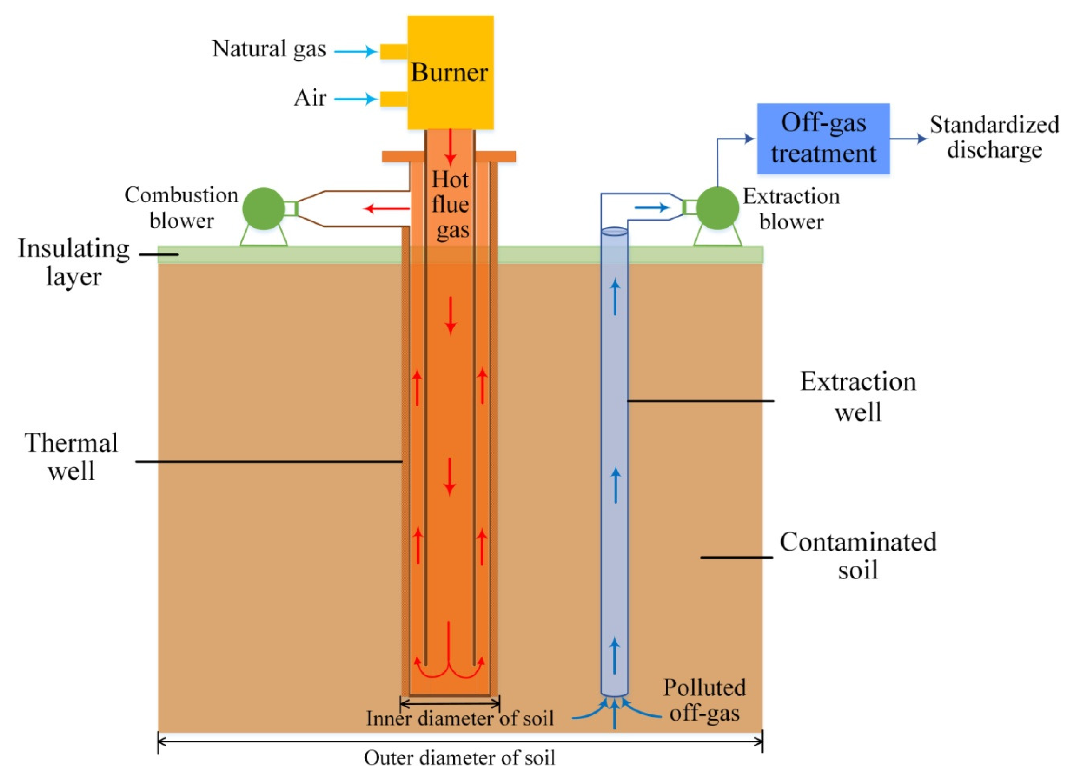
As illustrated in Figure 4a, a dynamic heat-transfer model based on the lumped-parameter method for the GTDS is proposed to investigate the thermal performance of the system in detail. In accordance with layout of the GTDS in Figure 1, the burner, the inner pipe of the heat well, the outer pipe of the heat well and the heated soil can be treated as four lumped-parameter nodes respectively, which will be fully described afterwards in this section.

1. Model of Burner

The schematic diagram of the burner is depicted in Figure 4b. Based on the energy conservation principle, the temperature dynamics of the burner can be expressed by [35,36]:

$$\left(m_b{c}_b\right)\stackrel{•}{t_b}=G_g{h}_g+G_a{h}_a+L_g{Q}_L-\frac{1}{R_b}\left(t_b-t_0\right)-G_f{h}_f,$$

(1)

where m_b is the mass of the burner; t_b and t₀ are the temperature of the burner and the ambient temperature; G_g, G_a and G_f are the mass flow rates of the natural gas, the air and the flue gas respectively; L_g is the volume flow rate of the natural gas; Q_L is low heating value of the natural gas; R_b is thermal resistance between the burner wall and burner crick; h_g, h_a and h_f are the enthalpies of the natural gas, the air and the flue gas which can be written as:

$$\{\begin{array}{l}{h}_g=c_g{t}_g\\ h_a=c_a{t}_a\\ h_f=c_f{t}_f\end{array},$$

(2)

where t_b, t_g and t_a are the temperatures of the burner, the natural gas and the air respectively; c_g, c_a and c_f are the specific heat of the natural gas, the air and the high temperature flue gas respectively. Thereby, c_f can be calculated by:

$$c_f={\displaystyle \sum g_i}{c}_{fi},$$

(3)

where g_i is mass fraction of the flue gas, c_fi is mass specific heat of components of the flue gas; the output flue gas temperature from the burner t_f can be expressed by:

$$t_f=t_0+{\eta }_b\left(t_b-t_0\right),$$

(4)

where η_b is the heat exchange efficiency of the burner.

In addition, G_a and G_f are given by Equations (5) and (6) respectively, where V₀ is theoretical volume of the air for complete combustion of the natural gas, $\alpha$ is excess air coefficient.

$$G_a=\frac{G_g}{{\rho }_g}\cdot V_0\cdot \alpha \cdot {\rho }_a;$$

(5)

$$G_f=G_g+G_a.$$

(6)

2. Model of Thermal Well

Figure 4c illustrates individual temperature points of the heat well. The temperature dynamics of the inner pipe and outer pipe of the thermal well, which are based on the energy conservation principle, are represented by Equations (7)–(8) [31,37]:

$$\left(m_{W1}{c}_{W1}\right)\stackrel{•}{t_{W1}}=G_f{c}_f{\eta }_W\left(t_{fi1}-t_{W1}\right)-{\epsilon }_a{A}_1{C}_0\left[{\left(\frac{T_{W1}}{100}\right)}^4-{\left(\frac{T_{W2}}{100}\right)}^4\right],$$

(7)

$$\left(m_{W2}{c}_{W2}\right)\stackrel{•}{t_{W2}}=G_f{c}_f{\eta }_W\left(t_{fi2}-t_{W2}\right)+{\epsilon }_a{A}_1{C}_0\left[{\left(\frac{T_{W1}}{100}\right)}^4-{\left(\frac{T_{W2}}{100}\right)}^4\right]-\frac{1}{R_{Ws}}\left(t_{W2}-t_s\right),$$

(8)

where m_W1 and m_W2 are the mass of the inner pipe and outer pipe; t_W1, t_W2 and t_s are the temperatures in Celsius of the inner pipe, the outer pipe and the heated soil respectively; T_W1 and T_W2 are Kelvin temperatures of the inner pipe and outer pipe; t_fi1 and t_fi2 are the input temperatures of the flue gas that flows into the inner pipe and the outer pipe; c_W1 and c_W2 are the specific heat of the inner pipe and outer pipe; η_W is the heat-exchange efficiency of the thermal well; R_Ws is thermal resistance between the outer pipe and the soil; C₀ is the black-body radiation coefficient; A₁ and A₂ are surface area of the inner pipe and outer pipe; ε₁ and ε₂ are the emissivity of the inner pipe and outer pipe; ε_a is the system emissivity which is defined in Equation (9) [38].

$${\epsilon }_a=\frac{1}{\frac{1}{{\epsilon }_1}+\frac{A_1}{A_2}\left(\frac{1}{{\epsilon }_2}-1\right)}.$$

(9)

Equations (10) and (11) present the output flue gas temperatures from the inner pipe (t_fo1) and that from the outer pipe (t_fo2) respectively. As clearly depicted in Figure 4c, t_fo1 is actually the input flue gas temperature of the outer pipe (t_fi2), which is expressed by Equation (12).

$$t_{fo1}=t_{fi1}+{\eta }_W\left(t_{W1}-t_{fi1}\right);$$

(10)

$$t_{fo2}=t_{fi2}+{\eta }_W\left(t_{W2}-t_{fi2}\right);$$

(11)

$$t_{fi2}=t_{fo1}.$$

(12)

3. Model of Heated Soil

For simplicity, some assumptions are made as follows:

(1)

The soil is homogeneous porous medium and there is no chemical interaction in the soil.

(2)

Solid, liquid, and gas phases are separately continuous in unsaturated soil.

(3)

Natural convection of fluids in the soil satisfies Darcy’s law.

(4)

The target site is considered as one of the unit blocks and each block is heated by a thermal well individually. There is no heat exchange between the heated site and the surrounding sites at the boundary.

(5)

There is no moisture transfer between the target heated site and the surrounding heated sites, moreover, the moisture transfer mainly occurs between the heated soil and the underlying unheated soil.

(6)

The influence of gravity on the soil moisture transfer in the unsaturated soil is assumed to be negligible.

(7)

The pressure inside the soil is evenly distributed.

(8)

The gases in the soil are assumed to be ideal.

(a) Liquid flow model

Based on the mass conservation principle, the VWC variation Equation [39] can be written as:

$$\left({\rho }_w{V}_s\right)\stackrel{•}{{\theta }_s}=m_{wi}-m_{wv},$$

(13)

where θ_s is the VWC of the soil, ρ_w is density of liquid water, V_s is volume of the soil, m_wv represents mass of vaporized liquid water, and m_wi denotes mass of liquid water flowing vertically into the heated soil [40] which is given by:

$$m_{wi}=J_{wi}{A}_{cs},$$

(14)

where A_cs is the migration area of liquid water in the vertical direction, J_wi is the liquid water migration flux density.

A lot of research [41,42,43,44] has shown that water seepage in the unsaturated soil is primarily caused by the temperature gradient and the moisture gradient. The liquid water migration flux density J_wi can be expressed by Equation (15) in line with Assumptions (5)–(6),

$$\overrightarrow{J_{wi}}=-{\rho }_w{K}_w\left(\nabla {\psi }_t\right)=-{\rho }_w\left(D_{wt}\frac{\partial t_s}{\partial l}+D_{w\theta }\frac{\partial {\theta }_s}{\partial l}-K_w\right),$$

(15)

where t_s is temperature of the heated soil, D_wt and D_wθ are the mass diffusivities of the liquid water in soil caused by temperature gradient and moisture gradient respectively; l is the transfer distance of the liquid water in the vertical direction, K_w is the hydraulic conductivity of the soil [45,46] which is defined by:

$$K_w=K_{ws}\cdot {\left(\frac{{\theta }_s}{\epsilon }\right)}^{\left(2b+3\right)},$$

(16)

ε is the void ratio of the soil, K_ws is saturated hydraulic conductivity, b is the characteristic coefficient of the soil.

(b) Vapor flow model

Likewise, on the basis of mass conservation principle, the mass equation of vapor can be written as:

$${\rho }_v\stackrel{•}{V_{vs}}=m_{wv}-m_{vo},$$

(17)

where V_vs is vapor volume in the soil, ρ_v is density of vapor water, m_vo is mass of vapor water extracted into the extraction well which is defined by:

$$m_{vo}=\frac{N_e}{P_{eo}-P_v}\cdot \frac{P_v}{R_v{T}_v},$$

(18)

where N_e is the power of the extraction blower, P_eo is the outlet pressure of the extraction blower, R_v is the gas constant of vapor water, T_v is Kelvin temperature of the vapor water.

Based on Assumption (7), provided that the volume of vapor in the soil pores V_vs and that in the extraction well V_{v_e} are considered as a whole, the pressure variation equation can be derived from Equations (17) and (18) that:

$$\left(V_{v\_e}+V_{vs}\right)\stackrel{•}{P_v}=R_v{T}_v{m}_{wv}-\frac{N_e}{P_{eo}-P_v}\cdot P_v.$$

(19)

(c) Heat-Flow Model

As presented in Figure 5, the temperature dynamics of the soil [31,33] can be expressed by:

$$\left(m_s{c}_s\right)\stackrel{•}{t_s}=Q_W+Q_w-Q_{up}-Q_{down}-Q_{eva}-Q_v,$$

(20)

where Q_W is heating power of the thermal well; Q_up and Q_down are heat leakage between the heated site and the insulating layer, as well as that between the heated site and the underlying unheated soil; Q_W, Q_up and Q_down can be calculated by:

$$\{\begin{array}{l}{Q}_W=\frac{1}{R_{Ws}}\left(t_{W2}-t_s\right)\\ Q_{up}=\frac{1}{R_{su}}\left(t_s-t_u\right)\\ Q_{down}=\frac{1}{R_{sd}}\left(t_s-t_d\right)\end{array}.$$

(21)

Q_w and Q_v represent the heat flux of liquid water migration and vapor water extraction respectively which can be given by:

$$\{\begin{array}{l}{Q}_w=m_{wi}{h}_w\\ Q_v=m_{vo}{h}_v\end{array}$$

(22)

where h_w and h_v are specific enthalpy of liquid water and vaporous water, m_wi and m_vo can be calculated by Equations (14) and (18).

Q_eva indicates the energy absorbed by liquid water evaporation which is defined by:

$$Q_{eva}=m_{wv}H,$$

(23)

where H is latent heat of evaporation.

2.2.2. Fluid-Flow Model

As shown in Figure 6, the overall flow resistance network of the gaseous fluids for the GTDS is a non-linear parallel and series flow network which can be expressed in detail by the following equations. Specifically, the fluid flow network comprises of the inlet natural gas pipe and inlet air pipe which are connected in parallel, as well as the burner wall, the heat well inner pipe, the heat well outer pipe and the flue gas outlet pipe which are associated in series. When the gaseous fluids such as natural gas, air and flue gas flow through the above channels, there exist flow resistances correspondingly which can be expressed by Equation (24) [47], where μ is the fluid viscosity, l is the channel length, ξ is the equivalent coefficient of channel length considering the bend and corner [48].

$$R=\frac{128\mu l\left(1+\xi \right)}{\pi d^4}.$$

(24)

Given the flow resistance of the inlet natural gas pipe R_g and that of the inlet air pipe R_a calculated from Equation (24), the parallel flow resistance R_par [49,50] can be presented by Equation (25), where ϕ_g and ϕ_a characterize the valve opening of the inlet natural gas pipe and air pipe. After that, the overall flow resistance R_net is proposed in Equation (26) where R_b, R_wi, R_wo and R_po are the flow resistances corresponding to each series branches as expressed in Figure 6.

$$R_{par}={\left(\frac{{\phi }_g}{\sqrt{R_g}}+\frac{{\phi }_a}{\sqrt{R_a}}\right)}^{-2};$$

(25)

$$R_{net}=R_{par}+R_b+R_{wi}+R_{wo}+R_{po}.$$

(26)

For a given pressure difference ΔP_c defined in Equation (27), where P_ci and P_co denote the inlet pressure and outlet pressure of the combustion blower respectively, the mass flow rate of flue gas through the fluid loop G_f can be written as Equation (28).

$$\Delta P_c=P_{co}-P_{ci};$$

(27)

$$G_f=\sqrt{\Delta P_c/R_{net}}.$$

(28)

According to Equations (5) and (6), the natural gas mass flow rate G_g and the air mass flow rate G_a can be separately expressed by Equations (29) and (30), correspondingly. Furthermore, the natural gas inlet pressure P_g and the air inlet pressure P_a can be obtained by Equations (31) and (32), where P_b is inlet pressure of the burner.

$$G_g=G_f\cdot \frac{{\rho }_g}{{\rho }_g+V_0\alpha {\rho }_a};$$

(29)

$$G_a=G_f\cdot \frac{V_0\alpha {\rho }_a}{{\rho }_g+V_0\alpha {\rho }_a}.$$

(30)

$$P_g=G_g^2{R}_g+P_b;$$

(31)

$$P_a=G_a^2{R}_a+P_b.$$

(32)

2.2.3. Planned Heating Control Model

The block diagram of the GTDS with planned heating control is shown in Figure 7. On the basis of conventional PID control, the amount of the natural gas is adjusted according to the difference of temperature variation rate or VWC variation rate at different stages, and finally achieve the heating plan in a specific number of days with less energy consumption. Whatever phase the soil is heated to, the temperature variation and the VWC variation can be calculated by:

$$\{\begin{array}{l}{\nu }_{ts}=t_{s\left(n+1\right)}-t_{s(n)}\\ {\nu }_{\theta s}={\theta }_{s\left(n+1\right)}-{\theta }_{s(n)}\end{array},$$

(33)

where n is the step size.

As inputs of the three PID controllers, the control error e₁, e₂ and e₃ are described by:

$$\{\begin{array}{l}{e}_1={\nu }_{ts1}^{\prime }-{\nu }_{ts1}\\ e_2={\nu }_{\theta s2}^{\prime }-{\nu }_{\theta s2}\\ e_3={\nu }_{ts3}^{\prime }-{\nu }_{ts3}\end{array},$$

(34)

where ${\nu }_{ts1}^{\prime }$, ${\nu }_{\theta s2}^{\prime }$ and ${\nu }_{ts3}^{\prime }$ are desired temperature change rate in Phase-1, the wanted VWC change rate in Phase-2 and the desired temperature change rate in Phase-3 respectively; v_ts1, v_ts2 and v_ts3 are actual values correspondingly.

With the assistance of the merge module, the mass flow rate of the natural gas (G_g) which is the energy input of the burner can be given by Equation (35), where G_g1, G_g2, G_g3 are the mass flow rate of the natural gas at each stage respectively.

$$G_g=\{\begin{array}{ll}{G}_{g1}=K_{p1}{e}_1+K_{i1}{\displaystyle \int e_{1}d\tau }+K_{d1}\frac{d{e}_1}{d\tau }& \left(t_s<100\right)\\ G_{g2}=K_{p2}{e}_2+K_{i2}{\displaystyle \int e_{2}d\tau }+K_{d2}\frac{d{e}_2}{d\tau }& \left(t_s=100\right)\\ G_{g3}=K_{p3}{e}_3+K_{i3}{\displaystyle \int e_{3}d\tau }+K_{d3}\frac{d{e}_3}{d\tau }& \left(t_s>100\right)\end{array}.$$

(35)

2.2.4. Simulation Condition Settings

Related parameter determinations of the GTDS and the original state of the system are summarized in

Table A2. Parameter determinations of the GTDS.

Parameter (Unit)	Symbol	Value
Natural gas [35,51,52]
Density (kg/m3)	ρg	0.728
Specific heat (J∙kg−1∙K−1)	cg	2185
Low heating value (J/m3)	QL	34539
Inlet temperature (°C)	tg	20
Dynamic viscosity (μ∙Pa∙s)	μg	11.06
Inlet pressure (kPa)	Pg	103.325
Air [53]
Density (kg/m3)	ρa	1.29
Specific heat (J∙kg−1∙K−1)	ca	1000
Inlet temperature (°C)	ta	20
Dynamic viscosity (μ∙Pa∙s)	μa	18.37
Inlet pressure (kPa)	Pa	101.325
Burner [38,53]
Mass (kg)	mb	25.26
Specific heat (J∙kg−1∙K−1)	cb	472
Thermal resistance (K/W)	Rb	0.096
Heat exchange efficiency	ηb	0.7
Thermal well [38,53,54]
Mass (kg)	mw1	443
	mw2	865
Specific heat (J∙kg−1∙K−1)	cw	472
Emissivity	ε0	0.35
black-body radiation coefficient (W∙m−2∙K−4)	C0	5.67
Heat exchange efficiency	ηw	0.9
Dynamic viscosity (μ∙Pa∙s)	μf	15.05
Soil [39,40]
Density (kg/m3)	ρdry	1580
	ρw	1000
	ρv	0.6
Void ratio	ε	0.45
Initial VWC (m3∙m−3)	θs0	0.25
Inlet temperature (°C)	ts0	20
Latent heat of evaporation (J/kg)	H	2,257,200

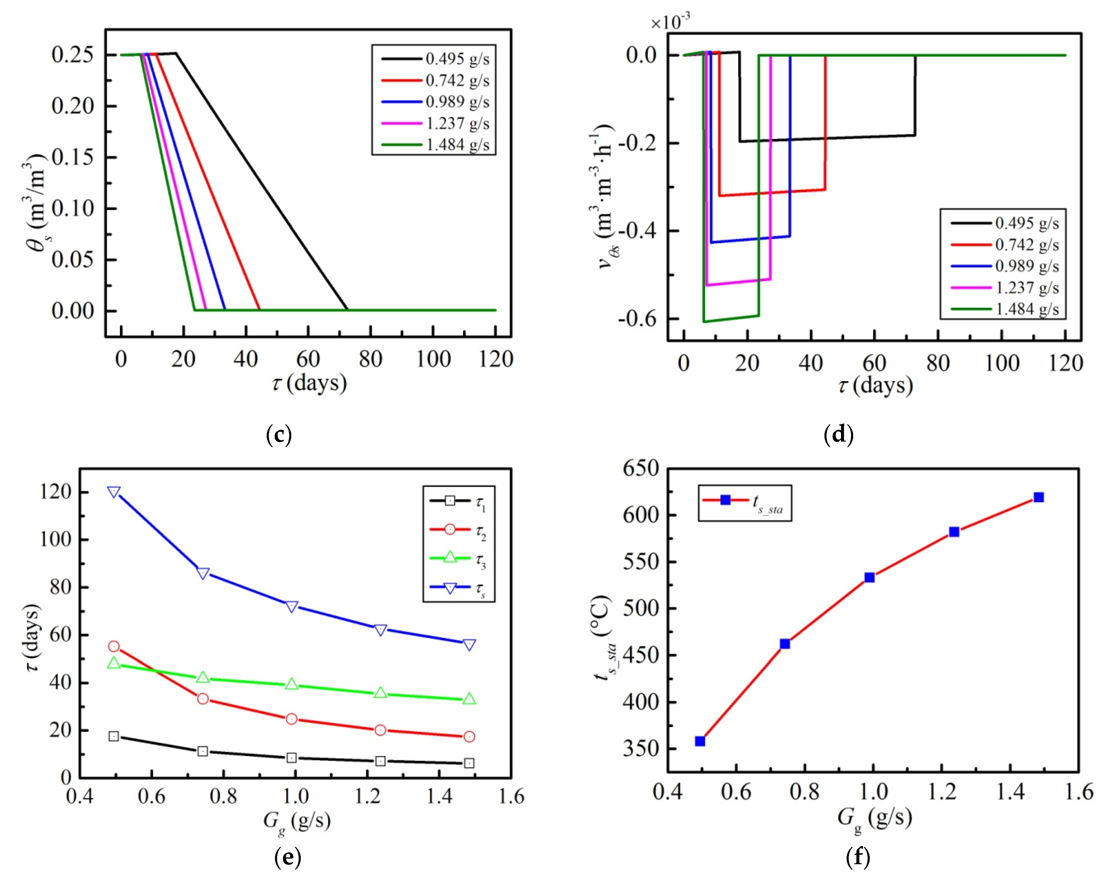
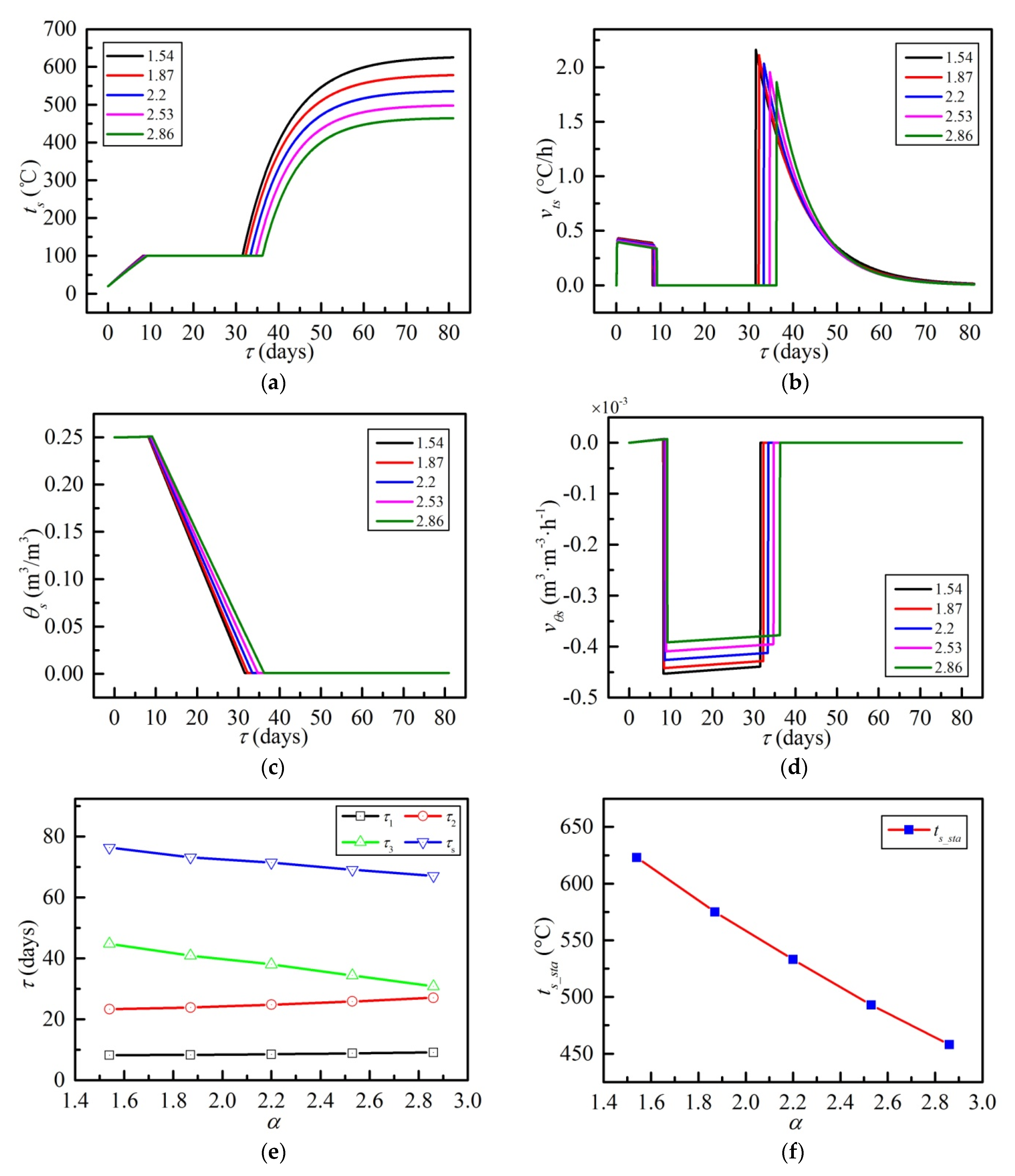
in Appendix B. The mass flow rate of the natural gas (G_g) and excess air coefficient (α) are two primary input variables which will be changed and controlled throughout the simulation process. As the base line for transient performance and control effect analyses, the initial G_g is 0.989 × 10⁻³ kg/s, and the initial α is 2.2.

Matlab R2017a was used as the simulation software. The flowchart of the simulation process is illustrated in Figure 8 which can be described in detail as follows: (1) the program is initialized at the beginning in accordance with the parameters tabulated in Table A2. (2) The simulation time and the calculation step are set. (3) Initial parameters are provided. (4) The desired values of ${\nu }_{ts1}^{\prime }$, ${\nu }_{\theta s2}^{\prime }$ and ${\nu }_{ts3}^{\prime }$ are derived. (5) The actual values of v_ts1, v_ts2 and v_ts3 can be obtained by Equations (1)–(23) and Equation (33). (6) During the closed-loop control, the control errors e₁, e₂ and e₃ can be calculated by Equation (34) firstly; and then G_g can be adjusted according to Equation (35). (7) After all the above procedures, two judgments need to be made. The first judgment is whether the control objective is convergence. If no, the simulation process will be updated by the new control parameters. If the first judgment is yes, the simulation continues to the second judgment, which is whether the simulation will continue. If the second judgment is yes, the simulation will jump to step (2). If the second judgment is no, the simulation will end.

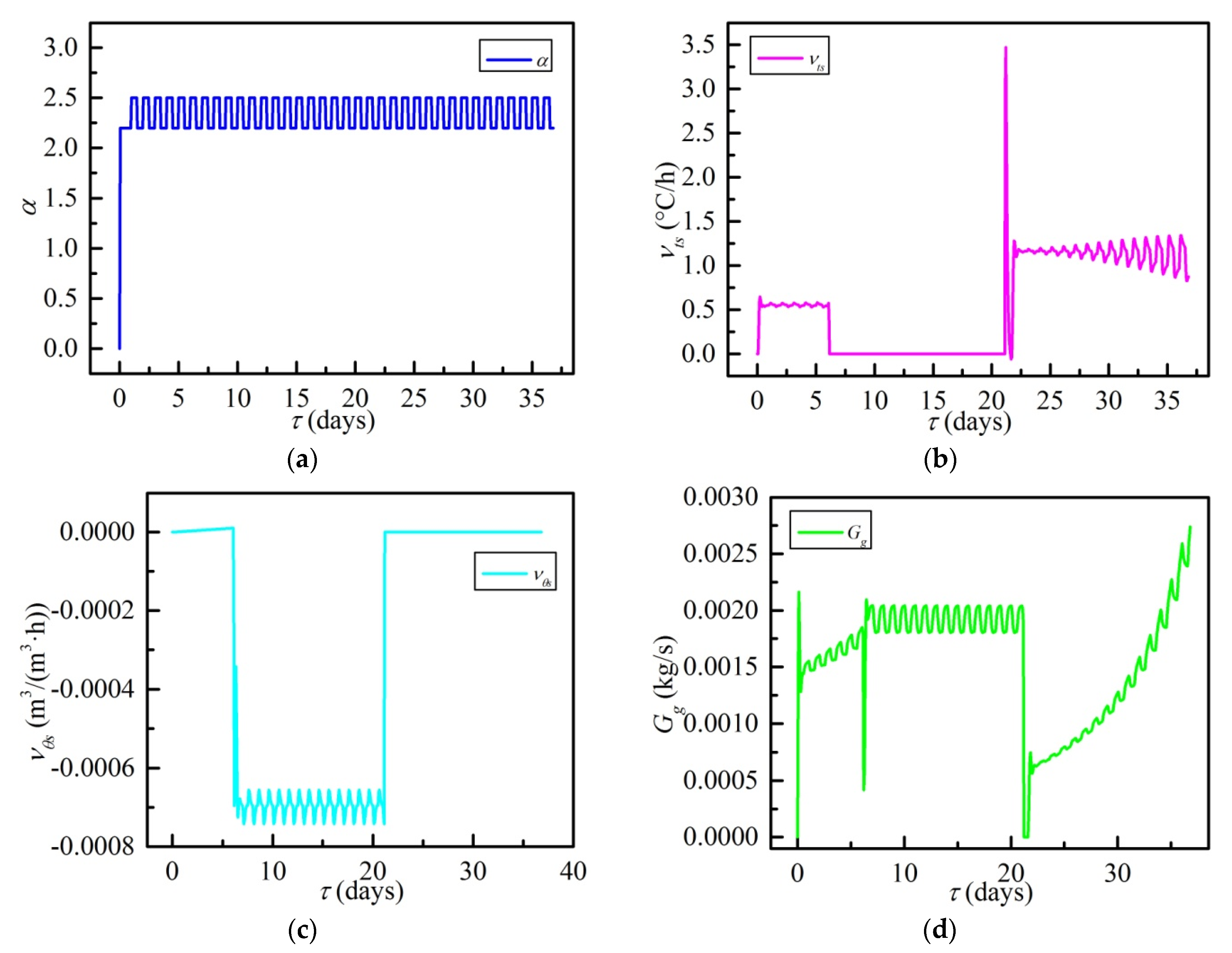
For investigating the effects of various input variables on the heating performance of the target soil, two simulation conditions are organized and listed in

Table 1. Case arrangement for open-loop dynamic analyses.

Simulation Conditions	Final Value	Description	Objective Variable
Natural gas mass flow rate variation	0.495 × 10−3 kg/s	50% step decrease	Temperature and VWC of the target soil
	0.742 × 10−3 kg/s	25% step decrease
	0.989 × 10−3 kg/s	Baseline value
	1.237 × 10−3 kg/s	25% step increase
	1.484 × 10−3 kg/s	50% step increase
Excess air coefficient variation	1.54	30% step decrease
	1.87	15% step decrease
	2.2	Baseline value
	2.53	15% step increase
	2.86	30% step increase

. Two simulation conditions are organized and listed in Table 1. To be specific, various step disturbances in the input G_g and α take place to demonstrate the influence of the natural gas mass flow rate and the excess air coefficient upon the soil’s heating characteristics.

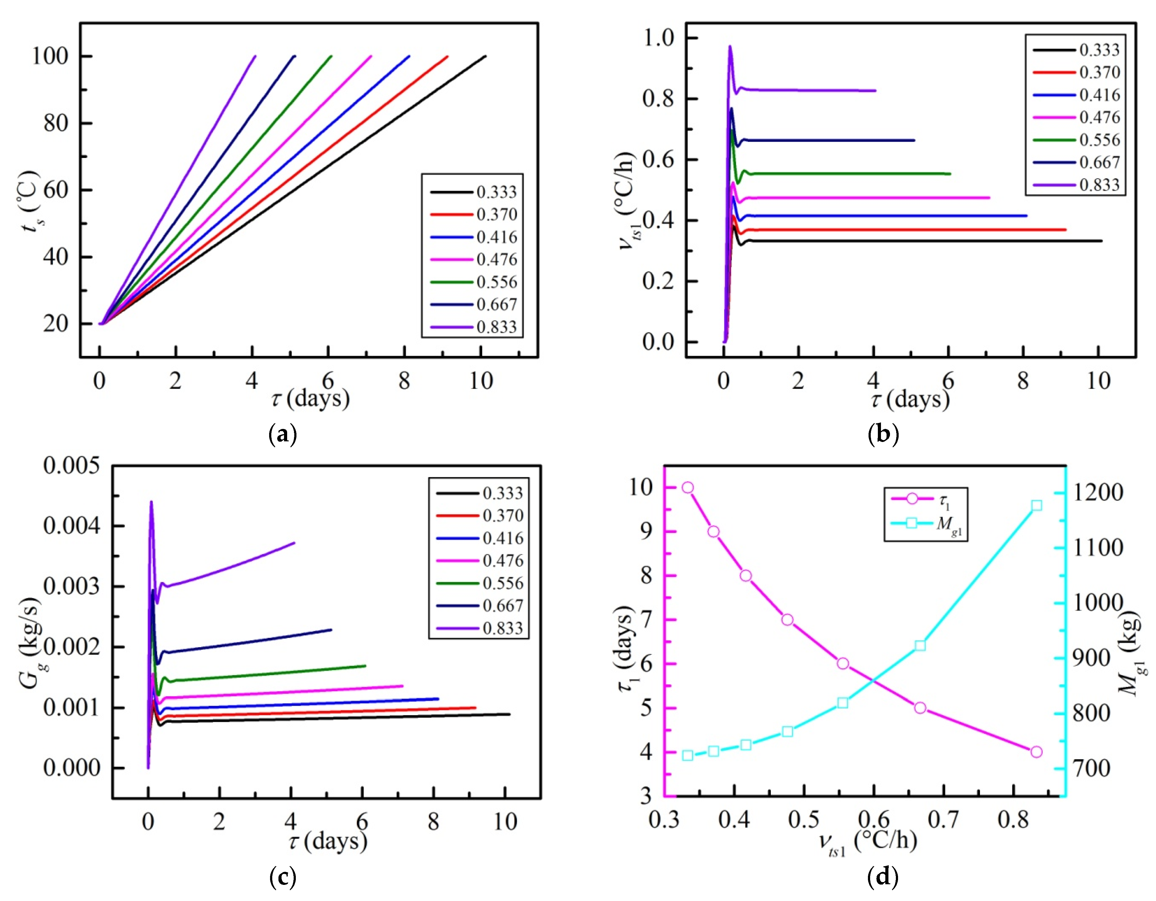
Given a fixed temperature variation or VWC variation, the desired temperature change rate (${\nu }_{ts}^{\prime }$) or desired VWC change rate (${\nu }_{\theta s}^{\prime }$) vary with the heating time at different phases. For the purpose of investigating the influence of ${\nu }_{ts}^{\prime }$ or ${\nu }_{\theta s}^{\prime }$ on the system performances, simulation conditions for each phase are offered in

Table 2. Simulation conditions for three phases.

Heating Phase	Heating Time (Days)	Variation Quantity	Change Rate
Phase-1	4	80 °C	0.8333 °C/h
	5		0.6667 °C h
	6		0.5556 °C/h
	7		0.4762 °C/h
	8		0.4167 °C/h
	9		0.3704 °C/h
	10		0.3333 °C/h
Phase-2	10	−0.2505 m3/m3	−0.0010439 m3/(m3·h)
	15		−0.0006965 m3/(m3·h)
	20		−0.0005219 m3/(m3·h)
	25		−0.0004175 m3/(m3·h)
	30		−0.000348 m3/(m3·h)
Phase-3	10	425 °C	1.77083 °C/h
	15		1.18056 °C/h
	20		0.88542 °C/h
	25		0.77083 °C/h
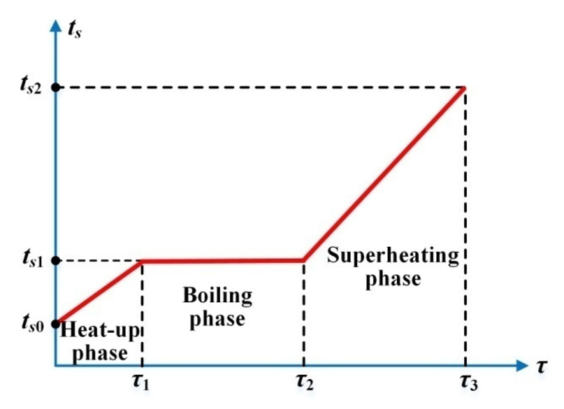
	30		0.59028 °C/h

. It is worth noting that the initial temperature and the objective temperature of soil are assumed to be 20 °C and 525 °C, respectively, which leads to the temperature change of Phase-1 being 80 °C and that of Phase-3 being 425 °C. Moreover, considering an original VWC of 0.25 m³/m³ and the VWC increment of 0.0005 m³/m³ in Phase-1, the VWC variation of Phase-2 is −0.2505 m³/m³. Determinations of relevant PID parameters are summarized in

Table 3. Parameters of the simulated proportional-integral-derivative (PID) controllers.

Controllers	Parameters
	Kp	Ki	Kd
PID-1	2.5 × 10−3	2.5 × 10−7	0
PID-2	2	3 × 10−4	0
PID-3	4 × 10−4	4 × 10−8	0

.

In addition, to investigate the performance in rejecting disturbances of the controller, two cases are arranged and listed in

Table 4. Case arrangement for closed-loop control effect analyses.

Simulation Conditions	Inputs	Description	Control Variable	Objective Variable
Periodic disturbance	α	Square wave periodic disturbance with high level of 2.5 and low level of 2.3	Mass flow rate of natural gas	Temperature change rate for Phase-1 and Phase-3, VWC change rate for Phase-2
Step disturbance	Gwi	100% step increase lasting for 4 days in each of the three phases

.

3. Open-Loop Dynamic Characteristics

The focus of this section is to investigate the effects of the natural gas mass flow rate G_g and excess air coefficient α on the temperature characteristic and moisture characteristic of the heated soil. Due to that the soil heating process is a slowly varying process, the sampling step is set as 3600 s (1 h) for simulation.

3.1. Disturbance of Natural Gas Mass Flow Rate

Figure 9 presents the temperature and VWC characteristics of the target soil under various step disturbances in G_g corresponding to the first simulation condition in Table 1. Note that the G_g of 0.989 × 10⁻³ kg/s is considered as a baseline working condition with other four conditions. In Figure 9a, take the baseline condition (0.989 × 10⁻³ kg/s) which is represented by the blue for instance, t_s rises from 20 °C to 100 °C within the first 8.5 days (Phase-1), and then is fixed at 100 °C in the next 24.8 days (Phase-2), in Phase-3, it goes up rapidly from 100 °C and settles at 532 °C ultimately in the last 39 days. For other cases, t_s presents the same trend as well. The variation trend of the soil temperature is highly consistent with the research results in related literatures [23,34].

The variation of t_s can be further elaborated by v_ts which is shown in Figure 9b. For the baseline case in Phase-1, v_ts decreases slowly within the range from 0.42 °C /h to 0.36 °C /h; in Phase-2, v_ts keeps 0 all the time; in Phase-3, v_ts raises sharply to the maximum of 2.03 °C /h firstly, then declines gradually and attains stabilization of nearly 0 °C/h ultimately. For other conditions, the overall trend is the same as the baseline condition.

Figure 9c provides the VWC (θ_s) variation under various G_g. When G_g is 0.989 × 10⁻³ kg/s, θ_s exhibits a slight increase from 0.25 m³/m³ to 0.2505 m³/m³ at Phase-1; in Phase-2, θ_s declines considerably from 0.2505 m³/m³ to 0 m³/m³ owing to the large evaporation amount of liquid water; during Phase-3, θ_s remains unchanged of 0 m³/m³. For further explaining, Figure 9d reflects the variation of v_θs under different G_g. In accordance with θ_w, v_θs is nearly 0 in Phase-1 and remains 0 during Phase-3, but presents a slow rise in Phase-2.

The individual heating time of three phases τ₁, τ₂ and τ₃ as well as the total heating period τ_s at different G_g are plotted in Figure 9e. With the increase in G_g, τ₁ decreases from 17.6 days to 6.25 days, τ₂ descends from 55.2 days to 17.3 days, τ₃ drops from 47.9 days to 32.8 days. In addition, the sum of τ₁, τ₂ and τ₃, τ_s keeps the downward tendency as well. The stable temperature of the soil (t_{s_sta}) at various G_g is depicted in Figure 9f. It can be viewed that t_{s_sta} raises exponentially from 358 °C to 619 °C with the increase in G_g from −50% step-disturbance to +50% step-disturbance.

The above observations demonstrate that the natural gas consumption has a decisive effect on the heating performance of the GTDS absolutely. As for the baseline condition (G_g = 0.989 × 10⁻³ kg/s), the heating period is 72.3 days and the natural gas consumption is 6182 kg. More natural gas applied to the GTDS leads to a higher stable temperature and a shorter remediation time of the target site. However, the higher the G_g, the more energy the system will consume, which is not preferable. Aiming to balance the energy consumption and the heating duration which are two dominating parameters in this paper, control strategy analyses in different stages will be conducted in Section 4.1.

3.2. Disturbance of Excess Air Coefficient

The characteristics of soil under different disturbances in α in line with the second simulation condition in Table 1 are expressed in Figure 10. Figure 10a,b present the variations of t_s and v_ts with various α. Taking the case of 1.87 for example, t_s increases with a slightly decreased v_ts from in Phase-1; and then both t_s and v_ts are unchanged all the while in Phase-2; finally, t_s rises rapidly with a sharply declined v_ts in Phase-3. The duration of three phases are 8.3 days, 23.9 days and 40.96 days, respectively.

The VWC (θ_s) variation and VWC change rate (v_θs) variation under different α are graphed in Figure 10c,d respectively. For all the five conditions, the overall variant trend of θ_s and v_θs are similar to that in Figure 9c,d in Section 3.1. Note that v_θs is nearly close to 0 and θ_s exhibits a slight increase in Phase-1; θ_s and v_θs remains 0 in Phase-3; whereas in Phase-2, θ_s goes down to 0 m³/m³ gradually and the corresponding v_θs shows a slow rise. Furthermore, for the second phase, the greater the α is, the smaller the absolute value of v_θs, and the longer it takes for θ_s to decline to 0 m³/m³.

As revealed in Figure 10e, when confronting disturbances in α ranging from 1.54 to 2.86, τ₁ presents a slight rise from 8.2 days to 9.3 days, τ₂ exhibits an obvious increase from 23.3 days to 27 days, whereas, τ₃ decreases considerably from 44.8 days to 30.8 days. The combination of τ₁, τ₁ and τ₃ yields that τ_s declines by 9.3 days accordingly. Figure 10f reflects that t_{s_sta} decreases linearly at a rate of −125 approximately with the increase in α.

The analyses stated above suggest that the excess air coefficient exerts a significant influence upon the soil’s temperature and VWC characteristics. Provided that the mass flow rate of natural gas is constant and the excess air coefficient is greater than 1.05, less air brought to the burner results in a higher stable temperature and a shorter heating period. This can be explained by the fact that proper increase of excess air coefficient can reduce the heat loss of chemical incomplete combustion; too high an excess air coefficient, however, will reduce the furnace temperature and yield incomplete combustion.

4. Closed-Loop Control Effect Analyses

In this section, the GTDS with the well-designed planned heating controller is firstly discussed in terms of various temperature change rates or VWC change rates in different phases, and then responses to disturbances in the excess air coefficient and liquid water migration quantity for closed-loop simulation, which is based on a group of representative theoretical values of objective variables (${\nu }_{ts1}^{\prime }$, ${\nu }_{\theta s2}^{\prime }$ and ${\nu }_{ts3}^{\prime }$).

4.1. Planned Heating Control Strategy of Different Phases

4.1.1. Closed-Loop Control Performance of Phase-1

The closed-loop control performances of the GTDS under different ${\nu }_{ts1}^{\prime }$ are expressed in Figure 11 corresponding to the first simulation condition in Table 2. It can be seen from Figure 11a that when confronting the increasing τ₁ from 4 days to 10 days, t_s raises linearly at a constant rate under the control of PID-1. As mentioned in Section 3.1, v_ts1 will decline without closed-loop control. As shown in Figure 11b, for all the temperature change rate variations, v_ts1 achieve the objectives under closed-loop control within the separate planned time. However, given the same control parameters of PID-1 displayed in Table 3, there are several specific differences in the control effects among these v_ts1 variation conditions. Generally speaking, greater theoretical value of the temperature rise rate results in smaller overshoot, shorter settling time and larger steady-state error. Take the ${\nu }_{ts1}^{\prime }$ of 0.5556 °C/h for instance, the overshoot, settling time, and steady-state error are calculated to be 25.36% (0.14 °C/h), 15 h and 0.28% (0.0016 °C/h), respectively.

As depicted in Figure 11c, G_g presents a gradual increasing trend. Furthermore, the greater the ${\nu }_{ts1}^{\prime }$ is, the more obviously the G_g increases. According to the above simulation results, the heating duration (τ₁) and the total consumption of the natural gas (M_g1) of Phase-1 under different temperature rise rates is plotted in Figure 11d. It can be seen that τ₁ declines gradually with the increasing ${\nu }_{ts1}$ and the relationship between them is approximately inversely proportional. In addition, M_g1 increases slowly when ${\nu }_{ts1}$ is less than 0.556 °C/h and M_g1 increases rapidly when ${\nu }_{ts1}$ is greater than 0.556 °C/h.

In summary, the heating plan in the first stage can be realized within specified days by adjusting the change rate of soil’s temperature. Increasing the temperature rise rate can significantly shorten the heating time of the first stage, whereas, at the cost of increasing the consumption of the natural gas. Aiming to balance the construction duration and the energy consumption, 0.556 °C/h is set as the expected temperature change rate of Phase-1 in the following closed-loop simulation of Phase-2 and Phase-3.

4.1.2. Dynamic Control Performance of Phase-2

On the premise that the theoretical temperature variation rate of Phase-1 is 0.556 °C/h, PID-2 takes effect with various VWC change rates and the simulation results are presented in Figure 12. As stated in Figure 9c in Section 3.1, at the end of Phase-1, θ_s goes up to 0.2505 m³/m³ which is also the starting value of the VWC of Phase-2. As shown in Figure 12a, θ_s descends linearly from 0.2505 m³/m³ to 0 m³/m³ at a unchanged rate (v_θs2) with the increasing heating time of Phase-2 (τ₂) from 10 days to 30 days with the increment of 5 days.

It can be seen from Figure 12b that, for all the VWC change rate variations of Phase-2, v_θs2 settles to the target value within the respective desired time under closed-loop control. To be specific, under the same control parameters of PID-2 tabulated in Table 3, the greater the absolute value of v_θs2 is, the greater the overshoot, the shorter the settling time, and the larger the steady-state error that will be obtained. When ${\nu }_{\theta s2}^{\prime }$ is −0.697 × 10⁻³ m³/(m³·h), the overshoot and settling time are, respectively, 9.32% (0.65 × 10⁻⁴ m³/(m³·h) and 9 h, and the steady-state error is infinitesimally small and can be ignored.

Confronting ${\nu }_{\theta s2}^{\prime }$ varying conditions, the G_g in Figure 12c remains almost constant all through Phase-2 after a transient oscillation. Take the ${\nu }_{\theta s2}^{\prime }$ of −0.697 × 10⁻³ m³/(m³·h) for example, after an oscillation of 9 h, the G_g settles to be 0.001814 kg/s approximately. In addition, the construction time (τ₂) and the mass of the natural gas consumed (M_g2) are shown graphically in Figure 12d. Considering that the v_θw2 is negative, Figure 12d takes $\left|{\nu }_{\theta s2}\right|$ as the abscissa. With the $\left|{\nu }_{\theta s2}\right|$ raising, τ₂ exhibits an decrease as expected. Meanwhile, the M_g2 increases slowly when $\left|{\nu }_{\theta s2}\right|$ is less than 0.697 × 10⁻³ m³/(m³·h) and rises sharply when $\left|{\nu }_{\theta s2}\right|$ is greater than 0.697 × 10⁻³ m³/(m³·h).

It can be concluded from the above results that the boiling phase of the target soil can be accomplished as planned via the control of the VWC change rate. Higher absolute value of the VWC variation rate of the second stage leads to shorter heating time, which is beneficial, as well as more consumption of the natural gas, which is unfavorable. Therefore, −0.697 × 10⁻³ m³/(m³·h) is chosen as the desired VWC change rate of Phase-2 for the closed-loop simulation of Phase-3.

4.1.3. Characteristics of Phase-3 under Closed-Loop Control

Provided a fixed temperature rise rate of 0.556 °C/h for Phase-1 and an invariable VWC change rate of −0.697 × 10⁻³ m³/(m³·h) for Phase-2, the closed-loop simulation of the GTDS under the control of PID-3 is conducted in line with the third simulation condition in Table 2, and the relevant results are illustrated in Figure 13.

It can be observed from Figure 13a that under the control of PID-3, t_s rises linearly from 100 °C to the target 525 °C at a constant rate (v_ts3) which is offered in Figure 13b. As the objective variable of PID-3, v_ts3 achieves the objective with a tiny steady-state error for all the cases. In particular, the steady-state error of v_ts3 increases slightly and gradually due to the sharp decline of the temperature rise rate during Phase-3 without closed-loop control. As the control variable of PID-3, meanwhile, G_g in Figure 13c presents considerable increase corresponding to all the ${\nu }_{ts3}^{\prime }$ variation conditions. In addition, the greater the ${\nu }_{ts3}^{\prime }$ is, the more rapidly the G_g rises. For the maximal ${\nu }_{ts3}^{\prime }$ (1.77 °C/h) condition, G_g goes up from 0.00094 kg/s to 0.0034 kg/s within the Phase-3 duration of 10 days after a fluctuation of 12 h.

The heating time (τ₃) and the total natural gas consumption (M_g3) of Phase-3 versus temperature rise rate are described in Figure 13d. With the increasing v_ts3 from 0.59 °C/h to 1.77 °C/h, τ₃ varies from 30 days to 10 days accordingly where the relationship between τ₃ and v_ts3 suggests an approximately negative proportional relationship. In the meantime, M_g3 declines in a similar way from 2112 kg to 1470 kg with the climbing v_ts3.

The observations suggest that increasing the temperature change rate of the third stage can not only shorten the heating time greatly, but also reduce the total natural gas consumption considerably, which is of great significance to the soil remediation of the GTDS.

It is worth noting that according to the analyses stated above, the theoretical values of objective variables at different stages are assumed as follows: (1) the desired temperature change rate of Phase-1 is 0.556 °C/h; (2) the expected VWC variation rate of Phase-2 is −0.697 × 10⁻³ m³/(m³·h); (3) the target temperature rise rate of Phase-3 is 1.18 °C/h. The overall heating time and the total natural gas consumption thus obtained are 36 days and 4708 kg, respectively. Compared with the open-loop reference condition, the heating time is shortened by 50.32% (36.46 days) and the natural gas consumption is reduced by 24% (1487 kg). On this basis, two kinds of disturbances are brought to the GTDS to examine the closed-loop control effects in rejecting disturbances of the controller.

4.2. Excess Air Coefficient Disturbance Response

The system dynamic characteristics response to a periodic disturbance in the input excess air coefficient α to the GTDS are plotted in Figure 14. As revealed in Figure 14a, the periodic disturbance in α is simulated in the form of a square wave pulse with high level of 2.5 and low level of 2.2, respectively. The results show that v_ts1 in Figure 14b fluctuates within 4.3% of its steady-state value (the absolute overshoot is 0.0238 °C/h) with the settling time of 9 h, while v_θs2 in Figure 14c reaches an equilibrium after 10 s with a 5.8% fluctuation of its steady-state value (the absolute overshoot is 0.4 × 10⁻⁴ m³/(m³·h)). Need of special note is that v_ts3 in Figure 14b presents a gradually increasing fluctuation along the time. This may be ascribed to the slight decline of the temperature change rate at Phase-3 under the control of PID-3, as stated in Section 4.1.3. Additionally, Figure 14d reflects the fact that G_g fluctuates with a slow increasing trend at Phase-1 and attains equilibrium with a 6% fluctuation of 0.00192 kg/s during Phase-2, followed by growing undulation with a rapidly increased central value in Phase-3.

Therefore, it can be concluded that when experiencing a periodic disturbance in the excess air coefficient, the well-designed control strategy manifests fast response ability and strong self-adaptability as previously expected. Moreover, the periodic disturbance in the excess air coefficient exerts little influence upon the overall consumption of the natural gas.

4.3. External Rainfall Disturbance Response

The transient responses of the GTDS to an unfavorable external rainfall disturbance are depicted in Figure 15. From the point of view that the occurrence of rainfall during the remediation will change the amount of liquid water diffusing into the heated soil firstly and affect the heating period and the energy consumption further, G_wi with step disturbances is used to simulate the rainfall events. Assuming that the rainfall occurs at each stage and lasts for 4 days, as well as that during periods of rainfall, G_wi is twice as large as that in the absence of rainfall, which is illustrated in Figure 15a.

Under the action of the step disturbances in G_wi, the corresponding results are displayed in Figure 15b–d. As for the rainfall in Phase-1, owing to the fact that the amount of liquid water diffusion is extremely small, it has very little impact on v_ts and G_g, but leads to a small increase in v_θs. When the rainfall occurs in Phase-2, v_ts remains 0 °C/h with no change; v_θs exhibits a positive 1.4% fluctuation for 12 h at the beginning of the rainfall and a negative 2.1% fluctuation for 14 h at the end of the rainfall; at the same time, G_g presents an increase from 0.00181 kg/s to 0.00185 kg/s in the early rainfall and a decrease from 0.00189 kg/s to 0.00183 kg/s with the end of the rainfall. Confronting 4 days of rainfall in Phase-3, v_θs is fixed to 0 m³/(m³·h) which is unaffected by the change of G_wi; v_ts exhibits a negative 11.6% fluctuation for 15 h when the rainfall begins and a positive 15.5% fluctuation for 18 h as the rainfall is over; meanwhile, G_g shows a rise from 0.00077 kg/s to 0.00086 kg/s with the occurrence of the rainfall and a decline from 0.00115 kg/s to 0.00106 kg/s with the end of the rainfall. Furthermore, the total mass of the natural gas is elevated by 82 kg under the action of rainfall.

In general, when confronting an unfavorable disturbance in the mass flow rate of liquid water diffusion caused by the external rainfall, the proposed control strategy demonstrates a high capacity of rapid response and self-adaptation. Additionally, the rainfall disturbance will result in the increase of the overall consumption of natural gas to some extent.

5. Conclusions

(1) For the purpose of actively adjusting the restoration period and reducing the energy consumption of polluted soil remediation, a natural gas thermal desorption system (GTDS) with a planned heating control strategy is proposed.

(2) The heating performance of the target site was significantly influenced by the natural gas flow. Increasing the mass flow rate of the natural gas lifted the stable temperature of the soil and shortened the settling time.

(3) The excess air coefficient exerted a large influence upon the soil’s temperature and VWC characteristics. Smaller excess air coefficient which is greater than 1.05 may lead to a higher stable temperature and a shorter heating period of the heated block.

(4) With the planned heating control strategy, the heating process could be accomplished with constant temperature rise rate in Phase-1, fixed VWC change rate in Phase-2 and unvaried temperature rise rate in Phase-3 on schedule by adjusting the natural gas flow. Provided that the desired objective variables of each stage were set as 0.556 °C/h, −0.697 × 10⁻³ m³/(m³·h) and 1.18 °C/h, respectively, the overall heating time was shortened by 50.3% (36.5 days) and the total natural gas consumption was reduced by 24% (1487 kg) compared with the open-loop reference condition.

In conclusion, this planned heating controlling strategy applied for the GTDS can achieve the remediation period adjustment and energy consumption reduction, which are extremely meaningful for contaminated-soil restoration. The combination control of natural gas flow and excess air coefficient may be the development trend of natural gas thermal desorption systems in the future. It is expected that the results can serve as a theoretical reference for other thermal remediation systems for soil pollution.

References

1. Yang, H.; Huang, X.; Thompson, J.R.; Flower, R.J. China’s soil pollution: Urban brownfields. Science 2014, 344, 691–692. [Google Scholar] [CrossRef] [PubMed]
2. Chen, R.; De, S.A.; Ye, C.; Shi, G. China’s soil pollution: Farms on the frontline. Science 2014, 344, 691. [Google Scholar] [CrossRef] [PubMed]
3. Van Liedekerke, M.; Prokop, G.; Rabl-Berger, S.; Kibblewhite, M.; Louwagie, G. Progress in the management of contaminated sites in Europe. Ref. Rep. Jt. Res. Centre Eur. Comm. 2014, 1, 4–6. [Google Scholar]
4. Kabir, E.; Ray, S.; Kim, K.H. Current Status of Trace Metal Pollution in Soils Affected by Industrial Activities. Sci. World J. 2012, 2012, 1–18. [Google Scholar] [CrossRef] [PubMed] [Green Version]
5. Li, T.K.; Liu, Y.; Lin, S.J.; Liu, Y.Z.; Xie, Y.F. Soil Pollution Management in China: A Brief Introduction. Sustainability 2019, 11, 556. [Google Scholar] [CrossRef] [Green Version]
6. Amiard, J.C.; Amiard-Triquet, C.; M’eayer, C. Experimental study of bioaccumulation, toxicity, and regulation of some tracemetals in various estuarine and coastal organisms. In Proceedings of the Symposium on Heavy Metals in Water Organisms, Budapest, Hungary, 2–8 September 1984. [Google Scholar]
7. Wang, Q.R.; Dong, Y.; Cui, Y.; Liu, X. Instances of soil and crop heavy metal contamination in China. Soil Sediment Contam. 2001, 10, 497–510. [Google Scholar]
8. Dong, J.; Yang, Q.W.; Sun, L.N.; Zeng, Q.; Liu, S.J.; Pan, J. Assessing the concentration and potential dietary risk of heavy metals in vegetables at a Pb/Zn mine site, China. Environ. Earth Sci. 2011, 64, 1317–1321. [Google Scholar] [CrossRef]
9. Dudka, S.; Adriano, D.C. Environmental impacts of metal ore mining and processing: A review. J. Environ. Qual. 1997, 26, 590–602. [Google Scholar] [CrossRef]
10. Ding, D.; Song, X.; Wei, C.L.; Lachance, J. A review on the sustainability of thermal treatment for contaminated soils. Environ. Pollut. 2019, 253, 449–463. [Google Scholar] [CrossRef]
11. Kingston, J.L.T.; Dahlen, P.R.; Johnson, P.C. State-of-the-Practice Review of In Situ Thermal Technologies. Groundw. Monit. Remediat. 2010, 30, 64–72. [Google Scholar] [CrossRef]
12. Fang, X.L.; Wang, Z.Z. Advances in in situ soil remediation technology. Agric. Technol. 2015, 18, 29–30. [Google Scholar]
13. Lu, L.Q.; Ye, C.M. Advances in in situ remediation of heavy metal contaminated soils. Anhui Agric. Sci. Bull. 2017, 21, 69–70. [Google Scholar]
14. Heron, G.; Carroll, S.; Nielsen, S.G. Full-Scale Removal of DNAPL Constituents Using Steam-Enhanced Extraction and Electrical Resistance Heating. Groundw. Monit. Remediat. 2005, 25, 92–107. [Google Scholar] [CrossRef]
15. Cheng, Z.; Dong, Y.; Feng, Y.P.; Li, Y.Z.; Dong, Y. Thermal desorption for remediation of contaminated soil: A review. Chemosphere 2019, 221, 841–855. [Google Scholar]
16. Aresta, M.; Dibenedetto, A.; Fragale, C. Thermal desorption of polychlorobiphenyls from contaminated soils and their hydrodechlorination using Pd-and Rh-supported catalysts. Chemosphere 2008, 70, 1052–1058. [Google Scholar] [CrossRef]
17. Bai, S.H.; Qi, Z.F.; Liu, J. Effect of Carrier Gas Flow Rate in Thermal Desorption Process of PCBs Contaminated Soil. Adv. Mater. Res. 2014, 878, 731–738. [Google Scholar] [CrossRef]
18. Xu, D.P.; He, Y.L.; Zhuang, X.N. Desorption kinetics of DDTs from contaminated soil during processes of thermal desorption. Res. Environ. Sci. 2013, 26, 202–207. [Google Scholar]
19. Bulmău, C.; Mărculescu, C.; Lu, S.; Qi, Z. Analysis of thermal processing applied to contaminated soil for organic pollutants removal. J. Geochem. Explor. 2014, 147, 298–305. [Google Scholar] [CrossRef]
20. Qi, Z.; Chen, T.; Bai, S.; Yan, M.; Lu, S.; Buekens, A.; Yan, J. Effect of temperature and particle size on the thermal desorption of PCBs from contaminated soil. Environ. Sci. Pollut. Res. 2013, 21, 4697–4704. [Google Scholar] [CrossRef]
21. Falciglia, P.P.; Giustra, M.G.; Vagliasindi, F.G.A. Low-temperature thermal desorption of diesel polluted soil: Influence of temperature and soil texture on contaminant removal kinetics. J. Hazard. Mater. 2011, 185, 392–400. [Google Scholar] [CrossRef]
22. Zhang, P.; Gao, Y.Z.; Kong, H.L. Thermal Desorption of Nitrobenzene in Contaminated Soil. Soils 2012, 44, 801–806. [Google Scholar]
23. Vinegar, H.J.; Menotti, J.L.; Coles, J.M.; Stegemeier, G.L.; Sheldon, R.B.; Edelstein, W.A. Remediation of Deep Soil Contamination Using Thermal Vacuum Wells. In Proceedings of the Annual Technical Conference, San Antonio, TX, USA, 5–8 October 1997. [Google Scholar]
24. Heron, G.; Parker, K.; Fournier, S. World’s Largest In Situ Thermal Desorption Project: Challenges and Solutions. Groundw. Monit. Remediat. 2015, 35, 89–100. [Google Scholar] [CrossRef]
25. Heron, G.; Lachance, J.; Baker, R. Removal of PCE DNAPL from Tight Clays Using In Situ Thermal Desorption. Groundw. Monit. Remediat. 2013, 33, 31–43. [Google Scholar] [CrossRef]
26. Chang, T.C.; Yen, J.H. On-site mercury-contaminated soils remediation by using thermal desorption technology. J. Hazard. Mater. 2006, 128, 208–217. [Google Scholar] [CrossRef] [PubMed]
27. Heron, G.; Parker, K.; Galligan, J. Thermal Treatment of Eight CVOC Source Zones to Near Nondetect Concentrations. Groundw. Monit. Remediat. 2009, 29, 56–65. [Google Scholar] [CrossRef]
28. Haemers Technology References. Available online: https://haemers-technologies.com/references (accessed on 1 December 2019).
29. USEPA. In Situ Thermal Treatment of Chlorinated Solvents Fundamentals and Field Application; EPA 542/R-04/010; USEPA Office of Solid Waste and Emergency Response: Washington, DC, USA, 2004.
30. Risoul, V.; Renauld, V.; Trouvé, G. A laboratory pilot study of thermal decontamination of soils polluted by PCBs. Comparison with thermogravimetric analysis. Waste Manag. 2002, 22, 61–72. [Google Scholar] [CrossRef]
31. Zhai, Z.Z.; Yang, L.M.; Li, Y.Z.; Jiang, H.F.; Ye, Y.; Li, T.T.; Li, E.H.; Li, T. Fuzzy Coordination Control Strategy and Thermohydraulic Dynamics Modeling of a Natural Gas Heating System for in Situ Soil Thermal Remediation. Entropy 2019, 21, 971. [Google Scholar] [CrossRef] [Green Version]
32. Li, T.T.; Li, Y.Z.; Zhai, Z.Z.; Li, E.H.; Li, T. Energy-Saving Strategies and their Energy Analysis and Exergy Analysis for In Situ Thermal Remediation System of Polluted-Soil. Energies 2019, 12, 4018. [Google Scholar] [CrossRef] [Green Version]
33. Wang, W.S.; Li, C.; Li, Y.Z.; Yuan, M.; Li, T. Numerical Analysis of Heat Transfer Performance of In Situ Thermal Remediation of Large Polluted Soil Areas. Energies 2019, 12, 4622. [Google Scholar] [CrossRef] [Green Version]
34. Vinegar, H.J.; DeRouffignac, E.P.; Rosen, R.L.; Stegemeier, G.L.; Bonn, M.M.; Conley, D.M.; Arrington, D.H. In Situ Thermal Desorption (ISTD) of PCBs; HazWaste World/Superfund XVIII: Washington, DC, USA, 1997.
35. Li, F.Y. Natural Gas Combustion and Application Technology, 1st ed.; Petroleum Industry Press: Beijing, China, 2002; pp. 35–60. [Google Scholar]
36. Li, F.B.; Wang, Z.; Wang, Y.F.; Wang, B.Y. High-Effciency and Clean Combustion Natural Gas Engines for Vehicles. Automot. Innov. 2019, 2, 284–304. [Google Scholar] [CrossRef]
37. Guo, W.; Li, Y.H.; Li, Y.Z.; Zhong, M.L.; Wang, S.N.; Wang, J.X.; Li, E.H. An integrated hardware-in-the-loop verification approach for dual heat sink systems of aerospace single phase mechanically pumped fluid loop. Appl. Therm. Eng. 2016, 106, 1403–1414. [Google Scholar] [CrossRef]
38. Yang, S.M.; Tao, W.Q. Heat Transfer, 4th ed.; Higher Education Press: Beijing, China, 2006; pp. 404–415. [Google Scholar]
39. De Vries, D.A. Thermal Properties of Soil, 1st ed.; North-Holland Publishing Company: Amsterdam, The Netherlands, 1963; pp. 210–235. [Google Scholar]
40. Hanks, R.J. Applied Soil Physics-Soil Water and Temperature Applications, 2nd ed.; Springer: New York, NY, USA, 1992; pp. 77–100. [Google Scholar]
41. Bristow, K.L.; Campbell, G.S.; Papendick, R.I. Simulation of heat and moisture transfer through a surface residue-soil system. Agric. For. Meteorol. 1986, 36, 193–214. [Google Scholar] [CrossRef]
42. Liu, B.C.; Liu, W.; Peng, S.W. Study of heat and moisture transfer in soil with a dry surface layer. Int. J. Heat Mass Transf. 2005, 48, 4579–4589. [Google Scholar] [CrossRef]
43. Chen, H.B.; Chu, S.; Luan, D.M. Performance study on heat and moisture transfer in soil heat charging. Int. J. Sustain. Energy 2018, 37, 669–683. [Google Scholar] [CrossRef]
44. Santander, R.E.; Bubnovich, V. Assessment of Mass and Heat Transfer Mechanism in Unsaturated Soil. Int. Commun. Heat Mass 2002, 29, 531–545. [Google Scholar] [CrossRef]
45. Gardner, W.R.; Hillel, D.; Benyamini, Y. Post-Irrigation Movement of Soil Water: 1. Redistribution. Water Resour. Res. 1970, 6, 851–861. [Google Scholar] [CrossRef]
46. Clapp, R.B.; Hornberger, G.M. Empirical equations for some soil hydraulic properties. Water Resour. Res. 1978, 14, 601–604. [Google Scholar] [CrossRef] [Green Version]
47. Hu, Y.P. Liquid Resistance Network Systematics, 1st ed.; China Machine Press: Beijing, China, 2003; pp. 2–10. [Google Scholar]
48. Wang, J.S.; Zhu, D.X. Electronic Equipment Thermal Design Manual, 1st ed.; Publishing House of Electronics Industry: Beijing, China, 2008; pp. 66–67. [Google Scholar]
49. Li, Y.Z.; Lee, K.M. Thermohydraulic Dynamics and Fuzzy Coordination Control of a Microchannel Cooling Network for Space Electronics. IEEE Trans. Ind. Electron. 2011, 58, 700–708. [Google Scholar] [CrossRef]
50. Liu, D.; Garimella, S.V. Investigation of Liquid Flow in Microchannels. J. Thermophys. Heat Transf. 2004, 18, 65–72. [Google Scholar] [CrossRef] [Green Version]
51. Jarrahian, A.; Karami, H.R.; Heidaryan, E. On the isobaric specific heat capacity of natural gas. Fluid Phase Equilibria 2014, 384, 16–24. [Google Scholar] [CrossRef]
52. Assael, M.J.; Dalaouti, N.K.; Vesovic, V. Viscosity of natural-gas mixtures: Measurements and prediction. Int. J. Thermophys. 2001, 22, 61–71. [Google Scholar] [CrossRef]
53. Yaws, C.L. Matheson Gas Data Book, 7th ed.; McGraw-Hill Inc.: New York, NY, USA, 2001; pp. 8, 123, 870–882, 953–957. [Google Scholar]
54. Kestin, J.; Whitelaw, J.H. The viscosity of dry and humid air. Int. J. Heat Mass Transf. 1964, 7, 1245–1255. [Google Scholar] [CrossRef]
Figure 1. Schematic diagram of the gas thermal desorption system (GTDS).
Energies 13 00642 g001
Figure 2. Temperature variation of three phases for soil remediation.
Energies 13 00642 g002
Figure 3. Configuration of control strategy.
Energies 13 00642 g003
Figure 4. Modeling of GTDS; (a) lumped-parameter model, (b) model of burner, and (c) model of thermal well.
Energies 13 00642 g004
Figure 5. Heat-flow model of the soil.
Energies 13 00642 g005
Figure 6. Fluid-flow model.
Energies 13 00642 g006
Figure 7. Block diagram illustrating GTDS with planned control.
Energies 13 00642 g007
Figure 8. Simulation procedure flowchart.
Energies 13 00642 g008
Figure 9. Characteristics of the heated soil under various step disturbances of Gg; (a) ts versus times, (b) vts versus times, (c) θs versus times, (d) vθs versus times, (e) variation of τ at different Gg, and (f) variation of ts_sta under different Gg.
Energies 13 00642 g009aEnergies 13 00642 g009b
Figure 10. Temperature characteristics of soil under different α; (a) ts versus times, (b) vts versus times, (c) θs versus times, (d) vθs versus times, (e) variation of τ at various α, and (f) variation of ts_sta with different α.
Energies 13 00642 g010
Figure 11. Closed-loop control performances under different temperature change rates of Phase-1; (a) ts versus times, (b) transient curve of vts1, (c) responses of Gg, and (d) variation of τ1 and Mg1 with different ν t s 1 .
Energies 13 00642 g011
Figure 12. Dynamic control performances with various volumetric water content (VWC) change rates of Phase-2; (a) θs versus times, (b) vθs variations, (c) responses of Gg, and (d) variation of τ2 and Mg2 at different | ν θ s 2 | .
Energies 13 00642 g012
Figure 13. Closed-loop control characteristics with different temperature change rates in Phase-3; (a) ts versus times, (b) transient curve of vts, (c) responses of Gg, and (d) variation of τ3 and Mg3 under various vts3.
Energies 13 00642 g013
Figure 14. System responses in the periodical excess air coefficient disturbance; (a) α with periodic disturbance, (b) vts variations, (c) vθs variations, and (d) responses of Gg.
Energies 13 00642 g014
Figure 15. System responses in the external rainfall disturbance; (a) Gwi with step disturbances, (b) vts variations, (c) vθs variations, and (d) transient curve of Gg.
Energies 13 00642 g015