Nonuniform Heat Transfer Model and Performance of Molten Salt Cavity Receiver


1
School of Materials and Engineering, Sun Yat-Sen University, Guangzhou 510006, China
2
School of Intelligent Systems Engineering, Sun Yat-Sen University, Guangzhou 510006, China
*
Author to whom correspondence should be addressed.
Energies 2020, 13(4), 1001; https://0-doi-org.brum.beds.ac.uk/10.3390/en13041001
Submission received: 18 January 2020
/
Revised: 12 February 2020
/
Accepted: 22 February 2020
/
Published: 24 February 2020
(This article belongs to the Section A2: Solar Energy and Photovoltaic Systems)
Abstract
:The temperature distribution and thermal efficiency of a molten salt cavity receiver are investigated by a nonuniform heat transfer model based on thermal resistance analysis. For the cavity receiver MSEE in Sandia National Laboratories, thermal efficiency in this experiment is about 87.5%, and the calculation value of 86.93–87.79% by a present nonuniform model fits very well with the experimental result. Different from the uniform heat transfer model, the receiver surface temperature in the nonuniform heat transfer model is remarkably higher than the backwall temperature. The incident radiation flux plays a primary role in thermal performance of cavity receiver, and thermal efficiency approaches to maximum under optimal incident radiation flux. In order to increase thermal efficiency, various methods are proposed and studied, including heat convection enhancement by an increase of flow velocity or the decrease of the tube diameter and number of tubes in the panel, and heat loss decline by a decrease of view factor, surface emissivity and insulation conductivity. According to calculation results by different modes of the nonuniform heat transfer model, the thermal efficiency of the cavity receiver is reduced by nonuniform heat transfer caused by variable fluid temperature or variable circumferential temperature, so thermal efficiency calculated by variable fluid temperature and variable circumferential temperature is lower than that calculated by average fluid temperature and bilateral uniform circumferential temperature for 0.86%.
1. Introduction
Solar thermal power [1] is a very promising technology for clean and renewable energy. The heat receiver [2] is key equipment for energy conversion from solar radiation to thermal energy, and it directly affects the operating temperature and thermodynamic efficiency of solar thermal power. Since a heat receiver with higher incident radiation flux can have higher efficiency and smaller receiver area, the allowable incident heat flux is increased during the developing process of solar thermal power. In the 1980s, the allowable incident radiation flux of a water/steam receiver is nearly 300 kWm−2 in Solar One [3] and CESA-1 [4]. In the 1990s, the incident radiation flux of a molten salt receiver increased to about 850 kWm−2 in Solar Two [5]. In this century, the incident radiation flux for air receiver can be more than 1 MWm−2 [6]. Though the receivers with high incident radiation flux have been widely investigated, and the optimal incident radiation flux should be further researched.
The heat losses of a heat receiver caused by convection and radiation have been widely studied in the available literature. Clausing [7] studied convective heat loss from a cavity solar central receiver. Reddy and Kumar [8] studied combined laminar natural convection and surface radiation heat transfer in a modified cavity receiver of a solar parabolic dish. Prakash et al. [9] reported natural convection and radiation heat losses in a solar receiver. Cui et al. [10] studied the combined heat loss of a dish receiver with quartz glass cover.
Wang et al. [11] considered the optical loss of the receiver with a parabolic solar concentrator. Msaddak et al. [12] analyzed combined natural convection and radiation heat losses in an open rectangular solar cavity receiver by the Lattice Boltzmann method.
The molten salt receiver is recently one of the most promising receivers, and the convective heat transfer of molten salt inside the absorber tube will directly affect the receiver efficiency. Hoffman and Lones [13] measured the heat transfer of mixed molten salts NaNO2–KNO3–NaNO3 in a circular tube. Silverman et al. [14] obtained forced convective heat transfer performance of molten-fluoride salts LiF–BeF2–ThF4–UF4 and NaBF4–NaF. Lu et al. [15] experimentally investigated the transition and turbulent convective heat transfer of molten salt in a spirally grooved tube. Lu et al. [16] further reported the enhanced heat transfer performance of a molten salt receiver with a spirally grooved tube. Liu et al. [17] compared the heat-transfer characteristics of solar salt, Hitec and liquid sodium in a solar receiver tube with nonuniform heat flux.
The heat receiver with optimal conditions is designed and investigated by many researchers. Neber and Lee [18] designed a high temperature cavity receiver for residential scale concentrated solar power. Steinfeld and Schubnell [19] studied the optimum aperture size and operating temperature of a solar cavity-receiver by a semi empirical method. Montes et al. [20] proposed an optimal fluid flow layout to improve the heat transfer in the active absorber surface of solar central cavity receivers. Roux et al. [21] used the optimized cavity receiver for the direct solar thermal Brayton cycle. Albarbar and Abdullah [22] proposed optimal design for a 20 MWe solar power plant external receiver in northeast Saudi Arabia.
In recent years, many novel structures of the solar receiver have been proposed and investigated. A solid particle receiver [23] is an effective receiver for its high heat capacity and heat transfer coefficient. Nie et al. [24] investigated the properties of solid particles as a heat transfer fluid in a gravity-driven moving bed solar receiver. Sarafraza et al. [25,26] proposed a microchannel solar thermal receiver, and then studied its thermal and hydraulic performance. Sedighi et al. [27] development a novel high-temperature, pressurized, indirectly-irradiated cavity receiver. Yu et al. [28] proposed a semi-cavity reactor heated by a solar dish system, and investigated its thermochemical storage performance. Corgnale et al. [29] modeled a direct solar receiver reactor for the decomposition of sulfuric acid in thermochemical hydrogen production cycles. Beside novel structure, some novel heat transfer fluid is also applied for the solar receiver and solar thermal power. Duniam et al. [30] proposed the sCO2 Brayton cycle for concentrated solar power plants, and sCO2 can be an important heat transfer fluid for the receiver, heat exchange and power cycle. Guo et al. [31] analyzed the thermodynamic performance CO2-based binary mixtures within the molten salt solar power tower system. Goodarzi et al. [32] and Sarafraz and Safaei [33] used nanofluid in the solar cavity and evacuated tube solar collector.
Many researchers [17,34] have designed their cavity receiver by the thermal resistance model with uniform fluid and surface temperatures, but the uniform model ignores large wall and fluid temperature differences in the practical receiver. On the other hand, direct simulation of this cavity receiver needs too great a calculation cost because of many receiver tubes and the complex structure in receiver. The main aim of this article is to propose a nonuniform heat transfer model of a cavity receiver by considering the circular tube structure, variable fluid temperature and variable circumferential temperature, and this model can present nonuniform temperature and thermal parameters, but need little calculation cost. By using the nonuniform heat transfer model based on the thermal resistance model, the heat loss and thermal efficiency of the receiver will be further analyzed under different incident radiation flux caused by the receiver area and incident energy power, different flow velocity and view factor, etc. By maximizing the thermal efficiency, the optimal incident radiation flux is obtained. In addition, the temperature distribution and thermal efficiency of the molten salt cavity receiver calculated from the uniform heat transfer model and nonuniform heat transfer model are further compared and analyzed.
2. Physical Model of Cavity Receiver
2.1. Nonuniform Heat Transfer Model of Cavity Receiver
Figure 1 presents the basic structure and the heat absorption model of the cavity receiver. Inside the receiver, the incident radiation flux is absorbed by many absorber tubes. The receiver is surrounded by many receiver panels, and an aperture is left for the incident radiation flux. Each receiver panel has several circular absorber tubes. Outside the receiver panel, the insulation layer is used to reduce heat loss. In this present article, the incident radiation flux on the receiver panel is assumed to be uniform. For a uniform heat transfer model, fluid temperature and wall temperature are assumed to be uniform. For a nonuniform heat transfer model, receiver surface temperatures in the front and back sides are different, and variable fluid temperature along the flow direction and variable circumferential temperature can be further used.
According to Figure 1, the thermal resistance model of the cavity receiver can be described as Figure 2. By using the energy balance law, the incident energy power is equal to the sum of the absorbed energy power , the reflective heat loss through cavity aperture , radiation heat loss through the cavity aperture , the convective heat loss through cavity aperture , and the conductive heat loss through insulation layer , and this can be expressed as:
where the incident energy power is mainly dependent upon solar concentrator system, solar direct irradiance and the receiver.
The thermal efficiency of the cavity receiver can be calculated as:
The incident energy power can be described as:
where is the receiver area, and is average incident radiation flux. In this article, the receiver area denotes the total inner surface area of receiver panel instead of the surface area of the circular tube, as illustrated in Figure 1.
The reflective heat loss thought the cavity aperture can be calculated as [35]:
where is the reflectivity of receiver surface, is the aperture area and is the view factor from the receiver surface to the aperture. In the cavity receiver, the aperture is a flat surface and the cavity with the aperture surface is an enclosure space, so the view factor from aperture to the receiver surface and [36], and .
The radiation heat loss thought the cavity aperture or the radiation heat transfer between the aperture and receiver surface can be calculated as [36]:
where means the receiver surface temperature in the front side of cavity and is the surrounding temperature. Since the emissivity of aperture , Equation (5) can be rewritten as:
where the effective emissivity .
The convective heat loss through the cavity aperture mainly includes the natural convection caused by the fluid density difference and forced convection caused by wind. For the cavity receiver, the convective heat losses caused by natural convection and forced convection are both important, and the mixed convective heat loss can be calculated as [34]:
where and denote the heat loss of natural convection and forced convection through the cavity aperture.
The heat loss of natural convection can be correlated as [37]:
Equation (9) is applicable for 105 < Gr < 1012.
The heat loss of forced convection (wind) through the cavity aperture can be correlated as [37]:
where is characteristic length of receiver aperture, is the heat conductivity of air, and is the Nusselt number of forced convection thought the cavity aperture, and Equation (11) can be used as wind velocity, where u < 20 m/s [37]. In Equations (8) and (11), the characteristic temperature is .
The absorbed energy transferred by the fluid inside absorber tube is mainly determined by the absorbed heat flux in the front side of absorber tube and the heat loss flux in the back side of absorber tube, as illustrated in Figure 1. In the practical cavity receiver, the heat flux changes in the circumferential direction.
Our previous research [38] investigated the receiver pipe with variable radiation flux in the circumferential direction, and found that the average wall temperature and thermal efficiency along the semi-circumference were almost equal to those parameters calculated by the average energy flux of the semi-circumference. As a result, the absorbed heat flux and the heat loss flux can be calculated by the average heat fluxes in the front side and back side of absorber tube in the present article.
Because the absorber tube is a circular tube, the area of the front or back side of absorber tube wall is times of the receiver area [39]. As a result, the absorbed energy can be calculated as:
The absorbed heat flux in the front side of absorber tube can be calculated as:
where is the inner wall temperature of absorber tube in the front side of receiver, and the heat transfer coefficient of absorber tube wall is [36]:
where and are the outer and inner diameters of absorber tube, and is heat conductivity of the tube wall.
For a fully developed turbulent flow in the absorber tube, the Dittus–Boelter correlation [39] can be used to calculate its heat convection as:
where is the Nusselt number of the molten salt flow inside the absorber tube, and is the fluid temperature. Equation (17) is applicable for 104 < Re < 1.2 × 10⁵, 0.7 < Pr < 120 and L/d > 60. In the present article, 104 < Re < 105, 4.4 < Pr < 12.6 and L/d > 100.
Combining Equations (13) and (15), the heat transfer from the outer wall surface to the fluid in the front side can be calculated as [36]:
where .
Similar to Equation (18), the heat transfer from the outer wall surface to the fluid in the back side can be calculated as:
where means the wall temperature of the absorber tube in the back side.
The conductive heat loss can be calculated as:
where and mean the outer wall temperature and the emissivity of insulation layer, is the thickness of this insulation layer and is the convective heat transfer coefficient outside the receiver insulation layer.
The convective heat transfer coefficient outside the receiver insulation layer can be correlated as [35]:
where is receiver characteristic length, is Nusselt number of forced convection outside the receiver, is the Reynolds number for wind, and the characteristic temperature is . Equations (21)–(23) can be applicable for mixed convection as 0.01 < Gr/Re2 < 10.
The heat transfer of the receiver in the back side can be directly calculated by Equations (19)–(23), and the whole energy balance equation is:
The heat transfer of receiver in the front side can be calculated from Equations (1) and (3)–(18), and the whole energy balance equation is:
The heat transfer of the receiver in the front side and back side is calculated from Equations (24) and (25), and then the thermal performance of the receiver can be analyzed.
Winter et al. [35] proposed a uniform model with uniform surface temperature (), and the heat transfer from the receiver surface to the molten salt is described as:
By using the nonuniform heat transfer model in this article, the heat transfer from the receiver surface to the molten salt can be described from Equations (2), (12) and (18) as:
Compared with (26) and (27), the temperature difference inside the absorber tube calculated by the nonuniform heat transfer model considers the effects of conductive heat loss, thermal efficiency and the circular tube structure.
In available design processes [17,34], the fluid temperature and surface temperature of the cavity receiver are normally assumed to be uniform. In a practical cavity receiver, the fluid temperature and surface temperature increases along the flow direction for heat absorption, so the temperature variation should be further considered. Inside the absorber tube, the energy transport equation along the flow direction is calculated as:
The average thermal efficiency of the receiver can be:
where is the length of the absorber tube.
Besides variable fluid temperature along the flow direction, the wall temperature along the circumference in the front side of receiver remarkably changes with different incident energy flux. In order to consider the heat transfer performance along the circumference, the local energy balance in the front side should be further considered. The local incident energy flux can be calculated as:
where is the local area ratio of the receiver surface and front tube wall with incident angle , and .
Similar to the incident energy flux, the reflective heat loss and radiation heat loss mostly transfer between the receiver aperture and receiver surface. From Equations (3)–(6), the local reflective heat loss flux and radiation heat loss flux on the front tube wall can be calculated as:
where is the local wall temperature.
The convective heat loss is mainly dependent upon the heat transfer coefficient and the surface area. From Equations (8)–(11), the local heat fluxes of natural convection and forced convection can be calculated as:
where is the area ratio of the whole receiver surface and front tube wall, and .
Similar to Equation (18), the local heat transfer from the outer wall surface to the fluid in the front side can be calculated as:
From Equations (30)–(34), the local energy balance equation along the circumference can be described as:
The local thermal efficiency is defined as:
2.2. Calculation Conditions
In order to investigate the heat transfer performance of the cavity receiver in detail, the structure and operating parameters refer to the cavity receiver MSEE in Sandia National Laboratories [40]. The receiver area is 21.2 m2, and the height of receiver is 6 m, while the absorbed energy power MW. The outer and inner diameters of absorber tube are mm and mm, and the conductivity of stainless steel is Wm−1K−1. Selective coating is used in the cavity receiver, and its basic radiation parameters are described as following, , . Solar salt (60 wt % NaNO3-40 wt % KNO3) is used as working fluid, and its properties are [41]: kgm−3, Jkg−1K−1, and Wm−1K−1, gm−1s−1. The thickness of insulation layer is m, and its conductivity is λi = 0.5 Wm−1K−1. In the present calculation, the flow velocity of molten salt is ms−1, and the velocity of wind is ms−1. The inlet and outlet temperatures [40,41] are respectively 290°C and 565°C, while the surrounding temperature is 20 °C.
3. Basic Heat Transfer Performance and Validation
In this section, the heat transfer performance of the cavity receiver is first calculated by a nonuniform heat transfer model with average arithmetic fluid temperature based on inlet and outlet values (427.5 °C) and bilateral uniform circumferential temperature in the front side and back side (Mode I). Table 1 presents the thermal performance of the receiver MSEE calculated by the uniform model and nonuniform heat transfer model. For the cavity receiver MSEE, the thermal efficiency of the receiver calculated by this nonuniform model is 87.79%, while the whole heat loss is 695.9 kW. According to the experimental results of Bergan [41], the thermal efficiency of MSEE was between 85% and 90%, with average of 87.5%, so the calculation result of 87.79% fit with the experimental results, and the nonuniform model is reliable.
Compared with the results calculated by the uniform model with Equation (26), the wall temperature of the receiver surface is remarkably lower, because the effect of the circular tube structure π/2 is considered in Equation (27). By using the nonuniform model, the heat loss especially for the radiation heat loss is lower due to a low wall temperature, and then the thermal efficiency of the receiver is higher for 0.95%. By using a nonuniform heat transfer model with bilateral uniform circumferential temperature, the wall temperature of the receiver in the back side is lower than the receiver surface temperature for 52.02°C.
Figure 3 presents the heat transfer performance of the cavity receiver with a different receiver area. As the receiver area decreases from 1 to 0.1, the incident radiation flux remarkably increases from 0.269 MWm−2 to 2.563 MWm−2, and the surface temperature sharply rises. When the receiver area is reduced, the heat loss will first decrease with the radiating area dropping, and then it will increase with the surface temperature rising, so that the thermal efficiency has a maximum with an optimal receiver area. As = 0.167, the heat loss will approach to the minimum 404.2 kW, and the maximum thermal efficiency can be as high as 92.54%.
Figure 4 further presents the heat loss of the cavity receiver with a different receiver area. As the receiver area S_r/S_r0 decreases, the radiation heat loss first decreases and then increases, and the reflective heat loss slowly changes, while the other heat losses remarkably drop.
As a result, the heat loss proportions of natural convection, wind and conduction gradually decreases with the receiver area decreasing, while the reflective heat loss proportion will first increase and then decrease. On the other hand, the radiation heat loss proportion first decreases with the radiating area decreasing, and then increases with a very high surface temperature. Generally, the conductive heat loss proportion is as little as 0.5%–1.7%, and the reflective heat loss has high heat loss proportion with small receiver area, while the radiation heat loss has the maximum heat loss proportion with large receiver area.
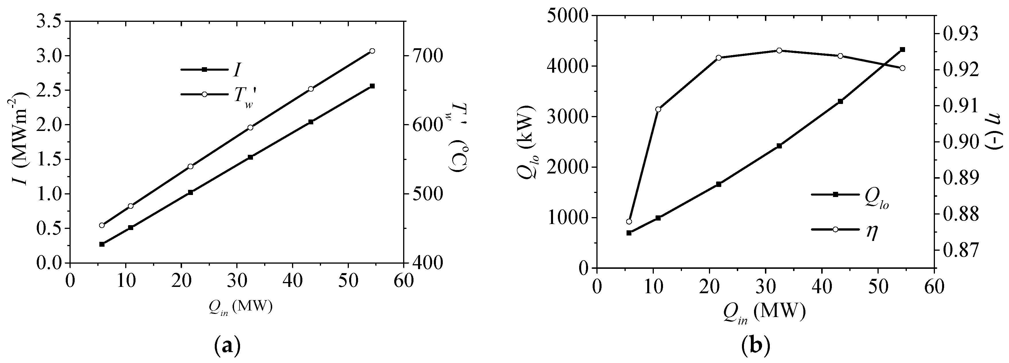
In order to obtain the absorbed energy power in a large range, the incident energy power should be changed. Figure 5 presents the heat transfer performance of the cavity receiver with different incident energy power. When the absorbed energy power increases from 5.0 MW to 50.0 MW as the incident power is increasing from 5.7 MW to 54.33 MW, the incident radiation flux remarkably rises from 0.269 MWm−2 to 2.56 MWm−2, and the surface temperature also sharply rises. When the incident energy power is increased, the heat loss remarkably rises, while the thermal efficiency will first increase and then decrease with the surface temperature rising. As MW, the maximum thermal efficiency reaches 92.53%.
The variations of the receiver area or incident energy power both mean the change of incident radiation flux. Figure 6 presents the thermal performance of the receiver under different incident radiation flux from Figure 3 and Figure 5. In general, the thermal performance of cavity receiver under different incident radiation flux by the change of receiver area or incident energy power is very similar.
As the incident radiation flux rises, thermal efficiency first increases and then decreases, as illustrated in Figure 6a. By maximizing the thermal efficiency, the optimal incident radiation flux 1.5 MWm−2 can be obtained. On the other hand, the inner wall temperature almost linearly increases with incident radiation flux. As a conclusion, the incident radiation flux is critically important for the thermal efficiency and wall temperature, and it is mainly dependent upon the receiver area and incident energy power as expressed in Equation (3). Under the present calculation conditions for the MSEE receiver, the inner wall temperature of receiver with optimal incident radiation flux 1.5 MWm−2 is 590 °C, and that is higher than the operating temperature range of molten salt. So, the molten salt cavity receiver with proper incident radiation flux should have high thermal efficiency, but the inner wall temperature adjacent to molten salt should be below the maximum operating temperature of this molten salt. Since the maximum operating temperature of solar salt is 565 °C, the optimal radiation flux for the solar salt cavity receiver is about 1.26 MWm−2.
Figure 7 presents the wall temperature difference and thermal efficiency of the receiver with different flow velocity, tube diameter and number of tubes in the receiver panel. By using the nonuniform heat transfer model, the receiver surface temperature is obviously higher than the wall temperature of the absorber tube in the back side . As the flow velocity increases from 0.5 ms−1 to 5.0 ms−1, the wall temperature difference remarkably drops from 128.45 °C to 32.03 °C, while the thermal efficiency can rise from 85.18% to 88.38%. As the tube diameter or number of tubes in the receiver panel is reduced, the flow velocity increases, and the thermal efficiency will rise due to the reduced wall temperature. Generally, the heat transfer inside the absorber tube can be enhanced by the increase of flow velocity or decrease of tube diameter and the number of tubes in the panel, and then the heat losses of convection and radiation are reduced with the decrease of receiver surface temperature, so the thermal efficiency can be enhanced.
Figure 8 presents the heat loss and thermal efficiency of the cavity receiver with different emissivity, insulation conductivity and wind velocity. If the emissivity of the selective coating is decreased from 1 to 0.1, the radiation heat loss remarkably decreases from 343.11 kW to 37.3 kW, while the other heat losses caused by convection and conduction changes very little, so the thermal efficiency increases from 86.78% to 91.83%. As the conductivity of the insulation layer decreases from 1 Wm−1K−1 to 0.05 Wm−1K−1, the conductive heat loss decreases from 80.21 kW to 6.08 kW, while the other heat losses have very little change, so the thermal efficiency increases from 86.67% to 87.88%. As the wind velocity decreases from 15 ms−1 to 1 ms−1, the heat loss caused by wind decreases from 214.99 kW to 24.65 kW, and then the thermal efficiency can be increased from 85.81% to 88.84%. In general, the decrease of emissivity, insulation conductivity and wind velocity can respectively reduce the heat losses of radiation, conduction and wind, while the other heat losses change very little, and then the thermal efficiency of the receiver gradually increases.
Figure 9 further presents the heat loss and energy proportion distributions under a different view factor. As the view factor or aperture area increases, the heat losses of reflection, radiation and convection totally rise, because larger aperture has larger heat loss through convection and radiation. On the other hand, conductive heat loss only changes very little with a constant receiver area. When the view factor rises from 0.1 to 1, the reflective heat loss increases from 20.77 kW to 229.88 kW, and the radiation heat loss increases from 36.74 kW to 301.38 kW, while the convective heat loss increases from 123.08 kW to 204.03 kW. As a result, the energy proportions of radiation and reflection remarkably rises for 6.40 and 8.98 times, while the energy proportion of conduction varies within 0.21–0.23%, and the thermal efficiency decreases from 96.29% to 87.01%.
According to the previous calculation results, the incident radiation flux caused by the receiver area and incident energy power plays the primary role in the heat transfer of cavity receiver. The thermal efficiency will approach to maximum at the optimal incident radiation flux, while the inner wall temperature with high incident radiation flux will be probably beyond the operating temperature of molten salt, so the proper incident radiation flux is very important for the high thermal efficiency receiver. The increase of flow velocity or decrease of tube diameter and number of tubes in panel can increase the thermal efficiency of cavity receiver and decrease the wall temperature difference, but the pumping power consumption will be also remarkably increased.
The decrease of surface emissivity can remarkably benefit the receiver efficiency, while the insulation layer only affects the receiver efficiency very little. In addition, the decrease of the view factor or aperture can increase the thermal efficiency, but a too small aperture will reduce the incident energy power.
4. Heat Transfer Performance with Variable Fluid Temperature
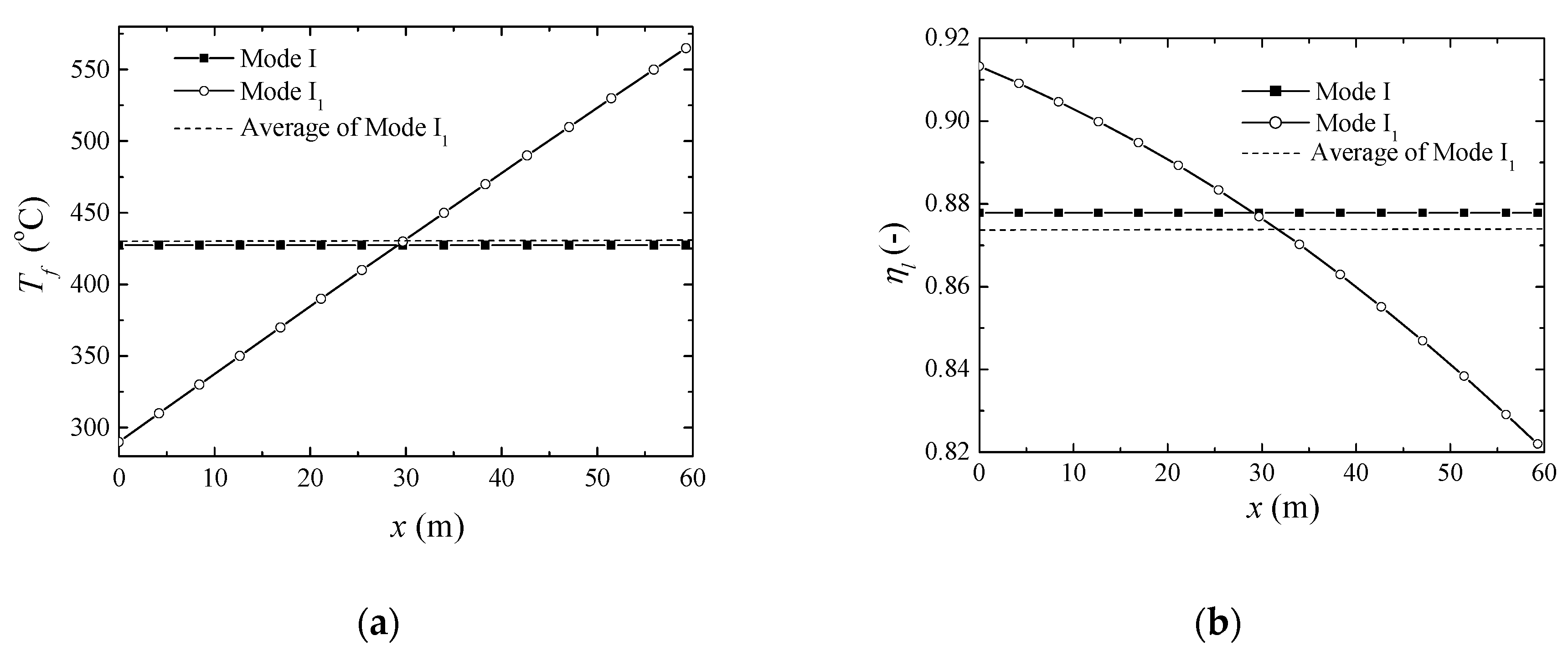
In the previous section, the cavity receiver was designed by average bulk temperature based on inlet and outlet values (427.5 °C) and absorbed energy power (5 MW), and the calculation results of MSEE by Mode I are described as Table 1. For a practical cavity receiver, the fluid temperature gradually increases from the inlet temperature to the outlet temperature, and then the thermal efficiency also changes. In addition, the heat transfer performance along the absorber tube ( °C) will be further calculated by the incident energy power from Mode I ( MW), and this calculation mode is defined as Mode I1. Figure 10 further presents the fluid temperature and thermal efficiency along the receiver calculated by Mode I and I1. Along the flow direction, the fluid temperature almost linearly increases, while the thermal efficiency gradually decreases. According to the calculation results in Table 2, the average fluid temperature along the receiver by Mode I1 is a little higher than that in Mode I, while the average thermal efficiency along the absorber tube by Mode I1 is lower than that by Mode I for higher heat loss. According to Figure 10, the whole length of the receiver tube from inlet to outlet should be about 59.3 m, and L/d = 3778. The height of the typical receiver is 6 m, and H/d = 382.
Because the average thermal efficiency along the receiver calculated by Mode I1 is 0.41% lower than that by Mode I, the absorbed energy power 4.977 MW is less than the required energy power 5.000 MW. In order to obtain the required energy power 5 MW, the cavity receiver should be recalculated, and this calculation mode is defined as Mode II with incident energy power 5.720 MW, as illustrated in Table 2. Figure 11 further presents the fluid temperature and thermal efficiency along the receiver calculated by Mode II. Along the flow direction, the fluid temperature and surface temperature almost linearly increase, while the thermal efficiency gradually decreases. At the inlet, the thermal efficiency is as high as 91.34% with the fluid temperature of 290 °C, while it decreases to 82.25% at the outlet.
In general, the calculated heat transfer performance by Mode II in Figure 11 is similar to those by Mode I1 in Figure 10, and the detailed results are presented in Table 2. By considering variable fluid temperature along the receiver tube in Mode II, the average fluid temperature 429 °C is higher than the average of inlet and outlet temperature 427.5 °C, because the temperature distribution function along the flow direction is a convex function. As a result, the average thermal efficiency 87.41% in Mode II is lower than the thermal efficiency calculated by the average of inlet and outlet temperature for 0.38%.
5. Heat Transfer Performance with Variable Circumferential Temperature
Because the incident energy flux changes along the front semi-circumference of the receiver tube from Equation (28), the circumferential heat transfer performance is also uneven. In this section, the heat transfer along the circumference is first calculated by the incident energy power from Mode I (, MW) and the average arithmetic fluid temperature ( °C), and this calculation mode is defined as Mode I2. From Table 3, the absorbed energy power 4.973 MW calculated by Mode I2 is less than the required energy power 5.000 MW. In order to obtain the required energy power 5 MW, the cavity receiver should be recalculated by the incident energy power 5.728 MW, and this calculation mode is defined as Mode III. By considering the variable circumferential temperature, the average thermal efficiency along the circumference calculated by Mode III is 87.29%, and that is lower than that calculated by Mode I.
Figure 12a presents the incident energy flux and absorbed energy flux along the front semi-circumference calculated by Mode III. As the incident angle increases from 0° to 90°, the absorbed energy flux decreases with the incident energy flux, and their difference or the heat loss also significantly drops. As the incident angle is zero, the incident energy flux and absorbed energy flux reach the maxima of 0.270 MW−2 and 0.239 MW−2. Figure 12b further presents the local wall temperature and thermal efficiency along the circumference calculated by Mode III. The wall temperature first gradually decreases near the perpendicularly incident region, and then linearly drops, while the maximum temperature difference along the circumference is 83.62 °C. As the incident angle increases, the thermal efficiency first approaches to the maximum 88.3% at the perpendicularly incident point, and then it gradually decreases and final sharply drops near the parallelly incident region.
6. Receiver with Variable Circumferential Temperature and Fluid Temperature
According to previous investigation, nonuniform heat transfer caused by variable fluid temperature or variable circumferential temperature can decrease the thermal efficiency of the cavity receiver for higher heat loss. In this section, the heat transfer of the receiver is calculated with variable circumferential temperature and variable fluid temperature, and this calculation mode is defined as Mode IV. Table 4 presents the heat transfer performance of the cavity receiver calculated by different modes of a nonuniform heat transfer model. By considering variable circumferential temperature and variable fluid temperature, the thermal efficiency of the cavity receiver is lower than that calculated by Mode II (variable fluid temperature) or Mode III (variable circumferential temperature), and that calculated by Mode I (uniform circumferential temperature and fluid temperature) is highest. The thermal efficiency of cavity receiver calculated by Mode IV is 86.93%, and that is also close to experimental result.
Figure 13a presents the local wall temperature along the circumference under different fluid temperature calculated by Mode IV. The wall temperature distribution under different fluid temperature is very similar, and it gradually decreases with incident angle rising. Along the flow direction, both the fluid temperature and wall temperature increase, and the maximum wall temperature at the outlet of receiver ( °C) reaches 637.5 °C at the perpendicularly incident point. Figure 13b further presents the local thermal efficiency along the circumference under different fluid temperature calculated by Mode IV. The local thermal efficiency distribution under different fluid temperature is also similar. As the incident angle increases, the thermal efficiency first reaches the maximum at the perpendicularly incident point, and then it gradually decreases and finally sharply drops near the parallelly incident region. Along the flow direction, the thermal efficiency decreases with fluid temperature increasing. At the inlet of receiver ( °C), the thermal efficiency reaches as high as 91.6% at the perpendicularly incident point. At the outlet of receiver ( °C), the thermal efficiency at the perpendicularly incident point decreases to 82.9%, while the average thermal efficiency along the circumference is 81.78% for high heat loss at high temperature.
7. Conclusions and Discussions
In this paper, the nonuniform heat transfer model of the cavity receiver is established by considering the circular tube structure, variable fluid temperature and variable circumferential temperature, and then the thermal performance of the molten salt cavity receiver is further analyzed. The thermal efficiency of the cavity receiver MSEE calculated by the nonuniform model is 86.93–87.79%, and that fit very well with the experimental result. Because of nonuniform heat transfer, wall and fluid temperatures have large differences, and then the thermal efficiency of the cavity receiver calculated by variable fluid temperature or variable circumferential temperature is lower. The thermal efficiency of the cavity receiver calculated by variable fluid temperature and variable circumferential temperature is lower than that calculated by average fluid temperature and bilateral uniform circumferential temperature for 0.86%.
The incident radiation flux caused by the receiver area and incident energy power plays a primary role in heat transfer of the cavity receiver. As incident radiation flux rises, thermal efficiency first increases and then decreases, and the cavity receiver with incident radiation flux of 1.5 MWm−2 has maximum thermal efficiency. For the solar salt cavity receiver, the optimal radiation flux is 1.26 MWm−2 for the operating temperature limit of solar salt. The thermal efficiency of the receiver can be increased by heat convection enhancement with the increase of flow velocity or decrease of tube diameter and number of tubes in the panel. The decrease of view factor can increase thermal efficiency by reducing the convection and radiation heat loss, and the decrease of surface emissivity and insulation conductivity can respectively reduce the radiation and conductive heat loss.
This article establishes a novel nonuniform heat transfer model for cavity receiver, and then associated thermal performance and optimal/enhanced parameter can be analyzed. These results can be applied for the structure design and parameter choice of molten salt cavity receiver in solar thermal power. In this article, the cavity receiver calculation is limited by the assumption of uniform incident radiation flux, and the associated model and research can be further improved by considering nonuniform radiation flux, complex cavity structure and other heat transfer fluid.
Author Contributions
Investigation-writing, J.L.; editing, Y.W.; project administration, J.D. All authors have read and agreed to the published version of the manuscript.
Funding
This paper is supported by National Natural Science Foundation of China (U1601215, 51961165101) and Natural Science Foundation of Guangdong Province (2017B030308004).
Conflicts of Interest
The authors declare no conflict of interest.
References
- Llamas, J.; Martín, D.B.; De Adana, R.; De Adana, M.R. Optimization of 100 MWe Parabolic-Trough Solar-Thermal Power Plants Under Regulated and Deregulated Electricity Market Conditions. Energies 2019, 12, 3973. [Google Scholar] [CrossRef] [Green Version]
- Ortega, J.I.; Burgaleta, J.I.; Téllez, F.M. Central Receiver System Solar Power Plant Using Molten Salt as Heat Transfer Fluid. J. Sol. Energy Eng. 2008, 130, 024501. [Google Scholar] [CrossRef]
- Radosevich, L.G.; Skinrood, A.C. The Power Production Operation of Solar One, the 10 MWe Solar Thermal Central Receiver Pilot Plant. J. Sol. Energy Eng. 1989, 111, 144–151. [Google Scholar] [CrossRef]
- Epstein, M.; Liebermann, D.; Rosh, M.; Shor, A.J. Solar testing of 2MWt water/steam receiver at the Weizmann Institutse solar tower. Solar Energy Mater. 1991, 24, 265–278. [Google Scholar] [CrossRef]
- Litwin, R.Z.; Rogers, R.D.O. Fabrication and Installation of the Solar Two Central Receiver; ASME Solar Engineering: New York, USA, USA, 1996; pp. 125–132. [Google Scholar]
- Ávila-Marín, A.L. Volumetric receivers in Solar Thermal Power Plants with Central Receiver System technology: A review. Sol. Energy 2011, 85, 891–910. [Google Scholar] [CrossRef]
- Clausing, A. An analysis of convective losses from cavity solar central receivers. Sol. Energy 1981, 27, 295–300. [Google Scholar] [CrossRef]
- Reddy, K.; Kumar, N.S. Combined laminar natural convection and surface radiation heat transfer in a modified cavity receiver of solar parabolic dish. Int. J. Therm. Sci. 2008, 47, 1647–1657. [Google Scholar] [CrossRef]
- Prakash, M.; Kedare, S.; Nayak, J. Investigations on heat losses from a solar cavity receiver. Sol. Energy 2009, 83, 157–170. [Google Scholar] [CrossRef]
- Cui, F.; He, Y.; Cheng, Z.-D.; Li, Y. Study on combined heat loss of a dish receiver with quartz glass cover. Appl. Energy 2013, 112, 690–696. [Google Scholar] [CrossRef]
- Wang, Q.; Wang, J.; Tang, R. Design and Optical Performance of Compound Parabolic Solar Concentrators with Evacuated Tube as Receivers. Energies 2016, 9, 795. [Google Scholar] [CrossRef] [Green Version]
- Msaddak, A.; Sediki, E.; Ben Salah, M. Assessment of thermal heat loss from solar cavity receiver with Lattice Boltzmann method. Sol. Energy 2018, 173, 1115–1125. [Google Scholar] [CrossRef]
- Hoffman, H.W.; Cohen, S.I. Fused Salt Heat Transfer Part III: Forced Convection Heat Transfer in Circular Tubes Containing the Salt Mixture NaNO2-KNO3-NaNO3. Report No. ORNL-2433; 1960; pp. 9–13. Available online: https://www.osti.gov/servlets/purl/4181833 (accessed on 12 October 2019).
- Silverman, M.D.; Huntley, W.R.; Robertson, H.E. Heat Transfer Measurements in a Forced Convection Loop with Two Molten-Fluoride Salts: LiF-BeF2-ThF4-UF4 and EUTECTIC NaBF4-NaF. 1976, pp. 16–21. Available online: https://inis.iaea.org/collection/NCLCollectionStore/_Public/08/296/8296902.pdf (accessed on 15 October 2019).
- Lu, J.F.; Shen, X.Y.; Ding, J.; Peng, Q.; Wen, Y.L. Convective heat transfer of high temperature molten salt in transversely grooved tube. Appl. Therm. Eng. 2013, 61, 157–162. [Google Scholar]
- Lu, J.; Ding, J.; Yu, T.; Shen, X. Enhanced heat transfer performances of molten salt receiver with spirally grooved pipe. Appl. Therm. Eng. 2015, 88, 491–498. [Google Scholar] [CrossRef]
- Liu, J.; He, Y.; Lei, X. Heat-Transfer Characteristics of Liquid Sodium in a Solar Receiver Tube with a Nonuniform Heat Flux. Energies 2019, 12, 1432. [Google Scholar] [CrossRef] [Green Version]
- Neber, M.; Lee, H. Design of a high temperature cavity receiver for residential scale concentrated solar power. Energy 2012, 47, 481–487. [Google Scholar] [CrossRef]
- Steinfeld, A.; Schubnell, M. Optimum aperture size and operating temperature of a solar cavity-receiver. Sol. Energy 1993, 50, 19–25. [Google Scholar] [CrossRef]
- Montes, M.J.; Rovira, A.; Martínez-Val, J.; Ramos, Á. Proposal of a fluid flow layout to improve the heat transfer in the active absorber surface of solar central cavity receivers. Appl. Therm. Eng. 2012, 35, 220–232. [Google Scholar] [CrossRef]
- Le Roux, W.; Bello-Ochende, T.; Meyer, J. Operating conditions of an open and direct solar thermal Brayton cycle with optimised cavity receiver and recuperator. Energy 2011, 36, 6027–6036. [Google Scholar] [CrossRef] [Green Version]
- Albarbar, A.; Arar, A. Performance Assessment and Improvement of Central Receivers Used for Solar Thermal Plants. Energies 2019, 12, 3079. [Google Scholar] [CrossRef] [Green Version]
- Jiang, K.; Du, X.; Kong, Y.; Xu, C.; Ju, X. A comprehensive review on solid particle receivers of concentrated solar power. Renew. Sustain. Energy Rev. 2019, 116, 109463. [Google Scholar] [CrossRef]
- Nie, F.; Cui, Z.; Bai, F.; Wang, Z. Properties of solid particles as heat transfer fluid in a gravity driven moving bed solar receiver. Sol. Energy Mater. Sol. Cells 2019, 200, 110007. [Google Scholar] [CrossRef]
- Sarafraz, M.M.; Arjomandi, M. Demonstration of plausible application of gallium nano-suspension in microchannel solar thermal receiver: Experimental assessment of thermo-hydraulic performance of microchannel. Int. Commun. Heat Mass Transf. 2018, 94, 39–46. [Google Scholar] [CrossRef]
- Sarafraz, M.M.; Arya, H.; Arjomandi, M. Thermal and hydraulic analysis of a rectangular microchannel with gallium-copper oxide nano-suspension. J. Mol. Liq. 2018, 263, 382–389. [Google Scholar] [CrossRef]
- Sedighi, M.; Taylor, R.A.; Lake, M.; Rose, A.; Izadgoshasb, I.; Padilla, R.V. Development of a novel high-temperature, pressurised, indirectly-irradiated cavity receiver. Energy Convers. Manag. 2020, 204, 112175. [Google Scholar] [CrossRef]
- Yu, T.; Yuan, Q.; Lu, J.; Ding, J.; Lu, Y. Thermochemical storage performances of methane reforming with carbon dioxide in tubular and semi-cavity reactors heated by a solar dish system. Appl. Energy 2017, 185, 1994–2004. [Google Scholar] [CrossRef]
- Corgnale, C.; Ma, Z.; Shimpalee, S. Modeling of a direct solar receiver reactor for decomposition of sulfuric acid in thermochemical hydrogen production cycles. Int. J. Hydrogen Energy 2019, 44, 27237–27247. [Google Scholar] [CrossRef]
- Duniam, S.; Jahn, I.; Hooman, K.; Lu, Y.; Veeraragavan, A. Comparison of direct and indirect natural draft dry cooling tower cooling of the sCO2 Brayton cycle for concentrated solar power plants. Appl. Therm. Eng. 2018, 130, 1070–1080. [Google Scholar] [CrossRef]
- Guo, J.-Q.; Li, M.-J.; Xu, J.; Yan, J.; Wang, K. Thermodynamic performance analysis of different supercritical Brayton cycles using CO2-based binary mixtures in the molten salt solar power tower systems. Energy 2019, 173, 785–798. [Google Scholar] [CrossRef]
- Goodarzi, H.; Akbari, O.A.; Sarafraz, M.M.; Karchegani, M.M.; Safaei, M.R.; Shabani, G.A.S.; Mokhtari, M. Numerical Simulation of Natural Convection Heat Transfer of Nanofluid With Cu, MWCNT, and Al2O3 Nanoparticles in a Cavity With Different Aspect Ratios. J. Therm. Sci. Eng. Appl. 2019, 11, 061020-8. [Google Scholar] [CrossRef]
- Sarafraz, M.M.; Safaei, M.R. Diurnal thermal evaluation of an evacuated tube solar collector (ETSC) charged with graphene nanoplatelets-methanol nano-suspension. Renew. Energy 2019, 142, 364–372. [Google Scholar] [CrossRef]
- Li, X.; Kong, W.; Wang, Z.; Chang, C.; Bai, F. Thermal model and thermodynamic performance of molten salt cavity receiver. Renew. Energy 2010, 35, 981–988. [Google Scholar] [CrossRef]
- Winter, C.J.; Sizmann, R.L.; Vant-hull, L.L. Solar Power Plants-Fundamentals, Technology Systems and Economics; Springer: Berlin, Germany, 1991. [Google Scholar]
- Crump, J.R. A heat transfer textbook by John H. Lienhard, prentice hall, 1981, 51 6+ xi pages; price$24.95. AIChE J. 1981, 27, 700. [Google Scholar] [CrossRef]
- Siebers, D.L.; Kraabel, J.S. Estimating convective energy losses from solar central receivers. Sand 1984, 17, 84–87. [Google Scholar]
- Lu, J.F.; Ding, J.; Yang, J.P. Heat transfer performance of the receiver pipe under unilateral concentrated solar radiation. Solar Energy 2010, 84, 1879–1887. [Google Scholar]
- Colburn, A.P. A method of correlating forced convection heat-transfer data and a comparison with fluid friction. Int. J. Heat Mass Transf. 1964, 7, 1359–1384. [Google Scholar] [CrossRef]
- Bergan, N.E. An external molten salt solar central receiver test. Solar Eng. 1987, 1, 474–478. [Google Scholar]
- Zavoico, A.B. Solar Power Tower Design Basis Document. Report No. SAND2001-2100; Sandia National Laboratories, 2001. Available online: https://www.osti.gov/biblio/786629-solar-power-tower-design-basis-document-revision (accessed on 5 November 2019).
Figure 1.
Basic structure and heat absorption model of cavity receiver.

Figure 2.
The basic thermal resistance model of the cavity receiver is the surrounding temperature; and are the receiver surface temperature and inner wall temperature in front side; is fluid temperature, and are the receiver outer wall temperature and inner wall temperature in back side; and is outer wall temperature of insulation layer.

Figure 3.
Heat absorption performance of the receiver with a different receiver area: (a) incident radiation flux and surface temperature; (b) heat loss and thermal efficiency.
Figure 3.
Heat absorption performance of the receiver with a different receiver area: (a) incident radiation flux and surface temperature; (b) heat loss and thermal efficiency.

Figure 4.
Heat loss of receiver with different receiver area: (a) Heat loss; (b) Heat loss proportion.
Figure 4.
Heat loss of receiver with different receiver area: (a) Heat loss; (b) Heat loss proportion.

Figure 5.
Heat absorption performance of the receiver under different incident energy power: (a) incident radiation flux and surface temperature; (b) heat loss and thermal efficiency.
Figure 5.
Heat absorption performance of the receiver under different incident energy power: (a) incident radiation flux and surface temperature; (b) heat loss and thermal efficiency.

Figure 6.
Thermal performance of receiver with different incident radiation flux: (a) Thermal efficiency; (b) Inner wall temperature.
Figure 6.
Thermal performance of receiver with different incident radiation flux: (a) Thermal efficiency; (b) Inner wall temperature.

Figure 7.
Temperature difference and thermal efficiency of receiver with different flow velocity, tube diameter and number of tubes in panel: (a) Flow velocity; (b) Tube diameter; (c) Number of tubes in panel.
Figure 7.
Temperature difference and thermal efficiency of receiver with different flow velocity, tube diameter and number of tubes in panel: (a) Flow velocity; (b) Tube diameter; (c) Number of tubes in panel.

Figure 8.
Heat loss and thermal efficiency of receiver with different emissivity, insulation conductivity, and wind velocity: (a) Emissivity; (b) Insulation conductivity; (c) Wind velocity.
Figure 8.
Heat loss and thermal efficiency of receiver with different emissivity, insulation conductivity, and wind velocity: (a) Emissivity; (b) Insulation conductivity; (c) Wind velocity.

Figure 9.
Heat loss and energy proportion distributions with different view factor: (a) heat loss; (b) Energy proportion.
Figure 9.
Heat loss and energy proportion distributions with different view factor: (a) heat loss; (b) Energy proportion.

Figure 10.
Temperature and thermal efficiency along absorber tube calculated by Mode I and I1: (a) Fluid temperature; (b) Thermal efficiency.
Figure 10.
Temperature and thermal efficiency along absorber tube calculated by Mode I and I1: (a) Fluid temperature; (b) Thermal efficiency.

Figure 11.
Temperature and thermal efficiency along absorber tube calculated by Mode II.

Figure 12.
Heat transfer performance along the circumference calculated by Mode III: (a) incident and absorbed energy fluxes, (b) wall temperature and thermal efficiency.
Figure 12.
Heat transfer performance along the circumference calculated by Mode III: (a) incident and absorbed energy fluxes, (b) wall temperature and thermal efficiency.

Figure 13.
The heat transfer performance along the circumference under different fluid temperature calculated by Mode IV: (a) wall temperature, (b) thermal efficiency.
Figure 13.
The heat transfer performance along the circumference under different fluid temperature calculated by Mode IV: (a) wall temperature, (b) thermal efficiency.


Table 1.
Heat transfer performance of the cavity receiver calculated by a uniform and nonuniform model (Mode I).
Table 1.
Heat transfer performance of the cavity receiver calculated by a uniform and nonuniform model (Mode I).
| Parameter | Uniform (Mode l) | Nonuniform (Mode l) | Difference | Relative Difference (%) |
|---|---|---|---|---|
| (°C) | 427.50 | 427.50 | - | - |
| (MW) | 5.000 | 5.000 | - | - |
| Tw (°C) | 508.62 | 479.12 | −29.5 | −5.80 |
| Tbw (°C) | 508.62 | 427.1 | −81.52 | −16.0 |
| (MW) | 5.758 | 5.696 | −0.062 | −1.08 |
| (%) | 86.84 | 87.79 | 0.95 | 1.09 |
| (MW) | 0.758 | 0.696 | −0.062 | −8.18 |
| (MW) | 0.327 | 0.279 | −0.048 | −14.7 |
| (MW) | 0.115 | 0.107 | −0.008 | −6.96 |
| (MW) | 0.094 | 0.089 | −0.005 | −5.32 |
| (MW) | 0.209 | 0.207 | −0.002 | −0.96 |
Mode I: Nonuniform heat transfer model with average fluid temperature and bilateral uniform circumferential temperature ( °C, MW).
Table 2.
Heat transfer performance comparison with average fluid temperature and variable fluid temperature.
Table 2.
Heat transfer performance comparison with average fluid temperature and variable fluid temperature.
| Parameter | Mode I | Mode I1 | Mode II |
|---|---|---|---|
| (MW) | 5.696 | 5.696 | 5.720 |
| (MWm−2) | 0.2687 | 0.2687 | 0.2698 |
| (°C) | 427.50 | 429.01 | 429.00 |
| (°C) | 479.12 | 482.06 | 482.29 |
| (MW) | 0.696 | 0.719 | 0.720 |
| (MW) | 5.000 | 4.977 | 5.000 |
| (%) | 87.79 | 87.38 | 87.41 |
Mode I1: Nonuniform heat transfer model with variable fluid temperature, bilateral uniform circumferential temperature and incident energy power from Mode I ( °C, ); Mode II: Nonuniform heat transfer model with variable fluid temperature and bilateral uniform circumferential temperature ( °C, MW).
Table 3.
Heat transfer performance comparison with bilateral uniform wall temperature and variable circumferential temperature.
Table 3.
Heat transfer performance comparison with bilateral uniform wall temperature and variable circumferential temperature.
| Parameter | Mode I | Mode I2 | Mode III |
|---|---|---|---|
| (MW) | 5.696 | 5.696 | 5.728 |
| (MWm−2) | 0.2687 | 0.2687 | 0.2698 |
| (°C) | 427.50 | 427.50 | 427.50 |
| (°C) | 479.12 | 478.88 | 479.19 |
| (MW) | 0.696 | 0.723 | 0.728 |
| (MW) | 5.000 | 4.973 | 5.000 |
| (%) | 87.79 | 87.31 | 87.29 |
Mode I2: Nonuniform heat transfer model with average fluid temperature, variable circumferential temperature and incident energy power from Mode I ( °C, , ); Mode III: Nonuniform heat transfer model with average fluid temperature and variable circumferential temperature ( °C, , MW).
Table 4.
Heat transfer performance of cavity receiver calculated by different modes of nonuniform model (Mode I–IV).
Table 4.
Heat transfer performance of cavity receiver calculated by different modes of nonuniform model (Mode I–IV).
| Parameter | Mode I | Mode I1 | Mode II | Mode IV |
|---|---|---|---|---|
| (MW) | 5.696 | 5.720 | 5.728 | 5.752 |
| (MWm−2) | 0.2687 | 0.2698 | 0.2698 | 0.2713 |
| (°C) | 427.50 | 429.00 | 427.50 | 429.87 |
| (°C) | 479.12 | 482.29 | 479.19 | 483.18 |
| (MW) | 0.696 | 0.720 | 0.728 | 0.752 |
| (MW) | 5.000 | 5.000 | 5.000 | 5.000 |
| (%) | 87.79 | 87.41 | 87.29 | 86.93 |
Mode IV: Nonuniform heat transfer model with variable fluid temperature and variable circumferential temperature ( °C, , MW).
© 2020 by the authors. Licensee MDPI, Basel, Switzerland. This article is an open access article distributed under the terms and conditions of the Creative Commons Attribution (CC BY) license (http://creativecommons.org/licenses/by/4.0/).
Share and Cite
MDPI and ACS Style
Lu, J.; Wang, Y.; Ding, J. Nonuniform Heat Transfer Model and Performance of Molten Salt Cavity Receiver. Energies 2020, 13, 1001. https://0-doi-org.brum.beds.ac.uk/10.3390/en13041001
AMA Style
Lu J, Wang Y, Ding J. Nonuniform Heat Transfer Model and Performance of Molten Salt Cavity Receiver. Energies. 2020; 13(4):1001. https://0-doi-org.brum.beds.ac.uk/10.3390/en13041001
Chicago/Turabian StyleLu, Jianfeng, Yarong Wang, and Jing Ding. 2020. "Nonuniform Heat Transfer Model and Performance of Molten Salt Cavity Receiver" Energies 13, no. 4: 1001. https://0-doi-org.brum.beds.ac.uk/10.3390/en13041001
Note that from the first issue of 2016, this journal uses article numbers instead of page numbers. See further details here.