Management and Activation of Energy Flexibility at Building and Market Level: A Residential Case Study

Abstract

The electricity sector foresees a significant change in the way energy is generated and distributed in the coming years. With the increasing penetration of renewable energy sources, smart algorithms can determine the difference about how and when energy is produced or consumed by residential districts. However, managing and implementing energy demand response, in particular energy flexibility activations, in real case studies still presents issues to be solved. This study, within the framework of the European project “SABINA H2020”, addresses the development of a multi-level optimization algorithm that has been tested in a semi-virtual real-time configuration. Results from a two-day test show the potential of building’s flexibility and highlight its complexity. Results show how the first level algorithm goal to reduce the energy injected to the grid is accomplished as well as the energy consumption shift from nighttime to daytime hours. As conclusion, the study demonstrates the feasibility of such kind of configurations and puts the basis for real test site implementation.

1. Introduction

The decarbonization of the electricity grid goes in hand with the penetration of renewable power sources. In recent years, big renewable power generation plants have represented the majority of renewable power sources [1], however, a significant change is under way in the traditional paradigms of the electricity sector. Electricity is no longer generated only in centralized power plants and consumed by final users but, instead, it is being generated in many places at lower power rates as distributed resources. Moreover, the inherent variability of renewable generation from dispersed small producers together with the fluctuation in the consumption opens the door to additional opportunities in grid balancing. In fact, now that generation is dispersing, grid balancing could be too, giving space to local actors, such as consumers, to participate in the balancing markets. To do so, consumers should be capable to modify their consumption and generation patterns reacting to the requirement of the grid, becoming “prosumers”. This is called demand response (DR), which is gaining relevance in the whole system and should be considered in the nearby future for energy distribution and management [2].

However, balancing markets throughout Europe have several requirements, such as the bidding size, that act as barriers for small prosumers [3]. Thus, if small buildings want to participate in these markets, they need to act in harmonized and coordinated ways to overcome such limitations. This coordination role falls within the responsibility of a demand aggregator (DA).

For their stochastic uncertainty [4], the lower energy and power rates of individual buildings and the immense differences between buildings, DA of residential districts has not been targeted from a business perspective by existing DA in EU, who generally tend to consider big or intermediate industries, commercial or tertiary buildings [5,6].

In the case of residential districts, the DA gathers the energy from several prosumers allowing them to participate in balancing energy markets by shifting the energy consumption from one period to another.

Nonetheless, these prosumers need some kind of intelligence to be part of a smart grid. First, to be able to optimize and manage the energy loads and resources inside the building. Second, to be able to interact with the DA and provide the expected response.

Energy flowing through electric elements, such as batteries, appliances or electric vehicle is relatively simple to model, however, the majority of the consumption of residential buildings comes from the heating and cooling systems. Investigating the potentiality of thermal mass to act as an additional distributed resource to store energy for further use in the building was seen as an opportunity to be investigated by the SABINA H2020 project [7]. SABINA has the main objective to enhance the penetration of renewable power sources in the electricity grid through building flexibility.

This study presents how the SABINA project addressed this intelligence challenge by developing a multi-level optimization process in a semi-virtual building. These levels are related to the global functionality or semi-independent goals of the whole project, which pretend to enhance (maximize) the in-house use of renewable energy sources (RES) and to reduce the greenhouse gas (GHG) emissions caused by the energy consumption of residential buildings.

At the first level, a building algorithm (BA) aims at maximizing the self-consumption of the RES managing the energy consumption/generation of all the elements within the building. At the second level, the Market Integrated District Algorithm (MIDA) is responsible of the interaction and coordination of the buildings with the electricity grid so they can participate in balancing energy markets. In particular, the main driver to decide what to do in MIDA is the grid electricity mix, as it tackles to reduce the GHG emissions, knowing that not only economic factors should be expected from demand aggregators [8].

Another key point is the necessity to test these complex systems in order to further demonstrate the benefits and the feasibility of these kind of approaches. The first stage of SABINA project is to test the whole configuration under controlled laboratory conditions. This is necessary to validate all the subsystems and algorithms before applying the approach on real test sites.

This paper presents the integration of both algorithms, their interactions, the configuration of the whole system and the actors involved. Then, the study presents the energy flexibility results and system performance during a two-day experiment in one of the testing laboratories at the IREC facilities (Energy SmartLab).

The remainder of the paper is organized as follows: Section 2 describes the whole system, the laboratory equipment involved, the relations between all the actors involved the algorithms and the building model used. Section 3 presents the results and we end with the conclusions of the work in Section 4.

2. Material and Methods

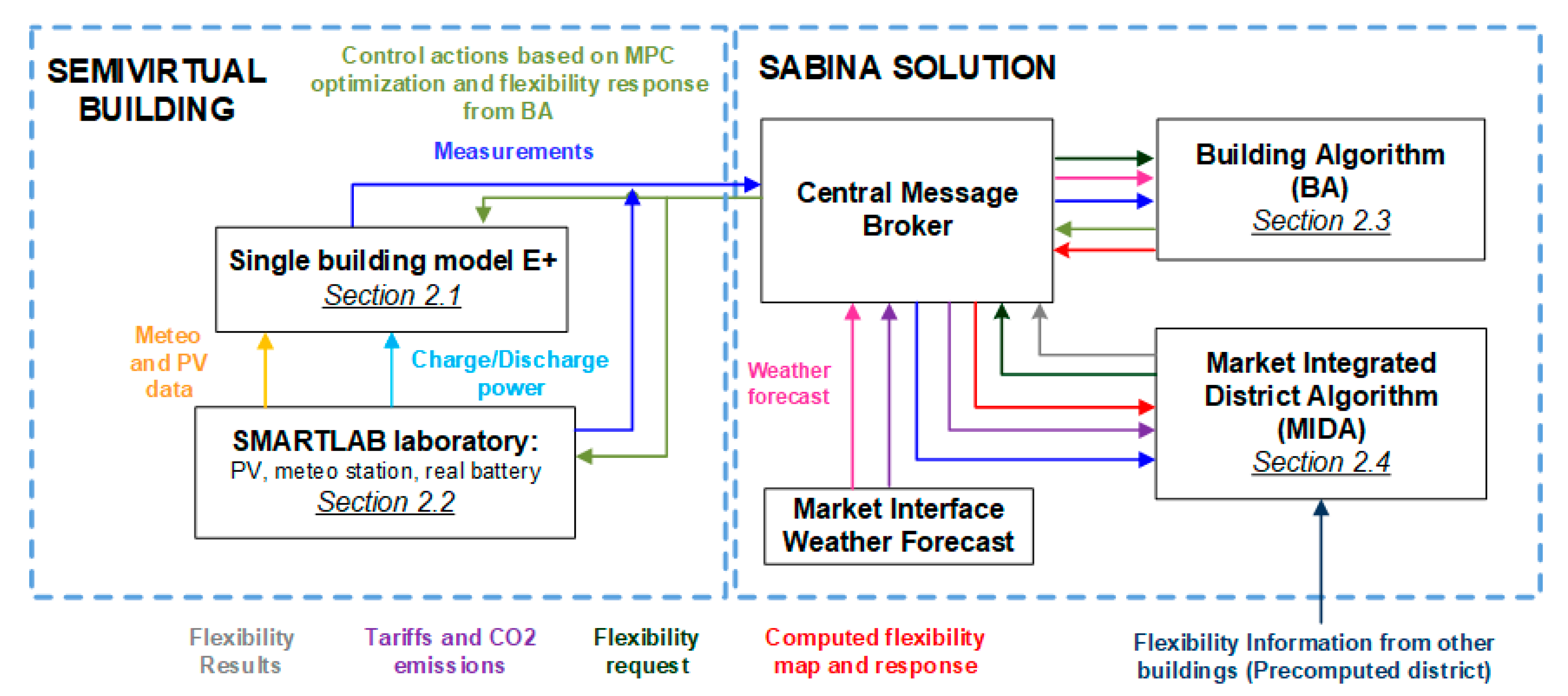
As mentioned in the introduction, the study is based in a semi-virtual building. This means that, instead of a building, what the project works with is a simulated building that has some real elements that run in real-time in IREC’s laboratories. Therefore, the overall system should be understood as the semi-virtual building that respond to the SABINA solution. As shown in Figure 1, the SABINA solution consists of a central broker that gathers and stores the information from two main concepts. For one side there are the inherent elements involved: Market Interface (MI), Weather Forecast, the BA and the MIDA. For the other side, there is the semi-virtual building, which is composed of the single building model (created using EnergyPlus) and the real equipment in the SmartLab laboratory. These elements pick and send information from and to the central broker when needed. All these elements are explained in more depth in Section 2.1, Section 2.2, Section 2.3 and Section 2.4 to have a clear picture of what each element works for and how it interacts with the rest of elements.

With this configuration (Figure 1), the addition of buildings can be easily performed without changing the SABINA solution. The following sub-sections describe each one of the aforementioned elements involved to better understand the overall system.

2.1. Building Model E+

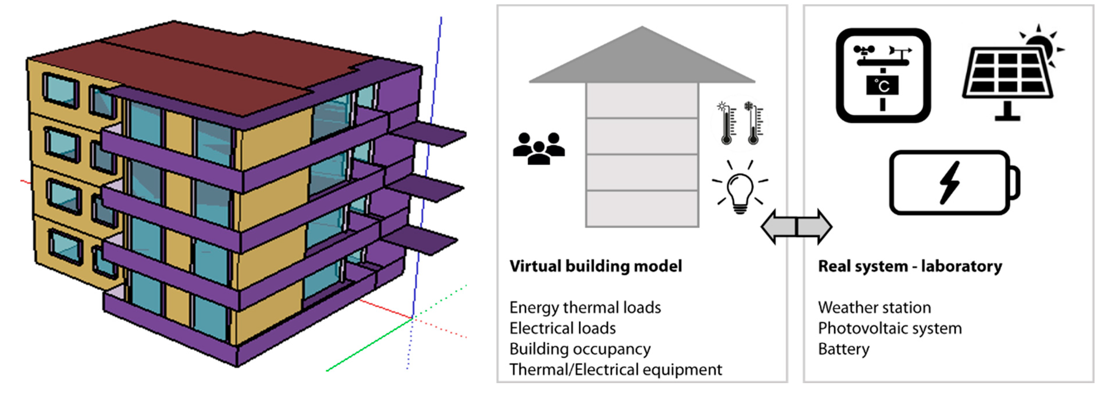
The residential case study represents a four-floor building located in Tarragona, Spain. It is representative of the Spanish building stock of the period from 1991 to 2007 and it follows the building code NRE-AT-87, which building typology is described by Tejero et al. [9]. It consists in four identical dwellings (one per floor), each divided in two thermal zones with different occupancy patterns. Moreover, occupancy profiles are stochastic as well as appliances and lighting consumption. In terms of energy demands, this approach leads to relatively high variability between dwellings and it simulates a system close to the reality where people’s behavior, especially in the residential sector, is hard to predict [10]. Domestic hot water (DHW) tapping profiles are based on the European standard (EN16147, 2011) and they have been adjusted according to building occupancy. Regarding space heating (SH) and DHW production, individual air-to-water heat pumps represent the main heating source. This system provides hot water for the indoor fan coil units (two units per dwelling) and the DHW. Room thermostats with a control dead band of 0.5 °C manage fan coils operation.

The building has a PV installation on the rooftop that has a peak power of 10.8 kW. Additionally, the building is equipped with a 10 kWh community battery installed to ease the storage of PV generation surplus.

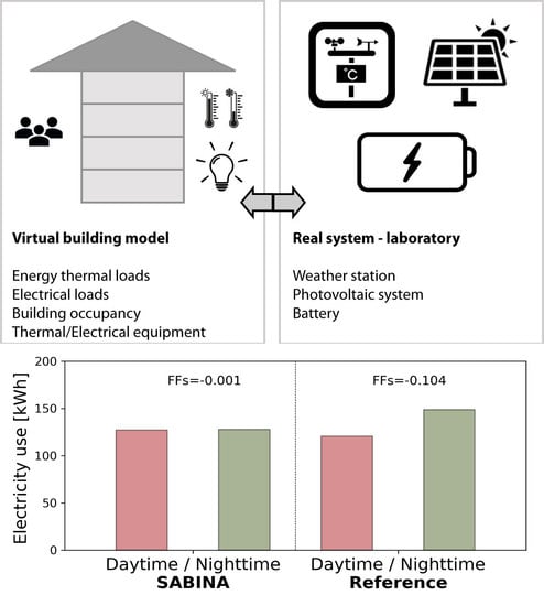
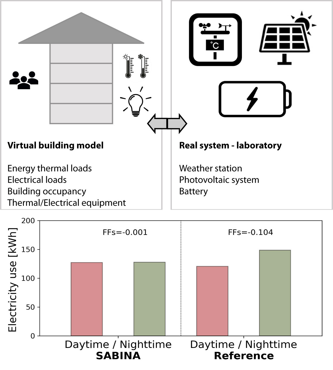
Figure 2 shows a general overview of the system, highlighting the real (weather info, photovoltaic generation and battery) and simulated elements (thermal and electricity loads, occupancy and other thermal and electrical equipment), and providing a representation of the building model geometry. The main objective of the building model is to simulate the components that are not present in the laboratory environment, as for example the building itself.

The building thermal behavior, the consumption of the non-real appliances and the real-time interaction are simulated through an EnergyPlus model wrapped in a Functional Mock-up Unit, similar to the configuration described in [11]. EnergyPlus has been selected since it is a very well known and open-access building simulation software. More details of how the model was built and calibrated is found in other publications [12,13] derived from the same SABINA project.

2.2. SmartLab Laboratory Environment

The Energy SmartLab test facility is composed of an electricity network that integrates a set of real devices that inject or withdraw energy to/from it. All devices include control hardware able to communicate with a centralized system that manages the electricity flows within the laboratory. More details about the facility can be found in Péan et al. [14]. Figure 3 shows the laboratory layout installed in order to manage both hardware and software subsystems for SABINA testing, including the SAFT Li-ion battery managed by a local controller board and the SCADA as a central node that supervises the measures and redirects the control actions coming from the EnergyPlus building model, the aggregator core and the battery. The main equipment used in the experimental setting is:

• Local Controllers: they are the communication interfaces between the power converter emulators and the SCADA in the laboratory. They read and write the necessary data directly from and to the cabinets via CAN, providing the data in a standardized register map in Modbus TCP.
• SCADA: it is the central monitoring node of the SmartLab laboratory. It supports the EnergyPlus and other modelling and simulation software.
• Internal broker: The SmartLab internal broker works as communication bridge between SCADA and the aggregator core.
• SAFT Li-ion battery and power converters: The 10 kWh lithium-ion battery used in SABINA tests charges and discharges directly on the grid side. It is connected to an AC/DC converter limited to 4 kW.

2.3. Building Algorithm

The building algorithm is the element in the system in charge of taking advantage of the intrinsic energy flexibility of a building to improve the building’s own performance. The BA is the first level algorithm that monitors and controls the state and set-points of the flexible elements within the building. The BA has four main objectives, which correspond to individual processes illustrated in Figure 4, where PID stands for process identifier:

• PID 1: Reading measurements from the broker (aggregator core) and writing them into a database to be used for the following processes to come.
• PID 2: responding to flexibility requests by the MIDA. This exchange can be initiated once per day by the MIDA.
• PID 3: computing a flexibility map that is provided to the District Algorithm. This operation is done on a daily basis.
• PID 4: computing the necessary set-points for the various technical systems at building level to enhance renewables penetration on the basis of model predictive control (MPC) optimization. This real time optimization runs every 15 min in order to compute the technical system set-points.

The core of the BA is the model predictive controller (MPC, also called optimization in PID 4), that has two main means of actions to fulfill its objectives:

• The building envelope can be used to store thermal energy, by performing overheating or cooling by using heat-pumps (HP), chillers, radiators or fan coils, for instance.
• The batteries (if available) can be employed to store electricity in a more direct way. These can be in house batteries (i.e., fixed) capable of charges and discharges.

In order to carry out the prediction needed for the optimization to take place, self-built models of the considered elements are generated. The BA uses an encoder-decoder architecture based on long-short term memory (LSTM) neural networks [15] to model the thermal aspects (i.e., building envelope, heat pumps, etc.), which are trained using the available EnergyPlus models. When available, real data is used to refine the models. The encoder-decoder architecture is well suited to model non-linear dynamic systems [16]. For the batteries, simple linear models with losses are employed. These models are included into an optimization problem that combines an objective function that minimizes the total energy exchanged from/to the grid (aiming at maximizing self-consumption), as well as constraints associated to heating, cooling and batteries. The optimization is performed for a horizon of 24 h discretized into H samples (H depending on the system sampling frequency).

The reduced model predicts the building state for the 24 h horizon considering the state of the building for the past 6 h and the forecasted PV power production. The algorithm counts on a virtual tariff or weighting function that controls the energy consumption and that is kept constant for the normal control. The interaction with the second level algorithm (MIDA) is found with two simple elements. One is the flexibility map, and the other is related to the activation of flexibility. 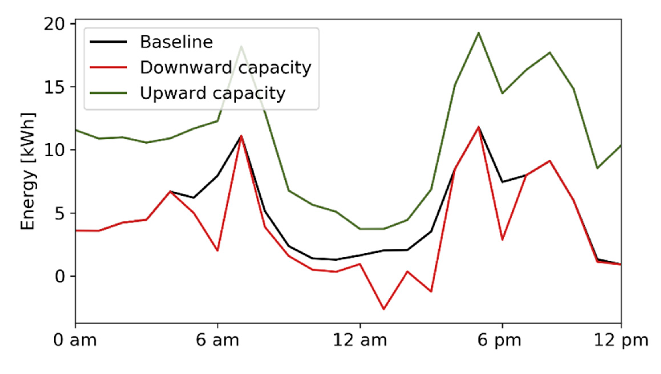The flexibility map, which corresponds to PID 3 in Figure 4, is computed once per day and refers to what the building expects to do and what it is capable to offer in terms of energy flexibility. Then, it computes the baseline (i.e., the expected consumption), the minimal (dDownward capacity) and maximal (upward capacity) energy that can be consumed for each hour, over a horizon of 24 h (an illustration of such flexibility map is provided in Figure 5). This computation involves solving 48 optimization problems in a receding fashion, with the same objective function as in the problem but with some slight changes. Based on the baseline profile, the flexibility map is computed by solving an MPC problem shifted over time to the corresponding activation hour ($q)$, i.e., the prediction horizon is $\left[q,q+24\right]$ and, with the virtual tariff $c\left(t\right)$ increased (upward capacity) or decreased (downward capacity) for the first hour in the prediction horizon. This process is repeated for the next 24 h to obtain the whole Flexibility Map. Once per day, this flexibility map is sent to the Market Integrated District Algorithm (MIDA).

This process is handled by the PID 2 of Figure 4. In order to compute the possible activation flexibility, the objective function of the MPC includes an additional soft constraint for the total energy during the first hour. The purpose of the additional soft constraint is to verify if the requested flexibility can be met, thus it constrains this amount of energy to be within the interval $\left[E_{min},E_{max}\right]$, where $E_{min}$ and $E_{max}$ are defined as follows. Let $E_{flex}$ be the flexibility requested by the MIDA and let $E_b$ be the expected baseline energy for the requested hour. If a positive activation is received (upwards, meaning to increase the consumption of the building) $E_{min}=E_b$ and $E_{max}=E_b+E_{flex}$. On the other hand, if a negative activation is received (downwards, meaning to decrease the consumption of the building) $E_{min}=E_b-E_{flex}$ and $E_{max}=E_b$. If the BA finds that it can provide the flexibility requested, then it will send a positive response to the MIDA. If not, the BA will send how much flexibility it can provide. If a final confirmation is received from the MIDA, the BA will apply the found solution. If not, the normal MPC is used to compute the control actions. This process is further explained in the following Section 2.4 regarding the flexibility activation by the MIDA.

2.4. Market Integrated District Algorithm

The goal of the MIDA is to participate into balancing markets by aggregating the energy flexibility from different buildings trying to reduce the ecological footprint of the electricity consumption while offering an economic incentive to the prosumer (building) for its participation in these flexibility services. The MIDA receives information from both the electricity market and from the BA. From the MI it receives the electricity (PVPC) and balancing market prices for energy and capacity. From the BA it receives information regarding the expected consumption for the next day and the expected flexibility upwards and downwards at every hour (the Flexibility Map described in Section 2.3). MIDA is a demand aggregator that counts on the information given by local energy management systems (BA in this case) to select the best moment to ask for flexibility to each building considering that only one activation per day with a duration of one hour is allowed per building in the framework of SABINA. MIDA follows a centralized strategy, meaning that it decides which building participates in any moment, in a similar way to what other research has proposed [17,18]. However, this is not the only option to aggregate demand response, literature has analyzed cooperative [19,20] and non-cooperative [21] decentralized strategies that may also work rather well. Nonetheless, centralized strategies generally provide much more knowledge of what would be likely to occur (as it goes by the hand of massive monitoring) and are best seen from a business low risk perspective.

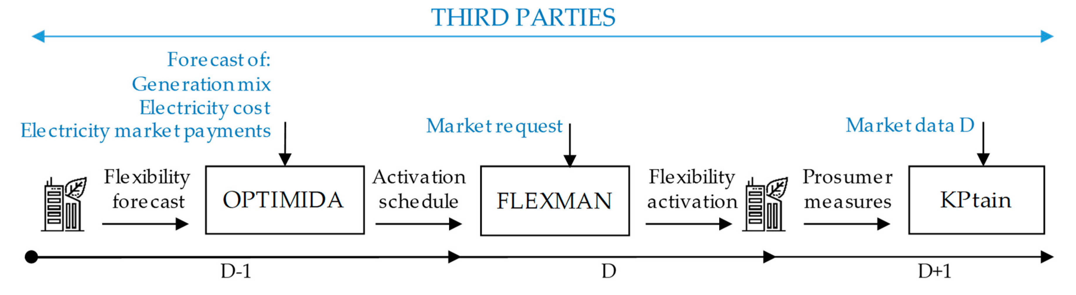
Note that, as described in Section 2.3, not all the elements in the building are capable to provide flexibility. In fact, the flexibility of the building is provided, in SABINA, by just a few elements. On one side, there are the thermally related elements that mainly consist in the envelope of the system that allows storing energy in its thermal mass. On the other side, there are the pure electric elements, such as PV panels, a community battery, and appliances among others, but only the battery is capable of changing its consumption pattern according to the BA decision. MIDA is developed in three modules based on the computation needs at different moments and the corresponding exchange of messages with the BA and the SABINA broker. These modules are the OPTIMIDA, the FLEXMAN and the KPtaIn:

• OPTIMIDA is the first module to act. During the day ahead it optimizes the activation of the available flexibility of all buildings in the neighborhood minimizing the CO₂ emissions taking the energy information available in the flexibility map of each building for the next day and the CO₂ emissions and tariffs from the market interface. To do so, Equation (1) is the mathematical expression that rules the module:

  $$f\left(DA\right)=Min {\displaystyle \sum }_{h=0}^{24}Emissions Fle{x}_h=$$

  $$=Min {\displaystyle \sum }_{h=0}^{24}{\displaystyle \sum }_{i=1}^n\left(\left({\beta }_{∆ih}·Fle{x}_{∆ih}·Mi{x}_h\right)-{\displaystyle \sum }_r\left(Bas{e}_{∆ihr}-Re{b}_{∆ihr}\right)Mi{x}_{hr} \right)$$

  (1)

  $$-\left(\left({\beta }_{\nabla ih}·Fle{x}_{\nabla ih}·Mi{x}_h\right)- {\displaystyle \sum }_r\left(Bas{e}_{\nabla ihr}-Re{b}_{\nabla ihr}\right)Mi{x}_{hr}\right)$$

where $Fle{x}_{∆ih}$ is the available flexibility of a building (i) at a certain hour of activation (h) and the $∆or\nabla$ refers to the direction of the flexibility, that is, to increase or decrease the consumption of the building. ${\beta }_{∆ih}$ is a parameter between 0 and 1 that indicates how much of the total available flexibility should be used. 0 means no activation and 1 asks for the whole capacity of the building for the corresponding hour. The module considers activations upwards and downwards (first and second brackets) and not only the effect of the activation (first sub-brackets) but also of the corresponding expected rebound effect (second sub-brackets). To compute the emissions caused by the rebound effect, the equation considers the expected baseline curve ($Bas{e}_{∆ihr}$) and subtracts the amount of energy corresponding to the “new” baseline derived from the activation of flexibility ($Re{b}_{∆ihr}$) for the amount of time of the rebound effect (r). In all cases, the energy shifted is multiplied by the corresponding electricity emissions mix for each hour ($Mi{x}_{h}andMi{x}_{hr}$).

The activation of district flexibility should not carry any economic penalty for the owners of the buildings. Therefore, several restrictions should be respected:

$$V_{capDA}+V_{flex∆DA}-C_{∆\mathrm{DA}}\ge 0.$$

(2)

$$V_{capDA}+V_{flex\nabla DA}-{\mathrm{C}}_{\nabla \mathrm{DA}}\ge 0.$$

(3)

Equations (2) and (3) express these economic restrictions, indicating that the added value from capacity ($V_{\mathrm{capDA}}$) and use of energy (${\mathrm{V}}_{\mathrm{flex}∆\mathrm{DA}}$) payments should always be higher than the energy costs derived from the activation ($C_{∆DA}$) that, as it occurs with Equation (1), considers also the rebound effect in the same way but using the price of electricity (PVPC) instead of the electricity mix.

Additionally, there are several combined binary restrictions to ensure the correct performance of the whole activation system. That is, to ensure that only one activation is done per day, that the activation does not occur within the rebound effect of the previous activation and to limit the duration of the flexibility activation to one hour.

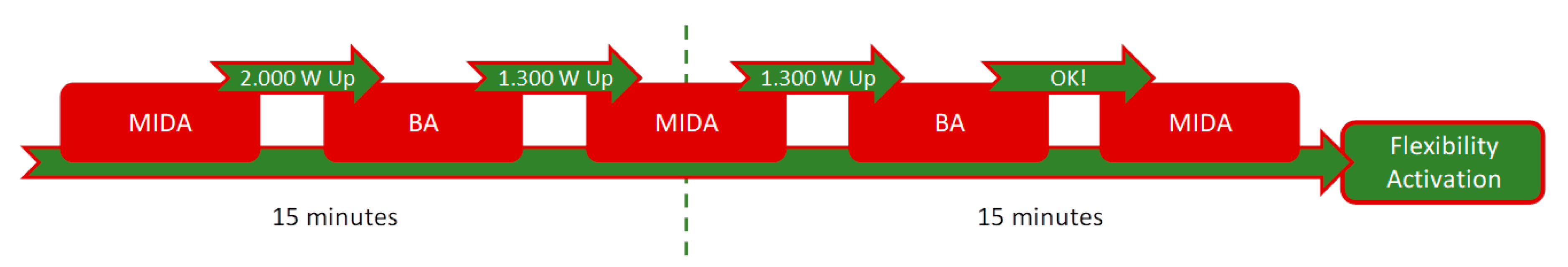
• FLEXMAN acts during the day in real-time. Whenever an activation of flexibility is required by the electricity grid (which is generally lower than what was offered), FLEXMAN first confirms the flexibility availability of each building (BA). After receiving a response from the building (see the BA process at the end of Section 2.3) MIDA re-computes the allocation of flexibility with the rest of buildings in its portfolio. Then, it proceeds to confirm (or not) the activation of each building by indicating the amount of energy required to the BA. Note that it will never ask for more energy than what the BA had previously indicated. An illustration of the process is presented in Figure 6.
• KPtaIn module is the last one to act. It is in charge of evaluating the effectiveness of the activation by analyzing the Key Performance Indicators (KPIs), so its activation occurs during the day after. Final costs and environmental factors of the activation of flexibility are calculated and published in the broker. The KPIs are described in Section 2.6. Figure 7 presents a visual representation of the modular configuration of MIDA described.

Note that, in no case, does MIDA take control or interfere with what the BA does, relying on the goodness of its forecasts and performance, similarly to what Iria et al. proposed [23], but in our case, all the BA are cloud connected, meaning that the machines in the buildings that activate the elements within are really simple and affordable while all the calculations are done by the MPC in the cloud. This approach reduces the initial investment by the owners, which might incentivize their willing to install such elements. The only way it has to improve the quality of the aggregated energy provided for balancing services is to evaluate each building through a performance index, calling more often those buildings that perform better and excluding those that are less accurate or reliable. This is not the only way to proceed as aggregator, some research proposes to go deeper into the houses and take control of each element as done in [24,25]. In SABINA, the services of energy efficiency (BA) and demand response (MIDA) are done by two different elements (that could, for instance, be different companies). In studies such as the ones just mentioned that go directly to control the active element, this situation is rare as it would mean that two different companies may act on the same element.

Finally, although MIDA acts on a global way considering many buildings (simulated in the project), this study presents only the results from the activations of one building (the one simulated and emulated through SmartLab) to clearly identify the benefits it represents individually. Considering that all the elements in explained in the study refer to a single building, it was considered that mixing both approaches might confuse the reader.

2.5. KPI for Evaluating Thermal Comfort

The thermal sensation of the body can be predicted with the Predicted Mean Vote (PMV) and the Predicted Percentage of Dissatisfied (PPD), which represents the discomfort or dissatisfaction based on estimating the percentage of people susceptible to feeling too hot or cold. Both indices are based on the Fanger model that is valid for buildings with active heating and cooling systems. These parameters can be classified into three categories of thermal comfort, depending on the requirement of the building.

Table 1. Thermal environment categories.

Category	PPD %	PMV	Explanation
I	< 6	−0.2 < PMV < 0.2	High standard, recommended for spaces occupied by people with special requirements.
II	< 10	−0.5 < PMV <0.5	Normal level of requirement; It should be used for new and renovated buildings.
III	< 15	−0.7 < PMV < 0.7	Acceptable/moderate level of requirement; can be used in existing buildings.
IV	> 16	PMV < −0.7 and PMV > 0.7	Values outside the criteria of the previous categories. This category should only be accepted during a limited part of the year.

defines the thermal environment categories [26]. The KPI used to assess the level of thermal comfort is the percentage of time that the occupants are in the defined categories.

2.6. KPIs for Evaluating Flexibility

Energy shift flexibility factor (FF_S) is an indicator that measures the capability for shifting the energy consumption between periods [27]. In SABINA, the optimization aims to shift the energy consumption toward sunlight hours in order to maximize the use of on-site renewables (photovoltaic). For this reason, Equation (4) represents the formulation of the FF_S for this case, where l(t) is the building electrical load:

$$F{F}_S= \frac{{\int }_{DT}^{ }l\left(t\right) dt-{\int }_{NT}^{ }l\left(t\right) dt }{{\int }_{DT}^{ }l\left(t\right) dt+{\int }_{NT}^{ }l\left(t\right) dt}$$

(4)

FF_S = 1 means that all the energy consumption occurs during daytime (DT) hours; while FF_S = −1 represents the opposite, that all consumption occurs during nighttime (NT). A FF_S = 0 means that the total amount of energy consumed during day and night is the same.

Regarding energy savings, the KPI corresponds to Equation (5), where savings are calculated by the subtract of the consumption for the reference scenario P_ref(t) to the real consumption of the building P(t). Note that this value may be negative if no improvement is observed. In this case there will be energy losses instead of savings:

$$Energy Savings = \underset{0}{\overset{24}{{\displaystyle \int }}}P\left(t\right)-P_{ref}\left(t\right) dt.$$

(5)

Multiplying the difference between the reference and SABINA’s consumption by the emissions’ mix of the electricity that comes from the grid it is easy to obtain the environmental savings (Equation (6)):

$$Environmental Savings = \underset{0}{\overset{24}{{\displaystyle \int }}}\left(P\left(t\right)-P_{Ref}\left(t\right)\right)\ast Mix\left(t\right)dt.$$

(6)

To calculate the economic savings, in addition to multiplying for the electricity price (PVPC), it is needed to add the earnings that come from the balancing market, as described in Equation (7):

$$Cost Savings=E_{Flex}·{€}_{use}+E_{FlexMap}·{€}_{cap}+\underset{0}{\overset{24}{{\displaystyle \int }}}\left(P\left(t\right)-P_{ref}\left(t\right)\right)·PVPC\left(t\right)dt.$$

(7)

where E_Flex $\cdots$ €_use correspond to the energy use and E_FlexMap $\cdots$ €_Cap to the capacity payments considering the Flexibility offered by the building in the day ahead Flexibility Map.

3. Results and Discussion

The experiment comprises two scenarios that last for two days and uses real recorded data from March 5th to March 6th. The experiment proved the technical feasibility of the proposed configuration and the correct implementation of the entire communication chain between the algorithms, models and real equipment.

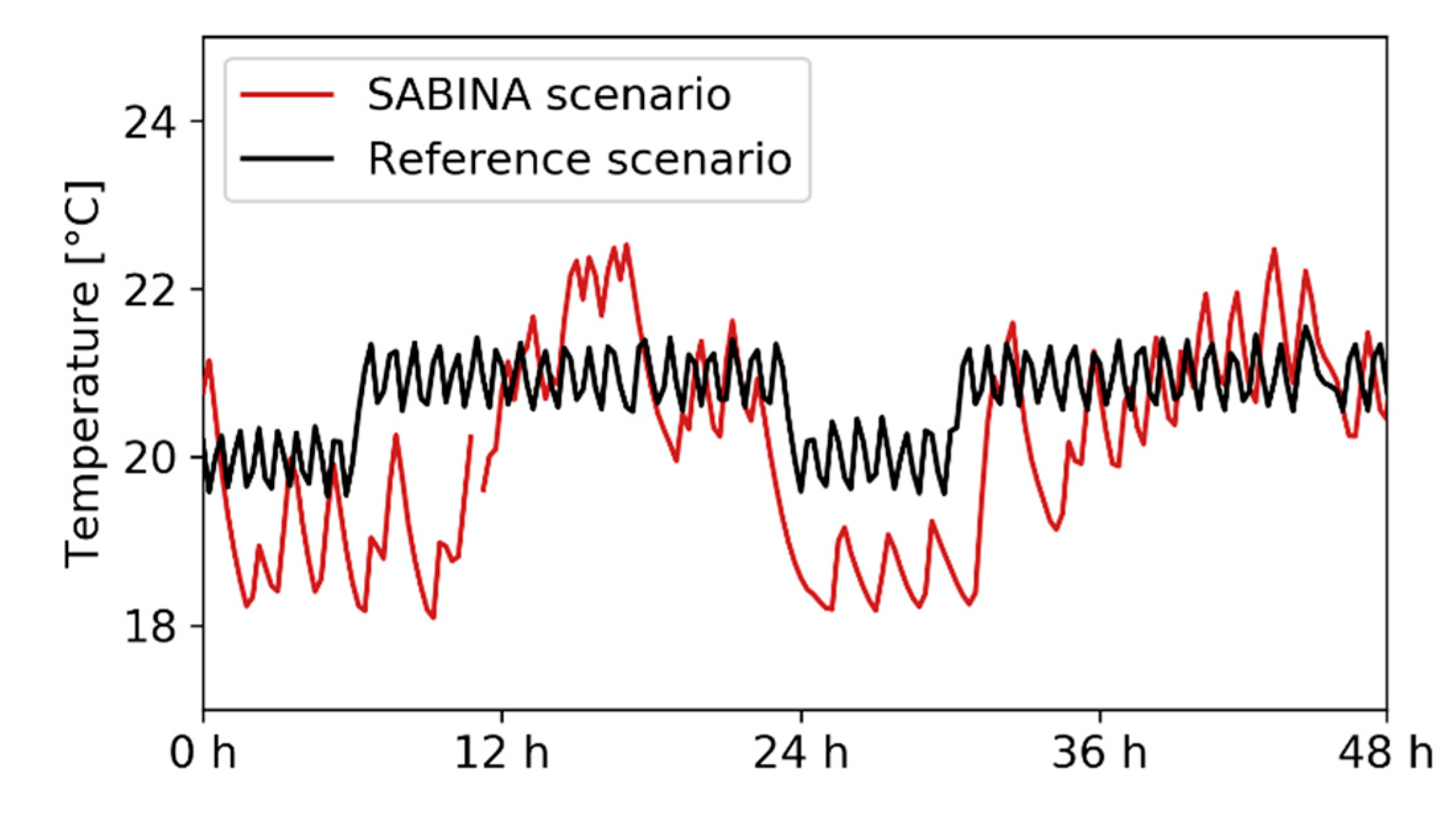
Figure 8 shows the average temperature between day and night zones of the ground floor dwelling. On the left axis it is reported the thermal comfort range in which the BA could operate meanwhile on the bottom axis are reported the hours of experiment. Notice that temperatures in the reference scenario (black curve) follows the fixed setpoints assigned. They are set to 20.5 °C from 0 h to 6 h and from 23 h to 00 h that are considered sleeping hours, while the rest of the hours are considered active ones. During active hours, temperature setpoints are fixed to 21.5 °C. On the other hand, SABINA’s temperatures range from 18 °C to 23 °C following the setpoints received from the BA.

This change in the thermal load is correlated with the day/night hours shifting strategy of the BA. During late daylight hours it increases the consumption to pre-heat the building while, at night, when people is sleeping and covered with thick blankets, temperature is visibly reduced. Note that, for the second day, there is not much pre-heating, as not much PV generation was forecasted and day/night consumption shifting was less relevant.

This temperature change has an impact on thermal comfort, Figure 9 shows the percentage of time in which thermal comfort lays in each comfort category. The evaluation has been done averaging the PPD of the different dwellings and excluding time without occupancy. It can be noticed (considering night time: 2.5 clothes resistance, activity 0.8 Met; daytime 1 clothes resistance, activity 1.2 Met [28]) that the temperature variations observed in SABINA solution do not jeopardize comfort in a critical way. Indeed, almost the 90% of the time, comfort level lies in category II that corresponds to a normal level of requirement. This is mainly due to the presence of “comfort” constraints in the mathematical formulation of the BA that limits the set of feasible solutions. It is mostly through increasing the share of time in which people stays in category II (still in good comfort) that the BA achieves energy savings from night consumption.

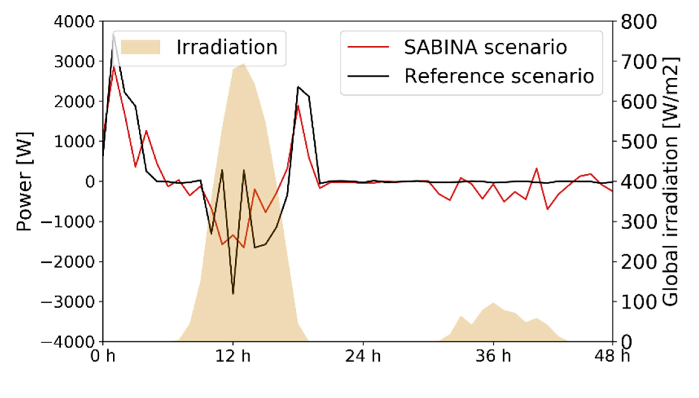
Regarding the real electric equipment, which is the 10 kWh community battery, Figure 10 presents the charge/discharge profiles observed during the test (on the left axis) and the global irradiance measured at the weather station. Note that the second day corresponds to a cloudy winter day with low irradiation and, consequently, with almost no PV production. The maximum charge/discharge power supported by the power converters is 4000 W and it is reported on the left axis.

Reference scenario profile (black curve) follows a typical “self-consumption” behavior programmed with a conditional statement. Indeed, the battery stores energy during sunlight hours if the photovoltaic production is greater than the building electrical demand and it gives the energy back during nighttime. SABINA scenario profile, instead, follows the setpoints received from the BA that tries to enhance the on-site consumption. Note that there is not much “conceptual” difference in the use of the battery by the MPC in SABINA and the simple conditioned algorithm of the battery in the reference scenario, although SABINA uses slightly less the battery. This is because both systems pursue the same goal of maximizing self-consumption. Relating Figure 8 with Figure 10, which refers to the thermal and electric storage capacities of the building, it is relevant to notice that the BA decides to store more energy using the thermal mass of the building (overheating strategy during sunlight hours) rather than using the community battery.

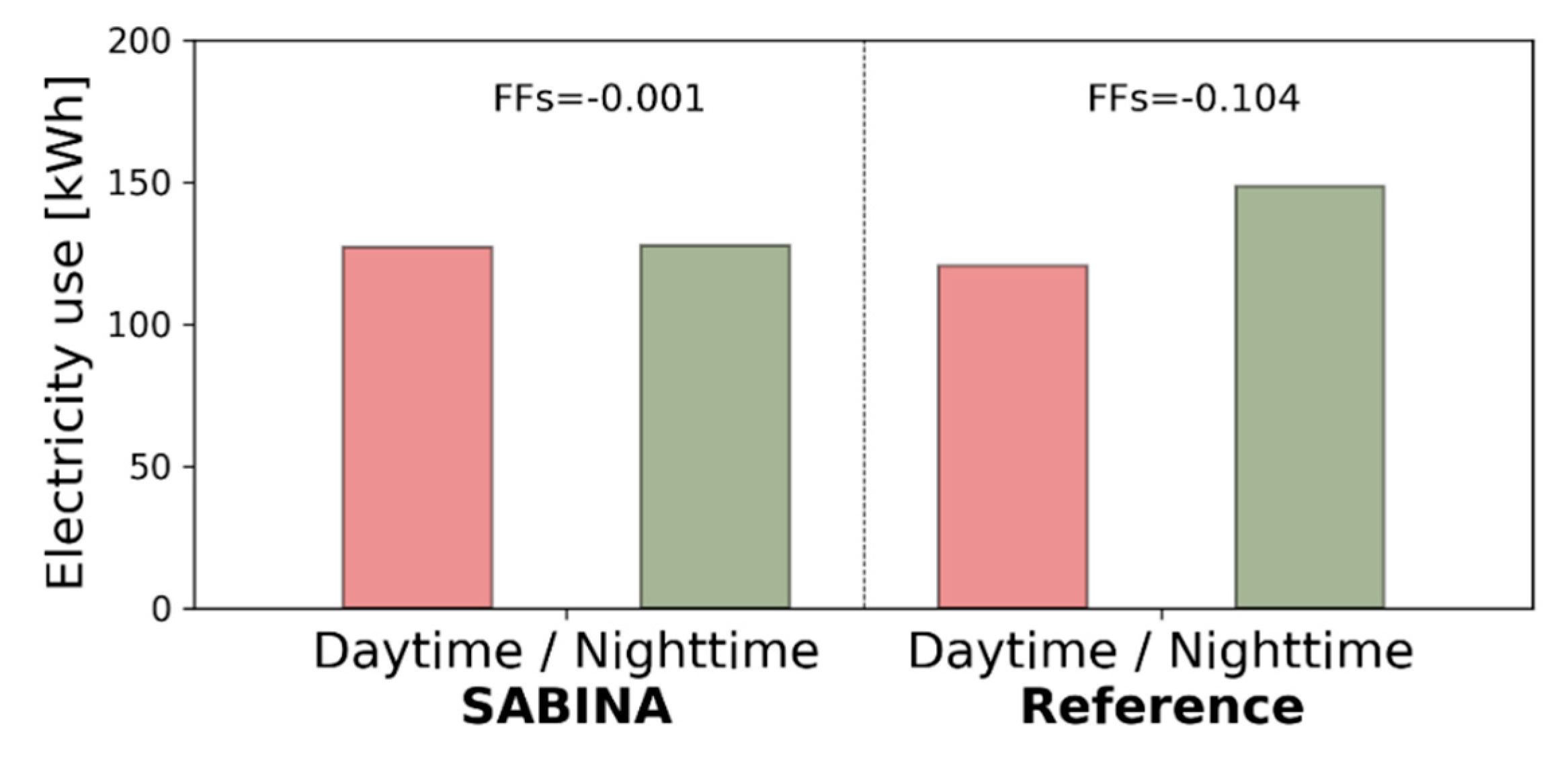
In order to assess the advantages of the BA and the achieved performance, Figure 11 compares SABINA and reference scenario in terms of energy consumption (left axis) Red bars represent the building energy consumption during daytime while green bars represent the nighttime consumption.

SABINA solution successes to reduce the energy demand and, more important since it is the objective of the BA, it achieves a relevant energy shift from night hours to daylight hours. Recall that, as mentioned in the introduction, the main goal of the BA is to maximize self-consumption, which could be also understood as minimizing the energy exports caused by the excess of PV generation. Thus, consuming more energy during daylight hours allows consuming in situ the energy produced by the photovoltaic panels and reduce exports. However, the energy exported in the reference scenario, see

Table 2. Electrical balance comparison.

Scenario	Imported (kWh)	Exported (kWh)	Demand (kWh)	PV (kWh)	Battery Charge (kWh)	Battery Discharge (kWh)
Reference	206.8	5.1	256.7	50.8	15.3	19.5
SABINA	187.3	1.0	237.5	50.8	17.3	17.7

, is limited and corresponds, mainly, to the first day, having not much margin to obtain additional benefits by increasing even more the consumption during daylight hours. The fact that results in consumption for day and night hours are so similar in the case of SABINA is just a coincidence from the analyzed case, results slightly vary from day to day analysis.

The quite high consumption of both scenarios is mainly due to the four heat pumps that consume about 16 kWh per day to provide SH and DHW. The rest of the energy consumption accounts for appliances, lighting needs and auxiliary equipment presents in the system. Figure 12 represents with a Sankey chart the energy flows of the system.

Table 2 summarizes the electrical balances of both scenarios where the sum of imported energy, PV production and battery discharge are equal to the sum of the exported energy and the electrical demand. Notice that, in the SABINA solution, the energy exported to the grid is almost four times lower than the reference scenario.

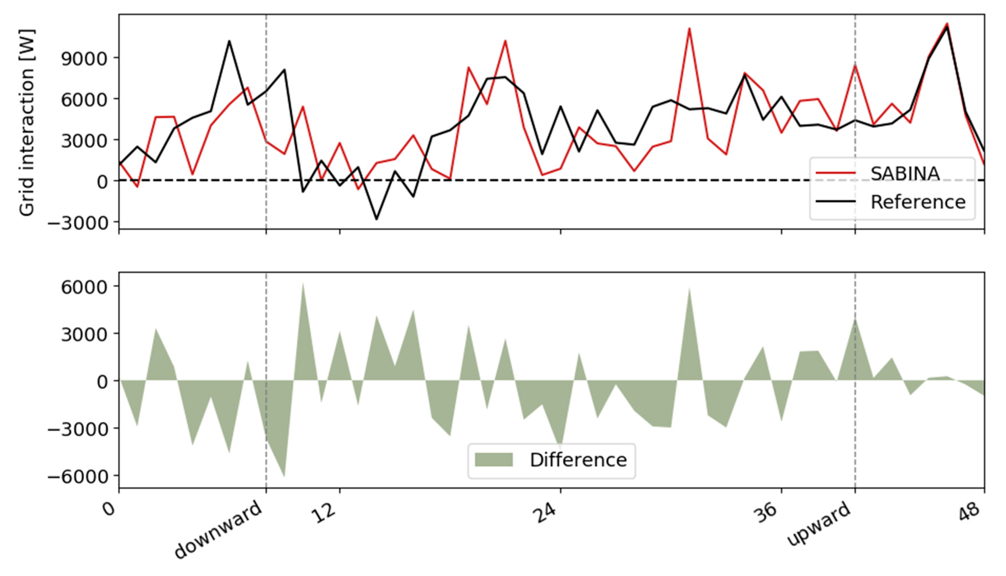
Grid interaction can be better explained referring to Figure 13. The top subplot shows the grid interaction of SABINA solution in red and the reference one in black. Negative values represent the power injected to the grid while positive ones represent the power imported. The plot shows in a direct way the goodness of the BA which minimizes the energy exportation during mid-day hours.

In addition, Figure 13 marks the flexibility activations at the respective moments and direction. Notice also that the low irradiation of the second day implies no energy exports in any of the scenarios and this is also a factor that significantly affects the capacity of SABINA to reduce energy consumption.

In the bottom subplot, the green area highlights the energy shift between SABINA and reference scenario per hour. This representation is useful to detect the upward and downward capability in terms of energy shift of the SABINA scenario compared to the reference one and visualizes the consumption increase during daylight hours and the major reduction that occurs during night hours.

The flexibility activations from the balancing markets take place at two moments. At 8 h in the morning the first day there’s a downwards activation and at 16 h during the second day the activation is upwards.

Table 3. Flexibility activation results.

Day	Activation Hour	Energy Flexibility Map (Wh)	Energy Confirmation (Wh)	Energy Delivered (Wh)
05/03/2019	8	−5939	−3090.79	−2169.01
06/03/2019	16	6162.79	6534.01	5635.33

presents the overall results.

Table 3 presents the differences in the amount of energy indicated by the BA in the Flexibility Map and what the BA finally confirms that the building should be capable to provide when the flexibility is requested. Similarly, the effective energy delivered slightly differs to what it was just confirmed before the activation. The explanation to these variation is found in the stochastic events of what people in the building might do in comparison to what the BA expected them to do. Note that, apart from the first activation (which is computed taking warm-up data as it is the beginning of the experiment and estimations are less robust) the second activation has a closer result to what the MIDA asked for, meaning that the BA projections during the day ahead are sufficiently accurate.

Note also that the activation of MIDA follows the minimization of emissions, which could be related (but not entirely correlated) to the reduction of consumption and might interfere with the main objective of the BA. In fact,

Table 4. Flexibility results.

Day	Case	Energy (kWh)	Cost (€)	Emissions (CO2)	Primary Energy (Wh)
5/03/2019	SABINA	75,625.59	7.35	9.37	155,639.34
	REFERENCE	81,295.26	8.42	10.22	174,802.11
	SAVINGS	−5669.68	−1.08	−0.85	-19,162.78
	SAVINGS (%)	−7%	−13%	−8%	−11%
6/03/2019	SABINA	114,470.70	12.42	31.78	270,829.58
	REFERENCE	119,929.92	13.39	33.65	284,568.21
	SAVINGS	−5459.22	−0.97	−1.87	−13,738.63
	SAVINGS (%)	−5%	−7%	−6%	−5%

shows that, whenever there is a reduction in the consumption of the building, the emissions and costs savings are slightly higher than the corresponding reduction in the energy consumption. These higher shares in savings mean that, effectively, the use of MIDA in SABINA incentivizes the use of energy when it is less pollutant and reverts in an increase of the economic savings thanks to the revenues obtained by the market participation. In fact, the direct payments from the electricity markets correspond, in its majority, to capacity payments and in a less determinant way through delivery payments, which account for 0.49€ and 0.38€ savings. The slight differences in revenues from market participation are basically caused by the amount of energy offered during the day ahead taken from the flexibility map. However, the share is drastically reduced when comparing the first and second day. This lower overall impact is caused by the fact that, having no PV generation to use in the second day, the building has no other alternative than to buy energy to the electricity grid to cover what the PV “normally” does in a sunny day and the final cost increase to cover the energy demand of the building turns to be substantially higher. Thus, although the revenues from market participation are similar in absolute values, they double in relative terms.

To understand the results of Table 4, please consider that savings are presented with a negative sign.

In this same direction, Table 4 shows in the last column, the changes in the primary energy consumption. Primary energy refers to the amount of energy needed to generate the energy consumed by the building as final user considering all the losses upstream such as extraction of raw materials (fuel), transportation (of the source or energy) or combustion. Although in both days the value of primary energy savings in Wh is higher than the energy savings from the building (basically caused by the factor higher than 2 that accompanies fuel based power sources [29]), only for the first day the share of saving is higher in the first day while it is maintained for the second day. The reason behind this significant difference is, basically, that there is an increase on PV self-consumption during the first day (or a reduction of the exported energy that has to be later imported with worse primary energy values) which does not occur on the second day due to the lack of sunlight.

4. Conclusions

This study shows that the semi-virtual laboratory testing is useful to test flexibility capacities from buildings prior to full deployment in the market. The implementation of SABINA with a two level optimization process was successfully achieved in the laboratory environment. One of the limitations of this study is that results are partially simulated. Moreover, it has to be remarked that EnergyPlus is not the most suitable simulation software to perform hardware in loop simulations due to its limited co-simulations options available. Nonetheless, SABINA is now being installed in two real buildings from the technological and cultural park in Lavrion (Greece) and in two schools in Denmark to evaluate the possibilities of the solution in real environments.

This laboratory tests validated that, in the first place, there is a reduction of the electricity injected to the grid. This fact is supported by the increase of self-consumption, i.e., almost all the electricity generated by the solar panels in the building is consumed by the same building. Additionally, results show that there is a shift of energy consumption towards daylight hours, when there is more generation of energy and, thus, when an increase of the consumption is aligned with the objective of the building algorithm to maximize the load cover factor. Results also highlight the high impact of solar energy production in the capacity of the system to improve the consumption behavior of the building, that is, in cloudy days, the goodness of the solution is not as good as in sunny days. Moreover, the building algorithm correctly forecasts the availability of extrinsic flexibility to the MIDA, which is a non-trivial resolution, as stochastic events from people entering and leaving the households clearly deviate the energy consumption of the building against what the BA expected during the day ahead forecast.

In general terms, the reduction of emissions and cost is higher than the sole reduction of energy consumption. This implies that, effectively, flexibility activations are reasonably used, considering that the main driver of MIDA is the reduction of greenhouse gas emissions. Note also that, in relative terms, the cost benefits are even higher than the environmental ones even though MIDA’s main goal was environmentally driven. This higher impact is caused by the additional payments from the service given to the distribution or transmission system operator, when these payments are not taken into consideration, savings are similar in both categories.

These positive results are obtained from a two-winter-day test in one building. However, differences in buildings thermal mass, end users’ operation, controllable electrical equipment and weather (season of the year) might affect in a relevant way to SABINA’s potential results. For instance, when there is less heating demand and no electric storage devices, it will be harder to obtain this energy consumption shift from night to day.

This semi-virtual test confirm that the energy flexibility of buildings is possible and that they are capable to react within a 15 min’ range and for one hour of duration using the thermal mass of buildings. This concept might be interesting for new demand aggregators’ business to consider.