Application of Rough Set Theory (RST) to Forecast Energy Consumption in Buildings Undergoing Thermal Modernization


Faculty of Production and Power Engineering, University of Agriculture in Krakow, 30-149 Kraków, Poland
*
Author to whom correspondence should be addressed.
Energies 2020, 13(6), 1309; https://0-doi-org.brum.beds.ac.uk/10.3390/en13061309
Submission received: 8 February 2020
/
Revised: 26 February 2020
/
Accepted: 7 March 2020
/
Published: 11 March 2020
(This article belongs to the Special Issue Evaluation of Energy Efficiency and Flexibility in Smart Buildings)
Abstract
:In many regions, the heat used for space heating is a basic item in the energy balance of a building and significantly affects its operating costs. The accuracy of the assessment of heat consumption in an existing building and the determination of the main components of heat loss depends to a large extent on whether the energy efficiency improvement targets set in the thermal upgrading project are achieved. A frequent problem in the case of energy calculations is the lack of complete architectural and construction documentation of the analyzed objects. Therefore, there is a need to search for methods that will be suitable for a quick technical analysis of measures taken to improve energy efficiency in existing buildings. These methods should have satisfactory results in predicting energy consumption where the input is limited, inaccurate, or uncertain. Therefore, the aim of this work was to test the usefulness of a model based on Rough Set Theory (RST) for estimating the thermal energy consumption of buildings undergoing an energy renovation. The research was carried out on a group of 109 thermally improved residential buildings, for which energy performance was based on actual energy consumption before and after thermal modernization. Specific sets of important variables characterizing the examined buildings were distinguished. The groups of variables were used to estimate energy consumption in such a way as to obtain a compromise between the effort of obtaining them and the quality of the forecast. This has allowed the construction of a prediction model that allows the use of a fast, relatively simple procedure to estimate the final energy demand rate for heating buildings.
1. Introduction
In the climatic conditions of central and eastern Europe, the heat used to heat rooms is a basic item in the building’s energy balance and significantly affects its operating costs. The accuracy of the assessment of heat consumption in an existing building and identification of the main components of heat loss depends largely on whether the energy and economic effects assumed in the thermal modernization project are achieved.
Activities aimed at improving the thermal efficiency of buildings, and thus affecting the thermal comfort of users, usually consist in increasing their energy standard. In the case of buildings that existed before taking action to save energy, there is a need to prepare an energy audit, the purpose of which is to obtain adequate knowledge of the existing energy consumption profile of a given building or buildings complex, determine the manner and amount of energy that can be obtained, and notify about the results.
The objective of the audit is to determine the amount and structure of consumed energy and to identify and then recommend specific solutions that are energy profitable. The audit may identify modernization operations that are profitable in the investigated building and which products and technical solutions are the most favourable. Since 1999, there has been a program in Poland that supports actions aiming at reduction of energy consumption in existing buildings. It is set forth in the act on supporting thermal efficiency improvement and renovations [1], which is in line with the provisions of the EU Directive on the energy performance of buildings [2]. As a part of this program, a majority of apartment buildings are modernized—according to BGK [3], approximately 41,000 buildings were modernized. According to the statutory provisions, the auditing of buildings is based on the following stages: analysis of the present condition of buildings, verification of the assumed parameters based on the data on the real energy consumption, identification of possible facilitation along with determination of costs of their realization, calculation of savings resulting from facilitations (at the assumption that modernized partitions should have heat transmission ratios U lower or equal to the border values set forth in binding industry resolutions) and economic analysis of profitability, where it is assumed that investment expenditures incurred for a given facilitation should be returned within 10 years. Energy calculations in audits are made with a balance method (monthly or annual), where the auditor used the so-called diagnostic method that consists of estimation of parameter values. Current energy consumption is determined on this basis. When estimating energy consumption after thermal efficiency improvement, additionally economic aspects of the suggested energy saving solutions are included. This method is faulty due to the possibility of its use, which enables forecasting thermal energy consumption of single buildings. For the estimation of energy consumption for a bigger group of buildings, this method is too time consuming and requires a considerable work input.
Thus, it is necessary to look for other methods that will be suitable for analysis of the adopted thermal modernization measures and determine their impact on future heat consumption in existing buildings.
There are many methods to forecast current and future energy needs of buildings, which can be divided into three main groups [4,5,6]:
Engineering methods determine the thermal balance of the building, taking into account the use and efficiency of the heating/cooling and hot water preparation system. These models are used to determine the energy performance as well as to create forecasts of thermal comfort in buildings (user comfort). They are also used to determine indoor environment quality indicators. These models can be divided into two groups: dynamic and static. The dynamic models are based on the guidelines contained in EN 15251 [17], which defines the indoor environment conditions for individual rooms (thermal conditions for winter, thermal conditions for summer, air quality, criteria for ventilation, lighting and acoustics). They also take into account the influence of changing external conditions such as temperature, solar radiation intensity, wind speed, and others. They are mainly used in newly constructed (highly efficient) energy-saving and passive buildings [18,19,20]. Dynamic methods, determining the heat balance in short periods (usually 1 h), allow for a more accurate consideration of the effects related to the storage of heat or cold energy in the building’s structural elements. Static models are based on the European standard EN 13790 [21], which is also supplemented by the EN 12831 standard [22]. Based on this method, heat balance is determined for a long calculation period (usually one month or heating season). Such models can be found in the literature [23,24,25]. This method is also used when preparing energy audits. Statistical methods are mainly regression models that correlate energy consumption or energy index with independent variables, which can be either quantitative or qualitative. Empirical models are constructed on the basis of historical results, which means that before training the model, we have to collect enough historical data to achieve sufficient precision. Statistical regressions have been widely used both for research at the design stage and after—during the use of the building. Regression models are used to forecast energy consumption based on detailed data, such as the age of the building and its main geometrical and thermo-humidity parameters, such as for example: shape factor, area of the opaque and glazed partitions, heat transfer coefficient, and indoor and outdoor temperatures, etc. Model calculations were carried out in analyses of heat consumption in systems supplying entire housing estates or towns, as well as at the level of a single building [9,26]. In some simplified models, regression is used to correlate energy consumption with climatic variables (e.g., a degree-days) in order to obtain the energy performance index [4,5,27,28,29,30,31,32,33,34,35,36,37,38]. Although the simplicity of regression is generally an advantage of these models, it is also a disadvantage because most regression techniques cannot deal with non-linear phenomena that occur during the use of a building. In models based on artificial intelligence, artificial neural networks and their derivatives are most often used. This type of models is based on solving non-linear problems and is an effective approach to this complex issue. The detailed division of methods and input variables for modelling is discussed in the paper [4]. These are: weather data grouping all data related to outdoor conditions, indoor environment in the building (temperature, humidity, etc.); occupancy and behaviour of occupants; time indicators that provide information about the functioning of the building and its energy behavior; past time steps, which take into account the potential impact of past events on current and projected energy demand states of the building; and building characteristics with information about active and passive systems. In recent years, artificial neural networks have been used to analyse the energy consumption of different types of buildings for different processes, such as heating/cooling, electricity consumption, heat loss through partitions and optimisation of energy consumption and estimation of performance parameters. The use of artificial neural networks and machine learning methods for modelling energy consumption can be found in the works of many authors [9,39,40,41,42,43]. Most of the presented calculation methods can be successfully used to estimate energy consumption for heating/cooling and hot water preparation and to determine the energy performance for different thermal parameters of partitions, the way buildings are used, and weather variables [4,5]. The authors of these works mainly focus on energy modelling in buildings such as offices, hotels, schools, universities, etc. However, few works concern single and multi-family residential buildings. In particular, there is a lack of studies on real buildings [4], data for which are difficult to obtain. Individual energy demand in residential buildings is more difficult to estimate due to the lack of data on occupancy of buildings and the complexity of the inhabitants’ behaviour. Forecasting models focus mainly on estimating energy consumption, thermal comfort in existing (or simulated), newly built, energy efficient and passive facilities, for which it is possible to obtain reliable data on the insulation of building partitions, ventilation air streams, and number of inhabitants [18,19,20,44]. Most of the calculation methods presented are successfully suited for the estimation of energy consumption when determining the energy efficiency of buildings, for different parameters of thermal barriers, use, and variable weather conditions. Nevertheless, it is necessary to look for other solutions that could be used in the case of real buildings characterized by different availability of data describing the object from the thermal and operational point of view [14]. Another extremely important aspect of assessing energy consumption is the fact that the use of residential buildings often differs from the intended project. This is often due to the fact that the auditor’s calculations are in many cases based on unreliable and inaccurate data, which significantly affects the accuracy of the assessment of current and future energy consumption of a building. At each stage of the audit calculations, some characteristics are likely to be inaccurately estimated, most often the physical parameters of buildings and the way the building is used, due to the difficulty of collecting all the figures that characterize the building and its surroundings with sufficient precision. This applies in particular to the value of heat transfer coefficient U through the building envelope. In such cases, the auditor carries out the examination of partitions and then assesses the equivalent thermal resistance of the partition. Even methodologically correctly calculated resistances can be wrong, as it is necessary to determine the thermal conductivity and thickness of individual layers, which is not always possible. A frequent problem in thermal calculations is the lack of complete architectural and construction documentation of the analyzed objects. In addition, there are other factors that affect the accuracy of the calculations, which are due to e.g., moisture, ageing of the material, etc. Uncertainty as to the correct assessment of the heat transfer coefficient, as well as other important parameters, such as the volume of ventilation air flow, influences the result of the final assessment of heat demand for both the existing buildings and the buildings for which thermal modernization measures are planned. It is therefore advisable to test new methods that could be used for a rapid technical analysis of measures taken to improve energy efficiency and to determine their impact on future heat consumption in existing buildings. These tools should allow decision-makers to assess the potential for real energy savings resulting from planned actions to improve the thermal performance of buildings. One of these methods may be the Rough Set Theory (RST) method [45], which is developed to analyze inaccurate, generic and undefined data. The more so because this method—according to the literature review—has not been used so far in forecasting energy consumption in buildings [4,8,15,43]. Therefore, the aim of the research was to determine the usefulness of a model based on RST for estimating thermal energy consumption in buildings undergoing thermal improvement. Due to the different availability and accuracy of data describing the building, the used input variable configurations will be tested during model construction in such a way as to achieve a compromise between the effort of the auditor to obtain them and the quality of the forecast.
2. Materials and Methods
Before the main objective of the study was achieved, analyses were carried out to establish a potential list of explanatory variables (conditional attributes). During the research, a database was created covering 109 buildings from the end of the last century that were thermal improved in the years 2010–2015. These buildings had energy audits prepared, on the basis of which the optimum variants of thermal modernization were selected, the partitions that should be modernized were indicated, and the appropriate thicknesses of layers of thermal insulation materials were selected. The analyzed buildings were described with many parameters.
For experimental reasons, most relevant characteristics have been selected. Some of them are measured and others calculated, as pointed out in Table 1.
The average value of parameters describing the examined buildings is comparable to the data contained in the building typology “TABULA” for Poland. These parameters are typical for an “average building” of a multi-family residential building built in 1967–1985 [46,47]. Therefore, the surveyed group of buildings can be considered as representative.
The data, selected after preliminary selection, were used to build sets of input variables based on which the usefulness of a method based on rough set theory (RST) for estimating the energy consumption of a building after the performance of thermal modernization measures in it was checked. These variables were used to develop four sets of input data with different degrees of influence on energy consumption and difficulty in obtaining them, which are summarized in Table 2. A very limited set of indicators has been selected for the first set of variables explaining changes in energy consumption for heating a building after its thermal modernization. It included the amount of demand for thermal power to heat the building before the thermal modernization, the actual unitary indicator of final energy consumption for heating, and information about improvement actions taken—that is, which of the partitions will be insulated. From the next set of variables, the information concerning the demand for thermal power of its heating was eliminated and replaced with information concerning characteristic dimensions of individual components of the building, that is, area of individual building partitions, area and cubic capacity of the building, shape coefficient of buildings, and indicators characterizing a given building (number of people using the building, number of dwellings). The previous set of variables contained information which can be relatively easily obtained for any residential building, but it did not contain a very important parameter that would characterize the thermal insulation of individual partitions in the current state. Next set of variables has been supplemented with heat transfer coefficients for individual partitions. Collecting such an extensive range of information allows for precise characteristics of the object, but requires a lot of work on its reliable preparation. Because the above set of variables was very extensive and gathering such an extensive range of data is time-consuming, in the last set of input data, only the variables having direct influence on heat losses in the building, such as heat transfer coefficients through partitions and the fields of partition surfaces through which heat losses occur, are left. Sets of variables 2, 3 and 4 also included information on improvement measures taken—which of the partitions are to be isolated.
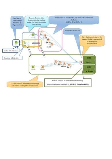
The groups of variables presented in Table 2, constituting conditional attributes, were used to build a model of prediction of final energy demand for building heating based on the Rough Set Theory. It was introduced in the 1980s by Professor Zdzisław Pawlak [45]. It is used as a tool to synthesize advanced and effective methods of analysis and to reduce datasets [48]. The rough sets serve as a methodology in the process of discovering knowledge in databases. It is a tool used to describe inaccurate, uncertain knowledge; to model decision-making systems; and for approximation reasoning [49]. The deduction methodology using the Approximate Collection Theory refers only to the qualitative nature of object characteristics. This causes limitations and difficulties when we deal with the occurrence of features in a quantitative form, not a qualitative one. The specificity of the attributes of the surveyed buildings shows a great variety of ways of encoding the given characteristics, which mostly occur in the quantitative form. In this case, the integration of the valued tolerance relation proves helpful [50]. It allows to implement more flexibility in data mining into the approximate set theory and to analyze observations expressed in quantitative form. The classic assumption of RSTs is based on the concept of the indistinguishability relationship as an exact relationship of equivalence, i.e., objects will only be indistinguishable if they have similar attributes (system 0–1). The introduction of a valued tolerance relation to RST allows to determine the upper and lower approximation of the crop with different degrees of indifference ratio [51]. This allows for the comparison of two sets of data and gives a result between 0 and 1, which is the level of indistinguishability. This range is a membership function derived from the assumptions of fuzzy harvest theory. The closer the result is to one, the more similar (indistinguishable) the objects are in terms of the analyzed attribute, and the closer to 0 the more distinguishable they are [50,51]. Detailed description of the prediction model based on quantitative variables has been presented in [51,52]. The general course of the construction of the model using the approximate sets theory is presented in Figure 1.
After selecting the possible list of independent variables (conditional attributes), the developed database was divided into a didactic set, to which 80% of the tested buildings were randomly selected, and a test set created from other objects. A schematic view of the work areas with individual blocks, illustrating the methodology for determining the energy demand indicator for heating after improvements based on the inference model built, is presented in Figure 2.
The evaluation of the quality of the developed model was assessed for individual groups of variables. For assessment of past due forecasts, the mean absolute error (MAE), mean absolute percentage error (MAPE)—also known as mean absolute percentage deviation (MAPD) [53,54]—as well as mean bias error (MBE), and coefficient of variance of the root mean square error (CV RMSE), was used; these are accepted as statistical calibration standards by ASHRAE Guideline 14-2002 [14,55,56]:
where: Or—real value of the index of final energy demand for heating after modernization (FE1); Opr—the forecast value of the index of final energy demand for heating after modernization; and ng—is the number of buildings covered by the study.
According to the ASHRAE Guideline, models are considered to be calibrated when MBE values are within ± 10% and CV RMSE values are within 30% [14,57].
The novelty of this research is an attempt to develop a universal model based on the rough set theory describing the final energy demand indicator for heating buildings and to use, for this purpose, groups of variables characterized by different degrees of difficulty in obtaining them. The algorithm of building a model for forecasting energy demand presented in the article allows decision-makers to assess the potential for real energy savings resulting from planned actions to improve thermal performance of existing buildings. It is important to underline the fact that, as the literature review shows, it has not yet been used in the energy assessment of buildings. The presented method based on Rough Set Theory (RST) should not be considered as competition for statistical analysis, but as an optional choice of method for data analysis. Bearing in mind that a common disadvantage of using classical statistical and data-based analyses is their time-consuming, costly nature (equipment and the collection of a sufficient, generally large number of representative observations), and the great complexity of the procedures used, which consists of so-called preliminary analyses (i.e., checking the assumptions of randomness of variables, examining the probability distribution and correct interpretation of statistical analysis results), as well as the ability to conduct and interpret statistical tests. In many cases, this results in the data being matched to the model, not the model to the data, as it should be in reality. When using rough set methods, the observations “speak for themselves” and are not corrected in any way, either before the application of the method or during the analysis. Moreover, the method based on RST is not limited, unlike regression models, by the number of sets of representative observations (both small and large sample of observations), nor is the construction of a statistical model required; decisions are made on the basis of dependencies: if certain conditions are met, a specific decision is taken (according to Boolean application). The presented method does not impose complicated rules of control of the features taken into account and the results of analyses. Only two main coefficients are used to control the significance of conditional attributes in relation to the decision attribute and the created decision rules: quality and approximation accuracy—easy to apply and interpret.
3. Results and Discussion
3.1. Analysis of Final Energy Consumption for Heating Buildings
The analyzed buildings are heated from the municipal heating network. Therefore, information on actual heat consumption for heating in the three heating seasons before and after the thermal modernization was obtained. On this basis, calculations of final energy demand for heating were made, and then the energy characteristics of objects in the state before and after thermal modernization were determined. To exclude seasonal fluctuations, the actual energy consumption values obtained were converted (corrected) to standard season conditions (multi-year average). The data concerning the heating season degree days (from the years 2010–2018 and the multiannual average) based on which the calculations were carried out were taken from the climate database Eurostat [58] for the Małopolska region.
The amount of final energy consumption was calculated using the formula:
where: QK,H —the final energy demand for the heating season, [kWh]; HDD(tb)0—the number of degree days in a standard heating season, [oCd]; HDD(tb)i—the number of degree days for the “i” of this year, [oCd]; QK,H i—final energy consumption for heating in a measurement period for the “i” of this year, [kWh].
The index of final energy demand for heating before and after the implementation of the improvement was calculated according to the formula:
where: FE—index of final energy demand for heating, [kWh·m−2·year−1]; QK,H—the final energy demand for the heating season, [kWh]; AH—calculated area of temperature-controlled rooms (heated surface), [m2].
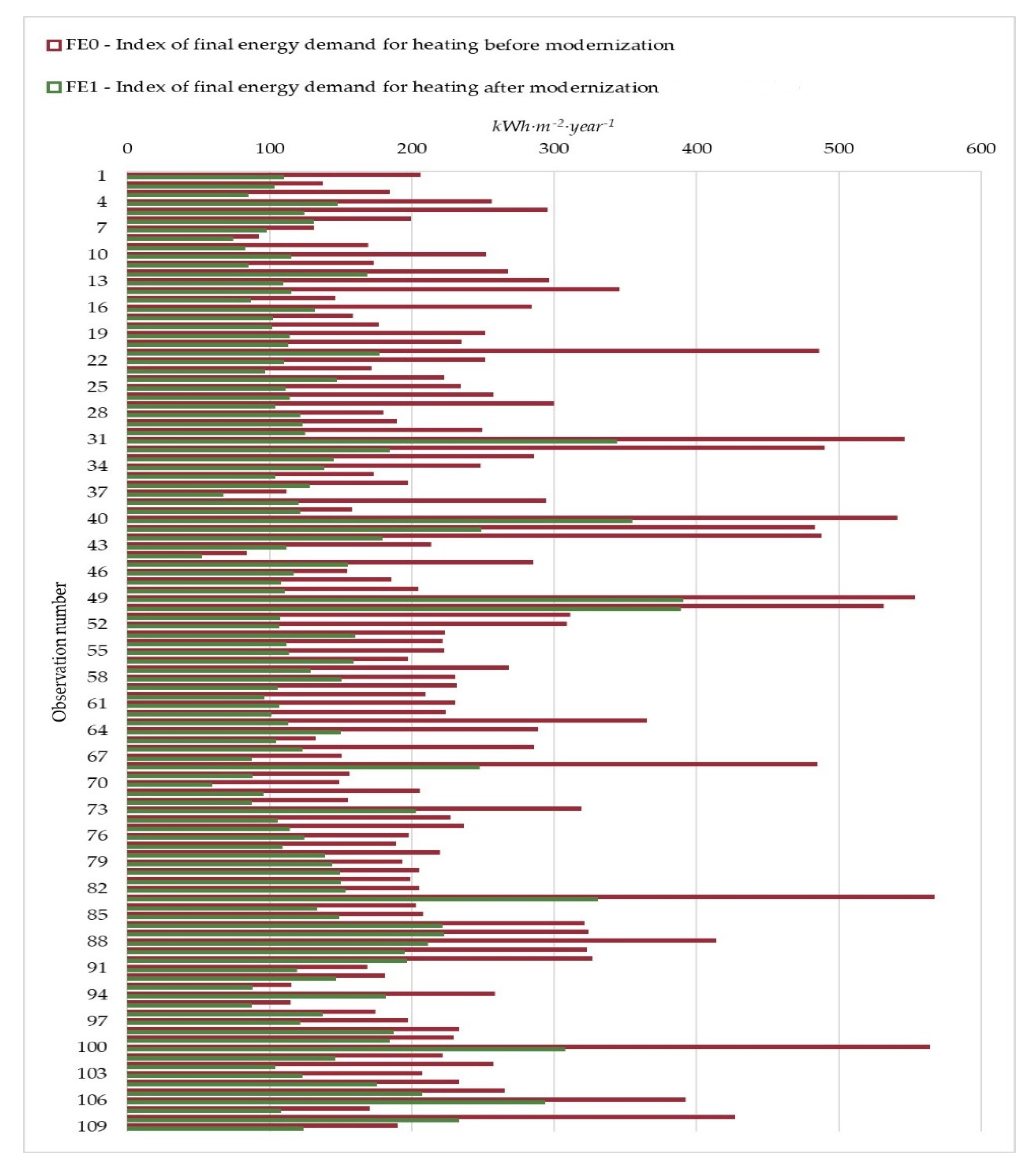
The energy characteristics of the analyzed group of buildings in the state before FE0 and after FE1 thermal modernization are shown in Figure 3. Figure 4 shows the structure of buildings in terms of energy consumption.
Index of final energy demand for heating of buildings is very varied. In buildings before modernization, it was between 83–569 [kWh·m−2·year−1], while after the improvement, it was 51–389 [kWh·m−2·year−1].
The average value of the index before modernization was 287 [kWh·m−2·year−1]; after the improvement, it decreased to 144 [kWh·m−2·year−1]. Average final energy consumption for heating an “average building” in Poland determined on the basis of a standard reference calculation based on EN ISO 13790/seasonal method [21] is: for buildings before thermal modernization 265.6 [kWh·m−2·year−1], while energy consumption after the improvement is 77.9 [kWh·m−2·year−1].
Nearly half of the buildings before the thermal modernization were characterized by energy consumption in the range 164–245 [kWh·m−2·year−1]. In the group of improved buildings, the largest group is made up of buildings where the energy demand for heating is between 99–147 [kWh·m−2·year−1].
Comparing the average values of the FE0 actual energy consumption index in the studied group of buildings with theoretical values, it can be seen that for existing buildings they are similar, whereas for improved buildings they differ. The projected energy consumption in a thermally improved “average building” based on standard reference calculations [46] is twice lower than the actual values.
3.2. Modeling the Consumption of Thermal Energy in Buildings Undergoing Energy Modernization
In the first part of the prediction model construction, the database was randomly divided into a teaching set and a test set. The input data characterizing the buildings were then divided into groups of variables Set I to Set IV. For individual groups from the learning set, the reducts and the core of the set of attributes were determined, which were used to create an inference model. The built model was subjected to a critical analysis (on the test set) in terms of accuracy and quality of the built forecast. The working space, on the basis of which the analyses were performed, is shown in Figure 2.
The results of quality and accuracy calculations of the constructed models depending on the selected set of input variables are shown in Table 3.
Analysis of the mean absolute values of the actual deviation of the final energy demand indicator for heating of residential buildings from the predicted value indicates that the model based on set IV has the lowest deviation value (18.1 kWh·m−2·year−1).
The highest error value (about 25.3 kWh·m−2·year−1) was shown by the model based on set III. The error value for the model based on the set I and II is similar and amounts to about 23 kWh·m−2·year−1.
The analysis of the MAPE error on the test set confirmed the usefulness of the model for determining the size of the energy demand indicator for heating for the building after thermal modernization. The obtained average error values for the selected Sets ranged from 14% to 17.8%.
The values of the two other meters used to assess the correctness of the models are as follows:
The MBE error values indicate that the energy consumption forecasts obtained from the model are overestimated for sets I, III and IV. The lowest value of the indicator (−0.73%) is obtained for set I, the highest (−16%) for set III. The model based on set II undervalued the actual values on average by 1.68%. The assessment of the energy demand indicator model expressed in the RSME CV ranges from 18.2% (Set II) to 32.2% (Set III).
Bearing in mind ASHARE’s recommendations for model calibration, it can be concluded that three models based on data sets meet the requirements. These are the models based on sets I, II and IV. The best values for the assessment indicators can be observed for the set II model and then for set I. An analysis of the assessment indicators (MBE and CV RSME, which are considered together) showed that the best value of the assessment indicators can be obtained for set II and then for set I. Set IV has a CV RMSE value close to set II, but the MBE value is clearly different from the others.
Taking all four assessment indicators into account, it can be seen that the best fit values are found for the model using the first set of variables.
4. Conclusions
The research was carried out on a group of 109 thermally improved residential buildings. The energy performance of these buildings was determined. The energy performance is based on the actual energy consumption for heating. The calculations were made for the state before and after thermal modernization. The specific sets of important variables characterizing the examined buildings have been identified. The variables were grouped into sets depending on the difficulty of obtaining them. They were used to build a prognostic model based on the rough set theory (RST). The use of this method made it possible to quickly determine the energy saving potential for heating after the completion of the thermal renovation.
The following conclusions can be drawn from the analysis of the indicators’ evaluation of the model for forecasting the final energy demand for heating after thermal improvement:
- The model developed based on the Rough Sets Theory (RST) is a universal solution that can be used for estimating thermal energy consumption in buildings undergoing thermal improvement. This is evidenced by the results of the assessment, where, according to the ASHRAE Guide, the calibration targets are set at ±10% (MBE) and less than 30% (CV RMSE). The achievement of these thresholds has been demonstrated for three models. These are models based on sets I, II and IV. The best results can be obtained for the model using sets II and I.
- Taking into account all four evaluation indicators, it was found that the best match between the predicted and real values can be obtained if a limited set of input variables (set I) is used in the model, the value of the deviation of the real value from the predicted value (MAE) is amounts to about 22.8 kWh·m−2·year−1, whereas the accuracy of estimation (MAPE) of the model built on the basis of these data is 15.4%. Similar forecasting results can be obtained by using the data set II, but in this case, a greater number of conditional attributes characterizing the building must be available.
- Analyzing the values of MAE and MAPE indicators, it was found that the best results for forecasting energy consumption after thermal improvement can be obtained using the IV set of input variables. The use of this set of variables to build the model allows obtaining the results with the error (MAE) 18.1 kWh·m−2·year−1. This gives an estimated accuracy (MAPE) of 14%. Despite this, this model is recommended as the third in order because of the high value of the MBE indicator, which clearly differs from the others.
- Forecasting the energy consumption of buildings using a model based on Rough Set Theory (RST) using variables that characterize buildings, allows for estimation accuracy of 14.4−15.9%. However, in further research, it is advisable to test this method on a larger, several hundred elementary set of objects (buildings) from different regions, characterized by different climatic conditions from those in which the research was performed, in order to verify the results obtained.
- The examined group of objects should be used to test other forecasting methods so that the results of the estimation can be compared with each other.
Author Contributions
Conceptualization, T.S.; software, T.S.; data curation, T.S.; investigation, T.S. and S.K.; methodology, T.S.; project administration, T.S. and S.K.; supervision, S.K.; writing—original draft, T.S. and S.K.; writing—reviewing and editing, S.K. and T.S. All authors have read and agreed to the published version of the manuscript.
Funding
This research was financed by the Ministry of Science and Higher Education of the Republic of Poland.
Acknowledgments
We are grateful to Sławomir Kurpaska from the University of Agriculture in Krakow, Poland, Faculty of Production and Power Engineering and Thomas G. Mathia from Laboratoire de Tribologie et Dynamique des Systèmes, École Centrale de Lyon, France for their valuable support during this research.
Conflicts of Interest
The authors declare no conflict of interest.
Nomenclature
| RST | Rough Set Theory |
| MAE | Mean Absolute Error |
| MAPE | Mean Absolute Percentage Error |
| MAPD | Mean Absolute Percentage Deviation |
| MBE | Mean Bias Error |
| CVRMSE | Coefficient of Variation of the Root Mean Square Error |
| Or | real value of the index of final energy demand for heating after modernization (FE1) |
| Opr | the forecast value of the index of final energy demand for heating after modernization |
| ng | number of buildings covered by the study |
| QK,H | final energy demand for the heating season |
| QK,H i | final energy consumption for heating in a measurement period for the “i” of this year |
| HDD(tb)0 | the number of degree days in a standard heating season |
| HDD(tb)i | the number of degree days for the “i” of this year |
| FE | index of final energy demand for heating |
| FE0 | index of final energy demand for heating before modernization |
| FE1 | index of final energy demand for heating after modernization |
| Af | calculated surface of heated floors from interior measurements |
| AH | calculated area of temperature-controlled rooms (heated surface) |
| Ar | calculated from exterior measurements surface of roof projection area (net) |
| Aw | calculated from exterior measurements total walls’ surface (net) area |
| Afl | calculated surface of floor from interior measurements (floor over basement or floor on the ground) |
| Atw | calculated from exterior measurements total windows area |
| Ve | calculated from exterior measurements the heated volume of building |
| S/Ve | shape coefficient of buildings (the ratio surface to volume) |
| NOs | number of stores |
| NOp | number of residential flats, premises |
| NOpb | number of living persons per building |
| Uw | calculated thermal transmittance of walls components |
| Upw | calculated thermal transmittance of peak walls components |
| Ur | calculated thermal transmittance of roof projections components |
| Ug | calculated thermal transmittance of floor components on the ground |
| Uf | calculated thermal transmittance of floors components (floor over basement) |
| Uwin | calculated thermal transmittance of windows (commercial data) |
| Φh | calculated heating consumed power |
References
- Act of 21 November 2008 on Support for Thermal Modernization and Renovation. Available online: http://prawo.sejm.gov.pl/isap.nsf/download.xsp/WDU20082231459/U/D20081459Lj.pdf (accessed on 3 November 2019).
- Directive 2010/31/EU of The European Parliament and of the Council of 19 May 2010 on the Energy Performance of Buildings. Available online: https://eur-lex.europa.eu/legal-content/PL/ALL/?uri=CELEX%3A32010L0031 (accessed on 3 November 2019).
- BGK. Figures of the Thermal Improvement and Repair Fund. 2018. Available online: https://www.bgk.pl/files/public/Pliki/Przedsiebiorstwa/fundusz_kredytu_technologicznego/Dane_liczbowe_FTiR.pdf (accessed on 29 November 2018).
- Bourdeau, M.; Zhai, X.-Q.; Nefzaoui, E.; Guo, X.; Chatellier, P. Modelling and forecasting building energy consumption: A review of data-driven techniques. Sustain. Sustain. Cities Soc. 2019, 48, 101533. [Google Scholar] [CrossRef]
- Fumo, N. A review on the basics of building energy estimation. Renew. Sustain. Energy Rev. 2014, 31, 53–60. [Google Scholar] [CrossRef]
- Foucquier, A.; Robert, S.; Suard, F.; Stéphan, L.; Jay, A. State of the art in building modelling and energy performances prediction: A review. Renew. Sustain. Energy Rev. 2013, 23, 272–288. [Google Scholar] [CrossRef] [Green Version]
- ASHRAE. ASHRAE Handbook–Fundamentals—Energy Estimation and Modeling Methods, SI ed.; American Society of Heating, Refrigerating and Air-Conditioning Engineers, Inc. (ASHRAE): Atlanta, GA, USA, 2009; ISBN 978-1-61583-170-8. Available online: https://app.knovel.com/web/toc.v/cid:kpASHRAE37/viewerType:toc/ (accessed on 5 November 2019).
- Ahmad, T.; Chen, H.; Guo, Y.; Wang, J. A comprehensive overview on the data driven and large scale based approaches for forecasting of building energy demand: A review. Energy Build. 2018, 165, 301–320. [Google Scholar] [CrossRef]
- Tardioli, G.; Kerrigan, R.; Oates, M.; O’Donnell, J.; Finn, D. Data Driven Approaches for Prediction of Building Energy Consumption at Urban Level. Energy Procedia 2015, 78, 3378–3383. [Google Scholar] [CrossRef] [Green Version]
- Yildiz, B.; Bilbao, J.I.; Sproul, A.B. A review and analysis of regression and machine learning models on commercial building electricity load forecasting. Renew. Sustain. Energy Rev. 2017, 73, 1104–1122. [Google Scholar] [CrossRef]
- Wang, J.; Srinivasan, R.S. A review of artificial intelligence based building energy use prediction: Contrasting the capabilities of single and ensemble prediction models. Renew. Sustain. Energy Rev. 2017, 75, 796–808. [Google Scholar] [CrossRef]
- Deb, C.; Lee, S.E. Determining key variables influencing energy consumption in office buildings through cluster analysis of pre-and post-retrofit building data. Energy Build. 2018, 159, 228–245. [Google Scholar] [CrossRef]
- Zhao, H.; Magoulès, F. A review on the prediction of building energy consumption. Renew. Sustain. Energy Rev. 2012, 16, 3586–3592. [Google Scholar] [CrossRef]
- Chang, C.; Zhu, N.; Yang, K.; Yang, F. Data and analytics for heating energy consumption of residential buildings: The case of a severe cold climate region of China. Energy Build. 2018, 172, 104–115. [Google Scholar] [CrossRef]
- Chalal, M.L.; Benachir, M.; White, M.; Shrahily, R. Energy planning and forecasting approaches for supporting physical improvement strategies in the building sector: A review. Renew. Sustain. Energy Rev. 2016, 64, 761–776. [Google Scholar] [CrossRef] [Green Version]
- Mat Daut, M.A.; Hassan, M.Y.; Hasimah, H.A.; Rahman, A.; Abdullah, M.P.; Hussin, F. Building electrical energy consumption forecasting analysis using conventional and artificial intelligence methods: A review. Renew. Sustain. Energy Rev. 2017, 70, 761–776. [Google Scholar] [CrossRef]
- CEN. Indoor Environmental Input Parameters for Design and Assessment of Energy Performance of Buildings Addressing Indoor Air Quality, Thermal Environment, Lighting and Acoustics; ISO 15251. 2008. Available online: https://standards.globalspec.com/std/1110417/EN%2015251 (accessed on 5 November 2019).
- Costanzoa, V.; Fabbrib, K.; Piraccini, S. Stressing the passive behavior of a Passivhaus: An evidence-based scenario analysis for a Mediterranean case study. Build. Environ. 2018, 142, 265–277. [Google Scholar] [CrossRef]
- Djamila, H. Indoor thermal comfort predictions: Selected issues and trends. Renew. Sustain. Energy Rev. 2017, 74, 569–580. [Google Scholar] [CrossRef]
- Wang, Y.; Kuckelkorn, J.; Zhao, F.-Y.; Spliethoff, H.; Lang, W. A state of art of review on interactions between energy performance and indoor environment quality in Passive House buildings. Renew. Sustain. Energy Rev. 2017, 72, 1303–1319. [Google Scholar] [CrossRef]
- CEN. European Standard: Energy Performance of Buildings-Calculation of Energy Use for Space Heating and Cooling. ISO 13790:2008. Available online: https://www.iso.org/standard/41974.html (accessed on 5 November 2019).
- CEN. European Standard: Heating Systems in Buildings; ISO 12831-1:2017-08; CEN: Brussels, Belgium, 2017. [Google Scholar]
- Ballarini, I.; Corrado, V. Application of energy rating methods to the existing building stock. Analysis of some residential buildings in Turin. Energy Build. 2009, 4, 790–800. [Google Scholar] [CrossRef]
- Crawley, D.B.; Lawrie, L.K.; Winkelmann, F.C.; Buhl, W.F.; Huang, Y.J.; Pedersen, C.O.; Strand, R.K.; Liesen, R.J.; Fisher, D.E.; Witte, M.J.; et al. Energyplus: Creating a new-generation building energy simulation program. Energy Build. 2001, 33, 319–331. [Google Scholar] [CrossRef]
- Rivers, N.; Jaccard, M. Combining top-down and bottom-up approaches to energy–economy modeling using discrete choice methods. Energy J. 2005, 26, 83–106. [Google Scholar] [CrossRef] [Green Version]
- Geysena, D.; De Somera, O.; Johanssonc, C.; Bragec, J.; Vanhoudta, D. Operational thermal load forecasting in district heating networks using machine learning and expert advice. Energy Build. 2017, 162, 144–153. [Google Scholar] [CrossRef]
- Allard, I.; Olofsson, T.; Hassan, O.A.B. Methods for energy analysis of residential buildings in Nordic countries. Renew. Sustain. Energy Rev. 2013, 22, 306–318. [Google Scholar] [CrossRef]
- Asadi, S.; Amiri, S.S.; Mottahedi, M. On the development of multi-linear regression analysis to assess energy consumption in the early stages of building design. Energy Build. 2014, 85, 246–255. [Google Scholar] [CrossRef]
- Asadi, S.; Marwa, H.; Beheshti, A. Development and validation of a simple estimating tool to predict heating and cooling energy demand for attics of residential buildings. Energy Build. 2012, 54, 12–21. [Google Scholar] [CrossRef]
- Caldera, M.; Corgnati, S.P.; Filippi, M. Energy demand for space heating through a statistical approach: Application to residential buildings. Energy Build. 2008, 40, 1972–1983. [Google Scholar] [CrossRef]
- Chou, J.S.; Bui, D.K. Modeling heating and cooling loads by artificial intelligence for energy-efficient building design. Energy Build. 2014, 82, 437–446. [Google Scholar] [CrossRef]
- Fumo, N.; Biswas, R. Regression analysis for prediction of residential energy consumption. Renew. Sustain. Energy Rev. 2015, 47, 332–343. [Google Scholar] [CrossRef]
- Lü, X.; Lu, T.; Kibert, C.J.; Viljanen, M. Modeling and forecasting energy consumption for heterogeneous buildings using a physical–statistical approach. Appl. Energy 2015, 144, 261–275. [Google Scholar] [CrossRef]
- Ma, Z.; Li, H.; Sun, Q.; Wang, C.; Yan, A.; Starfelt, F. Statistical analysis of energy consumption patterns on the heat demand of buildings in district heating systems. Energy Build. 2014, 85, 464–472. [Google Scholar] [CrossRef]
- Praznik, M.; Butala, V.; Zbašnik-Senegačnik, M. Simplified evaluation method for energy efficiency in single-family houses using key quality parameters. Energy Build. 2013, 67, 489–499. [Google Scholar] [CrossRef]
- Sekhar-Roy, S.; Roy, R.; Balas, V.E. Estimating heating load in buildings using multivariate adaptive regression splines, extreme learning machine, a hybrid model of mars and elm. Renew. Sustain. Energy Rev. 2018, 82, 4256–4268. [Google Scholar] [CrossRef]
- Tiberiu, C.; Virgone, J.; Blanco, E. Development and validation of regression models to predict monthly heating demand for residential buildings. Energy Build. 2008, 40, 1825–1832. [Google Scholar] [CrossRef]
- Tsanas, A.; Xifara, A. Accurate quantitative estimation of energy performance of residential buildings using statistical machine learning to OLS. Energy Build. 2012, 49, 560–567. [Google Scholar] [CrossRef]
- Biswas, M.; Robinson, M.D.; Fumo, N. Prediction of residential building energy consumption: A neural network approach. Energy 2016, 117, 84–92. [Google Scholar] [CrossRef]
- Ekici, B.B.; Aksoy, U.T. Prediction of building energy consumption by using artificial neural networks. Adv. Eng. Softw. 2009, 40, 356–362. [Google Scholar] [CrossRef]
- Li, K.; Sua, H.; Chua, J. Forecasting building energy consumption using neural networks and hybrid neuro-fuzzy system: A comparative study. Energy Build. 2011, 43, 2893–2899. [Google Scholar] [CrossRef]
- Kumar, R.; Aggarwal, R.K.; Sharma, J.D. Energy analysis of a building using artificial neural network: A review. Energy Build. 2013, 65, 352–358. [Google Scholar] [CrossRef]
- Seyedzadeh, S.; Rahimian, F.; Glesk, I.; Roper, M. Machine learning for estimation of building energy consumption and performance: A review. Vis. Eng. 2018, 6, 5. [Google Scholar] [CrossRef]
- Mihai, M.; Tanasiev, V.; Dinca, C.; Badea, A.; Vidu, R. Passive house analysis in terms of energy performance. Energy Build. 2017, 144, 74–86. [Google Scholar] [CrossRef]
- Pawlak, Z. Rough Sets. Theoretical Aspects of Reasoning about Data; Kluwer Academic Press: Dordrecht, The Netherlands, 2012; Available online: http://bcpw.bg.pw.edu.pl/Content/2026/RoughSetsRep29.pdf (accessed on 5 November 2019).
- TABULA. Polish building typology. In Scientific Report; Narodowa Agencja Poszanowania Energii: Warszawa, Poland, 2012. Available online: https://episcope.eu/fileadmin/tabula/public/docs/scientific/PL_TABULA_ScientificReport_NAPE.pdf (accessed on 15 January 2020).
- Comparison of Typical Buildings from Evaluation of the TABULA Database and Heat Supply Systems 20 European Countries TABULA Evaluation of the Database. Available online: https://episcope.eu/fileadmin/tabula/public/docs/report/TABULA_WorkReport_EvaluationDatabase.pdf (accessed on 15 January 2020).
- Nutech Solution-Science for Business. 2005. Available online: http://www.nutechsolutions.com.pl/ (accessed on 10 October 2019).
- Nguyen, H.S. Tolerance Rough Set Model and Its Applications in Web Intelligence. In Proceedings of the IEEE/WIC/ACM International Joint Conferences on Web Intelligence (WI) and Intelligent Agent Technologies (IAT), Atlanta, GA, USA, 17–20 November 2013; IEEE CS: Washington, DC, USA, 2013; pp. 237–244. [Google Scholar] [CrossRef]
- Nguyen, D.V.; Yamada, K.; Unehara, M. Extended Tolerance Relation to Define a New Rough Set Model in Incomplete Information Systems. AFS 2013, 2013, 372091. [Google Scholar] [CrossRef] [Green Version]
- Renigier-Biłozor, M. Zastosowanie teorii zbiorów przybliżonych do masowej wyceny nieruchomości na małych rynkach (Application of rough set theory for mass valuation of real estate in small markets). Acta Sci. Pol. Adm. Locorum 2008, 7, 35–51. [Google Scholar]
- Szul, T.; Nęcka, K.; Knaga, J. Application of Rough Set Theory to Establish the Amount of Waste in Households in Rural Areas. Ecol. Chem. Eng. S 2017, 24, 311–325. [Google Scholar] [CrossRef] [Green Version]
- Dittmann, P. Prognozowanie w Przedsiębiorstwie; Wolters Kluwer Polska Sp. z o.o.: Kraków, Poland, 2008. [Google Scholar]
- Cieślak, M. Prognozowanie Gospodarcze; Wydawnictwo Naukowe PWN: Warszawa, Poland, 1999. [Google Scholar]
- Ruiz, G.R.; Bandera, C.R. Validation of Calibrated Energy Models: Common Errors. Energies 2017, 10, 1587. [Google Scholar] [CrossRef] [Green Version]
- ASHRAE. ASHRAE Guideline 14-2002 for Measurement of Energy and Demand Savings; American Society of Heating, Refrigeration and Air Conditioning Engineers: Atlanta, GA, USA, 2002. [Google Scholar]
- ASHRAE. American Society of Heating, Ventilating, and Air Conditioning Engineers (ASHRAE). Guideline 14-2014, Measurement of Energy and Demand Savings; Technical Report; American Society of Heating, Ventilating, and Air Conditioning Engineers: Atlanta, GA, USA, 2014. [Google Scholar]
- European Union Statistics, Eurostat. Cooling and Heating Degree Days by NUTS 2 Regions—Annual Data. Available online: http://data.europa.eu/88u/dataset/7kv8vguICyNRJYqLRzzFw (accessed on 30 November 2019).
Figure 1.
Diagram for building of a model of inference based on the core of a set of conditional attributes using the theory of rough sets.
Figure 1.
Diagram for building of a model of inference based on the core of a set of conditional attributes using the theory of rough sets.

Figure 2.
View of the working space.

Figure 3.
Index of final energy demand for heating of buildings before and after implementing improvements.
Figure 3.
Index of final energy demand for heating of buildings before and after implementing improvements.

Figure 4.
Structure of buildings due to the size of the energy demand indicator for heating (a) before (b) after the improvement.
Figure 4.
Structure of buildings due to the size of the energy demand indicator for heating (a) before (b) after the improvement.


Table 1.
Characteristics of the selected values that influence the reduction of annual energy demand for buildings subjected to thermal efficiency improvement.
Table 1.
Characteristics of the selected values that influence the reduction of annual energy demand for buildings subjected to thermal efficiency improvement.
| No. | Parameter | Abbreviation | Average | Median |
|---|---|---|---|---|
| 1 | calculated surface of heated floors from interior measurements, [m2] | Af | 1567.4 | 1524.2 |
| 2 | calculated area of temperature-controlled rooms (heated surface), [m2] | AH | 1764.0 | 1565.4 |
| 3 | calculated from exterior measurements surface of roof projection area (net), [m2] | Ar | 467.0 | 383.1 |
| 4 | calculated from exterior measurements total walls’ surface (net) area, [m2] | Aw | 1096.6 | 979.8 |
| 5 | calculated surface of floor from interior measurements (floor over basement or floor on the ground), [m2] | Afl | 395.4 | 360 |
| 6 | calculated from exterior measurements total windows area, [m2] | Atw | 290.5 | 251.1 |
| 7 | calculated from exterior measurements the heated volume of building, [m3] | Ve | 6391.6 | 5408.8 |
| 8 | shape coefficient of buildings (the ratio surface to volume), [m2·m−3], [m−1] | S/Ve | 0.46 | 0.42 |
| 9 | number of stores, [pc.] | NOs | 4.3 | 4 |
| 10 | number of residential flats, premises [pc.] | NOp | 32.4 | 29 |
| 11 | number of living persons per building [Nb] | NOpb | 73.9 | 64 |
| 12 | calculated thermal transmittance of walls components, [W·m−2·K−1] | Uw | 1.12 | 1.16 |
| 13 | calculated thermal transmittance of peak walls components, [W·m−2·K−1] | Upw | 1.0 | 0.94 |
| 14 | calculated thermal transmittance of roof projections components, [W·m−2·K−1] | Ur | 1.24 | 0.72 |
| 15 | calculated thermal transmittance of floor components on the ground, [W·m−2·K−1] | Ug | 1.62 | 1.41 |
| 16 | calculated thermal transmittance of floors components (floor over basement), [W·m−2·K−1] | Uf | 1.13 | 1.1 |
| 17 | calculated thermal transmittance of windows (commercial data), [W·m−2·K−1] | Uwin | 1.82 | 1.6 |
| 18 | calculated heating consumed power, [kW] | Φh | 189.2 | 161.2 |
| 19 | measured, the annual heat consumption for building heating converted (according to formula 3) to the conditions of the standard heating season, [MWh·year−1] | QK,H0 | 506.6 | 475.3 |
Table 2.
Sets of input variables for analyzed predictive models. Sets of variables (before thermal modernization) (Recorded in the form of 0–1 information—whether the peak wall, external wall, floors, ground floors, windows, and flat roof are to be thermal modernized).
Table 2.
Sets of input variables for analyzed predictive models. Sets of variables (before thermal modernization) (Recorded in the form of 0–1 information—whether the peak wall, external wall, floors, ground floors, windows, and flat roof are to be thermal modernized).
| Parameter-Condition Attributes | |
|---|---|
| Set I | Φh – calculated heating consumed power, [kW] FE0 – index of final energy demand for heating before modernization, [kWh·m−2·year−1] |
| Set II | Ve – calculated from exterior measurements the heated volume of building, [m3] S/Ve – shape coefficient of buildings (the ratio surface to volume), [m2·m−3], [m−1] Af – calculated surface of heated floors from interior measurements, [m2] Aw – calculated from exterior measurements total walls’ surface (net) area, [m2] Ar – calculated from exterior measurements surface of roof projection area (net), [m2] Atw – calculated from exterior measurements total windows area, [m2] Ain – calculated from interior measurements total (net internal area), [m2] Nopb – number of living persons per building, [Nb] Nop – number of residential flats, premises, [pcs.] FE0 – index of final energy demand for heating before modernization, [kWh·m−2·year−1] |
| Set III | Uw – calculated thermal transmittance of walls components, [W·m−2·K−1] Upw – calculated thermal transmittance of peak walls components, [W·m−2·K−1] Ur – calculated thermal transmittance of roof projections components, [W·m−2·K−1] Uf – calculated thermal transmittance of floors components (floor over basement), [W·m−2·K−1] Uwin – thermal transmittance of windows (commercial data), [W·m−2·K−1] Ug – calculated thermal transmittance of floor components on the ground, [W·m−2·K−1] Ve – calculated from exterior measurements the heated volume of building, [m3] S/Ve – shape coefficient of buildings (the ratio surface to volume), [m2·m−3], [m−1] Af – calculated surface of heated floors from interior measurements, [m2] Aw – calculated from exterior measurements total walls’ surface (net) area, [m2] Ar – calculated from exterior measurements surface of roof projection area (net), [m2] Atw – calculated from exterior measurements total windows area, [m2] Ain – calculated from interior measurements total (net internal area), [m2] Nopb – number of living persons per building, [Nb] Nop – number of residential flats, premises, [pc.] FE0 – index of final energy demand for heating before modernization, [kWh·m−2·year−1] |
| Set IV | Uw – calculated thermal transmittance of walls components, [W·m−2·K−1] Upw – calculated thermal transmittance of peak walls components, [W·m−2·K−1] Ur – calculated thermal transmittance of roof projections components, [W·m−2·K−1] Uf – calculated thermal transmittance of floors components (floor over basement), [W·m−2·K−1] Uwin – thermal transmittance of windows (commercial data), [W·m−2·K−1] Ug – calculated thermal transmittance of floor components on the ground, [W·m−2·K−1] Af – calculated surface of heated floors from interior measurements, [m2] Aw – calculated from exterior measurements total walls’ surface (net) area, [m2] Ar – calculated from exterior measurements surface of roof projection area (net), [m2] Atw – calculated from exterior measurements total windows area, [m2] FE0 – index of final energy demand for heating before modernization, [kWh·m−2·year−1] |
Table 3.
Assessment of model of energy demand indicator for heating based on studied set of input variables (Set I to Set IV).
Table 3.
Assessment of model of energy demand indicator for heating based on studied set of input variables (Set I to Set IV).
| Assessment Parameters | Sets of variables | |||
|---|---|---|---|---|
| Set I | Set II | Set III | Set IV | |
| MAE [kWh·m−2·year−1] | 22.8 | 23.1 | 25.3 | 18.1 |
| MAPE [%] | 15.4 | 16.4 | 17.8 | 14 |
| MBE [%] | −0.73 | 1.68 | −16 | −9.6 |
| CV RMSE [%] | 21.7 | 18.2 | 32.2 | 18.8 |
© 2020 by the authors. Licensee MDPI, Basel, Switzerland. This article is an open access article distributed under the terms and conditions of the Creative Commons Attribution (CC BY) license (http://creativecommons.org/licenses/by/4.0/).
Share and Cite
MDPI and ACS Style
Szul, T.; Kokoszka, S. Application of Rough Set Theory (RST) to Forecast Energy Consumption in Buildings Undergoing Thermal Modernization. Energies 2020, 13, 1309. https://0-doi-org.brum.beds.ac.uk/10.3390/en13061309
AMA Style
Szul T, Kokoszka S. Application of Rough Set Theory (RST) to Forecast Energy Consumption in Buildings Undergoing Thermal Modernization. Energies. 2020; 13(6):1309. https://0-doi-org.brum.beds.ac.uk/10.3390/en13061309
Chicago/Turabian StyleSzul, Tomasz, and Stanisław Kokoszka. 2020. "Application of Rough Set Theory (RST) to Forecast Energy Consumption in Buildings Undergoing Thermal Modernization" Energies 13, no. 6: 1309. https://0-doi-org.brum.beds.ac.uk/10.3390/en13061309
Note that from the first issue of 2016, this journal uses article numbers instead of page numbers. See further details here.