Discrete Element Method Investigation of Binary Granular Flows with Different Particle Shapes
by

Yi Liu
1, 
Zhaosheng Yu
1,
Jiecheng Yang
2,
Carl Wassgren
3,
Jennifer Sinclair Curtis
2 and
Yu Guo
1,* 1
Department of Engineering Mechanics, Zhejiang University, Hangzhou 310027, China
2
Department of Chemical Engineering, University of California Davis, Davis, CA 95616, USA
3
School of Mechanical Engineering, Purdue University, West Lafayette, IN 47907, USA
*
Author to whom correspondence should be addressed.
Energies 2020, 13(7), 1841; https://0-doi-org.brum.beds.ac.uk/10.3390/en13071841
Submission received: 10 March 2020
/
Revised: 2 April 2020
/
Accepted: 7 April 2020
/
Published: 10 April 2020
(This article belongs to the Special Issue DEM of Multiphase Flows and Powder Processing)
Abstract
:The effects of particle shape differences on binary mixture shear flows are investigated using the Discrete Element Method (DEM). The binary mixtures consist of frictionless rods and disks, which have the same volume but significantly different shapes. In the shear flows, stacking structures of rods and disks are formed. The effects of the composition of the mixture on the stacking are examined. It is found that the number fraction of stacking particles is smaller for the mixtures than for the monodisperse rods and disks. For binary mixtures with small particle shape differences, the mixture stresses are bounded by the stresses of the two corresponding monodisperse systems. However, for binary mixtures with large particle shape differences, the stresses of the mixtures can be larger than the stresses of the monodisperse systems at large solid volume fractions because larger differences in particle shape cause geometrical interference in packing, leading to stronger particle–particle interactions in the flow. The stresses in dense binary mixtures are found to be exponential functions of the order parameter, which is a measure of particle alignment. Based on the simulation results, an empirical expression for the bulk friction coefficient (ratio of the shear stress to normal stress) for dense binary flows is proposed by accounting for the effects of particle alignment and solid volume fraction.

1. Introduction
Granular shear flows are prevalent in natural and industrial processes, such as snow avalanches, landslides, sand storms, mineral transport, chemical and pharmaceutical processing, coal combustion, and food production. Studies on the mechanics and physics of granular flows have been carried out because a good understanding of the granular flow properties is useful to control damage caused by natural disasters and to optimize industrial processes. Theories of granular flow rheology have been developed. By treating particles as gas molecules, the kinetic theory of gases was introduced to statistically describe mechanical and thermal properties of dilute, dry granular flows [1], and the theory was thereafter extended to the dense flow regime [2,3]. Jop et al. [4] found that the ratio of shear to normal stress, , was a function of the inertial number, , in which is local shear rate, is local pressure, and and are particle diameter and density, respectively. Thus, the constitutive relation for dense flows is described by the correlation , which is well known as the -theory. Non-local effects have been considered in subsequent work [5,6]. Recently, Pähtz et al. [7] observed that the ratio of shear to normal stress, , scaled with the square root of the local Péclet number, , for dry, wet, dilute, and dense granular flows, provided that the particle diameter exceeds the particle mean free path.
Most granular materials are mixtures containing particles of different sizes, densities, shapes, and elastic moduli. The flow behavior of mixtures can be distinct from that of monodisperse systems. Shen [8] derived a set of constitutive equations for the stresses in a rapid flow of spherical particles with two sizes based on the assumptions: (i) binary collisions are the major stress-generating mechanism; (ii) stresses are caused by momentum exchange between surface particles and exterior particles; (iii) the work done by shear stresses on the boundaries is balanced by the energy dissipation through particle–particle collisions; and (iv) a larger particle and a smaller particle have the same random fluctuation energy, i.e., equipartition of energy. The predictions by Shen’s theory was good for a diameter ratio close to unity and deteriorated for large particle size differences, as pointed out in [9]. Jenkins and Mancini [9] and Farrell et al. [10] extended the kinetic theory, which was developed for monodisperse systems [1], to describe granular flows of binary mixtures. In the work of Farrell et al. [10], equipartition of energy between different particle species was also assumed and a radial distribution function at contact was defined as a function of the sizes and solid concentrations of the two particle species. Compared with experimental results, the prediction of Farrell et al. [10] was in good agreement at small solid volume fractions, but significant discrepancies at large solid volume fractions were observed due to the dominance of enduring contacts, which violated the binary collision assumption. In the kinetic theory of Jenkins and Mancini [9], it was assumed that the pair distribution function for two 2D disks is the product of Maxwellian velocity distributions and a factor that accounts for the effects of excluded area and collisional shielding, and non-equipartition of energy is considered. Compared to Shen’s work [8], the theory of Jenkins and Mancini can correctly predict that the stresses decrease with an increase in small particle concentration over a much wider range of particle diameter ratios. By incorporating the Revised Enskog Theory [11] and using non-Maxwellian velocity distributions, Willits and Arnarson [12] developed another version of kinetic theory, which showed better agreement with the discrete particle simulation results than the Jenkins-Mancini theory [9]. Shear flow simulations of binary mixtures [13] showed that equipartition of energy between large and small particles rapidly deteriorated as the coefficient of restitution decreased and the particle size difference increased. Galvin et al. [14] evaluated the effect of non-equipartition of energy on rapid flows of granular mixtures. It was found that for simple shear flows without segregation, the prediction from kinetic theory was insensitive to the equipartition versus non-equipartition treatment, while for segregating flows the presence of non-equipartition gave rise to additional components of the driving forces for the size segregation, resulting in better predictions. Thus, non-equipartition of energy should be considered in kinetic theory for describing a wide range of polydisperse granular flows. Iddir and Arastoopour [15] considered non-Maxwellian velocity distributions and non-equipartition in their kinetic theory. By comparing four different kinetic theories of granular mixtures, Benyahia [16] demonstrated that the Iddir–Arastoopour theory gave the best prediction of the discrete particle simulations.
Dense flows of granular mixtures were computationally investigated using the Discrete Element Method (DEM) by Tripathi and Khakhar [17] and Gu et al. [18]. It was found that like monodisperse dense flows, polydisperse dense flows also followed a -like rheological correlation, in which the shear to normal stress ratio is a function of the inertial number . However, the yielding stress ratio in the model depended on the polydispersity and skewness of the particle size distribution [18]. Dahl et al. [19,20] explored the effects of continuous size distributions on rapid granular flows using numerical simulations of simple shear flows. It was observed that the stresses with Gaussian and lognormal size distributions were consistent with the stresses of monodisperse systems when the root-mean-square (2D) or root-mean-cubed (3D) particle diameter of the mixture was equal to the diameter of the monodisperse system. A similar conclusion was also obtained from the kinetic theory of Farrell et al. [10].
Previous work of granular mixtures mainly focused on differences in particle size and density, and the effects of particle shape differences in a mixture were much less studied. Yang et al. [21] performed DEM simulations of shear flows of binary mixtures with large oval and rod-like particles and small spheres. They found that the particle projected area in the plane perpendicular to the flow direction played an important role. The stress–solid volume fraction curves of binary mixtures with different volume ratios of small-to-large particle species collapsed on a single master curve by normalizing the stresses using the effective particle projected area and root-mean-cubed diameter. Shear flows of mixtures of cylindrical particles were studied using DEM by Hao et al. [22]. In these mixtures, the cylindrical particles had the same diameter but different lengths. It was observed that the interaction between different particle species increased the alignment of shorter particles and reduced the alignment of longer particles. The total stress tensor of a mixture could be expressed as a sum of the stress tensors of the monodispersed particle species, which were linearly scaled by the concentrations of the corresponding species.
For an improved understanding of the effects of particle shape differences, shear flows of binary mixtures of elongated rods and flat disks are simulated using DEM in the present work. In these binary mixtures, a rod has the same volume as a disk, and thus all the particles have the same equivalent volume diameter . Therefore, the effects of particle size differences are eliminated and only particle shape differences exist in the mixtures. In the shear flows, the rods and disks exhibit significant stacking and alignment. The effects of the composition in a mixture on the stacking and alignment behaviors and the particle-phase stresses are then explored. Lastly, a correlation between the microstructure and the stresses is investigated.
2. Methodology
2.1. Cylindrical Particle Discrete Element Method
The Discrete Element Method (DEM), which was first proposed by Cundall and Strack [23], is a popular numerical tool for studying particulate systems. In DEM, the motion of each particle is incrementally solved by time integration, and the contact forces between the particles need to be determined in each time step. Based on the algorithms of contact detection for cylindrical objects presented by Kodam et al. [24] and Guo et al. [25], an in-house DEM code is developed and utilized in this work for the modeling of cylindrical particles. In this method, the translational and rotational motion of an individual particle i is described based on Newton’s law of motion,
where vi and ωi are the translational and angular velocities of the particle i, respectively. The translational movement of the particle of the mass mi is driven by the contact force , and the rotation is induced by the torque Ti generated from the contact forces (including both normal and tangential forces for a cylindrical particle). For 3D non-spherical particles, the parameter Ii is the moment of inertia tensor. The velocities and positions of the particles can be updated by the time integration of Equations (1) and (2) with a fixed time step. The orientation of a cylindrical particle is described by a rotation matrix and updated by the current angular velocity at each time step [26].
The geometries of cylindrical particles in the DEM simulations are illustrated in Figure 1. The aspect ratio (AR) of a cylinder is defined as the ratio of particle length to diameter, i.e., . Thus, a rod and a disk correspond to AR > 1 and AR < 1, respectively. Six typical contact types exist for the contact between two cylindrical particles [24]: face–face, face–band, face–edge, band–band (parallel and skewed), band–edge, and edge–edge. In addition, several special contact types were recognized [25]. The algorithms to determine overlap size, contact normal direction, and contact point position for each contact type, which are provided in [24,25], are summarized for convenience in Appendix A. The overlap size is used to calculate the normal contact force based on the Hertz model [27],
where
In Equation (4), E1, E2 and ζ1, ζ2 are the Young’s moduli and Poisson’s ratios of the two particles in contact, respectively. In Equation (5), and represent the radii of the two cylindrical particles in contact. To consider the dissipation of kinetic energy in the particle–particle contact process, a damping force is added to the normal contact force, which has the expression,
where
and is the normal component of the relative velocity at the contact point between two particles. In Equation (8), and are the masses of two contacting particles. The damping coefficient β in Equation (6) is a function of coefficient of normal restitution (i.e., the ratio of post-collisional to pre-collisional the relative normal velocity at the contact point).
In this study, the cylindrical particles are frictionless without tangential contact forces. It should be noted that the same contact force models of Equations (3) and (6) are used for each contact type without considering the difference in contact geometry. This simplification works well for a number of packing and flow processes as discussed in the following section.
2.2. DEM Code Validation
To validate the present DEM code, particle packing, hopper discharge, and granular shear flow with the cylindrical particles were simulated in our previous studies. In the particle packing [28], cylindrical particles were dropped into a cylindrical container one-by-one, and the packing density was evaluated after all the particles settled with nearly zero velocities. The packing densities of AR = 6 cylinders obtained from the DEM simulations were consistent with experimental results for two different dropping heights. In the hopper discharge of cylindrical particles with different particle aspect ratios [29], similar particle discharge rates were obtained for the DEM simulations and experiments. Simple shear flows of monodispersed cylinders were also simulated using the present code [30]. It was observed that the stresses of the cylindrical particles with AR = 1 were close to the prediction of kinetic theory [1], which usually predicts the stresses of spheres. This consistency is reasonable as the difference in sphericity is small between the spheres and the cylinders with AR = 1. It was also observed that the stress discrepancy between the spheres and the cylinders increased as the sphericity of the cylinders decreased (i.e., as AR increased). This dependence of stresses on particle sphericity was qualitatively consistent with previous findings [31]. As a result, the algorithms used in the present cylindrical particle DEM code are verified as the agreement is achieved between the simulation and experimental results.
2.3. Computational Set-up of Shear Flow
Shear flows of binary mixtures of rods and disks in the absence of an interstitial fluid are simulated using the DEM code. The gravitational force is switched off in order to achieve a uniform field of stress and particle distribution in the shear domain. As shown in Figure 2, a well-mixed binary mixture of rods and disks is uniformly generated in a rectangular domain of dimensions Lx = 0.0072 m, Ly = 0.0072 m, and Lz = 0.0036 m (i.e., Lx/dv = 30.25, Ly/dv = 30.25, and Lz/dv = 15.13). The properties of the rods (AR = 6) and disks (AR = 0.1, 0.15, 0.2, and 0.3) are presented in Table 1. All of the particles have the same volume and thus the same equivalent volume diameter dv. An approach to generate a uniform, densely packed bed of cylindrical particles in a specified domain was proposed in [25].
In the simulations, shear flow is initiated by applying a linear x-velocity profile of particles in the y-direction,
where is the x-component of the velocity of particle i, is the assigned shear rate, and are the y-coordinate of the mass center of particle i and the y-coordinate of the center of the shear domain, respectively. Periodic boundary conditions are used in the x and z directions, and a Lees–Edwards boundary condition [32] is specified in the y-direction. According to the Lees–Edwards boundary condition, when the mass center of a particle moves out of the upper (or lower) boundary, it is reintroduced into the shear domain from the lower (or upper) boundary with the particle x-velocity minus (or plus) , by which a constant average shear rate is maintained in the domain. Meanwhile, the x-coordinate of the reintroduced particle is modified to account for the cumulative shear deformation [32], the y-coordinate is minus (or plus) , and the z-coordinate remains unchanged. Thus, a granular shear flow occurs in the x-y plane. It is noted that during the shear flow process, the particle x-velocity profile always maintains approximately linear as described by Equation (10).
In the shear flow simulations, the average stress tensor of the particle phase within the shear domain can be measured. The total stress tensor consists of a kinetic component and a collisional component , i.e., . The kinetic component arises from the particle velocity fluctuation and is written as,
in which is the fluctuating velocity of particle i, and represents average particle velocity in a local steady state, which can be determined using Equation (10) because the average velocity profile follows such a profile at the steady state. The parameter N is the total number of particles in the domain of total volume and ⊗ represents the dyadic product operator.
The collisional stress tensor, which arises from the particle–particle contact forces, is given by
in which is the contact force, is a vector connecting the centers of mass of two contacting particles, and is the number of contacts. A steady state of shear flow occurs when a balance is reached between shear production (from the upper and lower boundaries) and energy dissipation (via particle–particle collisions). At the steady state, the physical quantities, such as stresses and number of contacts, fluctuate slightly around constant values.
2.4. Sensitivity to Time Step and Domain Size
In previous DEM simulations with spherical particles, a critical time step was determined based on the Rayleigh wave propagation on a particle [33]. In this work, a critical time step for DEM modeling of cylindrical particles is proposed by a simple modification to the expression of critical time step for spherical particles,
where the characteristic particle size is the minimum value between the cylindrical particle diameter and length , and is the shear modulus (). The real time step used in the simulations is usually a small fraction of the critical time step, i.e., , in which is between 0 and 1. Different time steps of = 0.025, 0.05, 0.075, 0.1, 0.3, and 0.6 are used to check the sensitivity in the shear flow simulations of the binary mixture of AR = 0.3, AR = 6 and C = 0.5 at the solid volume fraction = 0.4. The rods fraction C is defined as the number fraction of rods, i.e., , in which and are the numbers of rods and disks, respectively, in a binary mixture. As shown in Figure 3a, the total shear stresses , normalized by , are nearly unaffected by the four different time steps, indicating that numerical convergence has been achieved. Thus, a relatively larger time step with = 0.1 is chosen for the rest of simulations in order to reduce the computational cost.
The base shear flow domain has the dimensions [Lx = 30.25 dv, Ly = 30.25 dv, Lz = 15.13 dv]. To examine the effect of domain size, two larger domains are considered: [1.5Lx, 1.5Ly, 1.5Lz] and [2Lx, 2Ly, 2Lz]. A comparison of simulation results with the three different domains is made in Figure 3b. It can be seen that a similar evolution of normalized shear stress is obtained and the average stresses at steady state are nearly the same with the three different domains. Therefore, the base flow domain is sufficiently large to produce domain size-independent results. The stress results of a dilute flow at = 0.05 are shown in Figure 3b. Nevertheless, the domain of [Lx = 30.25 dv, Ly = 30.25 dv, Lz = 15.13 dv] can also produce the domain size-independent results for the dense flows, due to the fact that a larger number of particles (in a dense flow than in a dilute flow) leads to a better statistical evaluation. As a result, the base domain of dimensions [Lx = 30.25 dv, Ly = 30.25 dv, Lz = 15.13 dv] has been used for all the shear flow simulations reported in the following sections. In the shear flow process, the volume of the shear domain is kept constant.
3. Particle Stacking and Alignment
In dense shear flows, rods and disks exhibit significant stacking and ordering behavior. By introducing parameters to quantify the stacking and ordering, the effect of microstructure on bulk stresses is explored in this section.
Stacking occurs to the particles of the same shape in binary flows. A stacking structure can be defined as an assembly of rods or disks in which two neighboring particles are close to each other and have similar orientation. As shown in Figure 4a, a mathematical criterion is proposed to determine whether two neighboring rods or disks are within a stacking structure,
where (xi, yi, zi) and (xj, yj, zj) are coordinates of the mass centers of two neighboring particles, and (m1, m2, m3) and (n1, n2, n3) are the unit vectors of the major axes of the two particles. According to Equations (14) and (15), two rods or disks are within a stacking when the distance between their centers is smaller than or equal to D and the angle between their major axes is smaller than or equal to . In the present study, the threshold values are chosen as D = 1.25d for rods or 1.5l for disks and = 10° for both rods and disks. Based on the above criterion, stacking structures are determined and shown in Figure 4b for a shear flow of a binary mixture of rods (AR = 6) and disks (AR = 0.3) at the solid volume fraction of = 0.4. The particles that are not in the stackings are omitted in the image of Figure 4b.
To quantify and compare the degree of particle stacking, average stack size Rave and fraction of stacking particles P are introduced. The average stack size Rave is written as,
in which Ri is the number of particles in the stack i and is the total number of stacks. The fraction of stacking particles P is defined as,
where is the number of particles that are included in the stacks and is the total number of particles in the flow domain.
In dense flows of rods or disks, particles exhibit strong orientational preference with all the particle major axes aligned in a similar direction. An order parameter, S, was used by Börzsönyi [34] and Wegner [35] to quantify the degree of this orientational preference or particle alignment. The components of a second-order particle orientation tensor are written as,
in which and are the i and j components of the unit vector of the major axis of particle , is the Kronecker delta, and is the total number of particles of interest. The order parameter S is obtained as the largest eigenvalue of the 3 × 3 matrix represented by the tensor . The rods or disks in the domain are randomly oriented with the order parameter S = 0 and completely aligned in the same direction with S = 1. The parameter S usually runs between 0 and 1, and a larger value of S indicates a larger degree of particle alignment.
3.1. Monodisperse flows
Particle stacking and ordering are first discussed for monodisperse flows. Shear flows of monodisperse disks and rods at the solid volume fraction of ν = 0.5 are simulated. At steady state, stacking structures of disks and rods are generated as shown in Figure 5. The disks tend to stack face-to-face in the direction perpendicular to the flow direction, and the rods tend to stack band-by-band into bundles oriented in the flow direction.
The evolution of normalized shear stress and average stack size with cumulative shear strain for monodisperse shear flows is shown in Figure 6a,b. For disks with AR = 0.3, both the stress and average stack size fluctuate slightly around constant values in the flow process. For rods with AR = 6, the stress initially decreases and then remains nearly unchanged after a cumulative shear strain of 20, and the average stack size initially increases and then fluctuates slightly around a constant value after a strain of 20. Thus, it shows that the stress decreases as the average stack size increases. Similar trends are observed for the fraction of stacking particles P, as shown in Figure 6c,d. The stress and P remain constant for AR = 0.3 disks, and the stress decreases as P increases before they reach the steady-state values for AR = 6 rods. Consistent with the variation of shear stress with the stack size and fraction of stacking particles, the shear stress decreases as the order parameter S increases, as shown in Figure 6e,f.
It is noted that the normal stress shows a similar dependence on the stack size, fraction of stacking particles, and order parameter as the shear stress. Thus, the formation of stacking structures and increased particle alignment tends to reduce the stresses.
3.2. Binary Mixture Flows
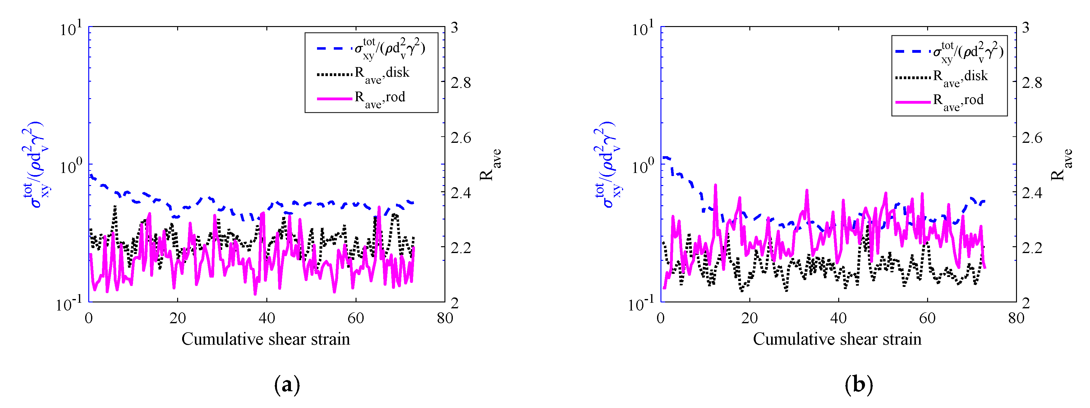
Shear flows of binary mixtures of rods and disks, which have the same particle volume, are simulated to examine the effect of particle shape difference on the stacking and ordering behavior. Figure 7 shows the evolution of normalized shear stress and average stack size with cumulative shear strain for binary mixture flows with various rods fractions . In the binary mixtures, rods and disks have aspect ratios of AR = 6 and AR = 0.3, respectively, and the solid volume fraction is set to ν = 0.5. A stack is formed by particles of the same shape, as shown in Figure 4b. Thus, the stack sizes are measured for the rods and disks separately. As shown in Figure 7a, for a binary mixture with C = 0.25, the average shear stress initially decreases and then approaches a steady-state value. The average stack sizes, which are the same for the rods and disks, remain constant in the flow process. As the rods fraction C increases (Figure 7b,c), an initial decrease in the shear stress is also obtained; however, a larger magnitude of the stress decrease is observed. The average stack size of the disks with AR = 0.3 still remains constant, while the average stack size of the rods with AR = 6 shows a slight increase with the cumulative shear strain.
The variation of normalized shear stress and fraction of stacking particles P with cumulative shear strain is plotted in Figure 8 for the binary mixture flows with various rods fractions C. The fraction of stacking particles is calculated for each particle species
where is the number of particles of species i that are included in the stacks and is the total number of particles of species i in the mixture. It can be seen from Figure 8 that as the rods fraction increases, the fraction of stacking rods with AR = 6 increases and the fraction of stacking disks with AR = 0.3 decreases. Thus, the concentration of a particle species can promote stacking of that species.
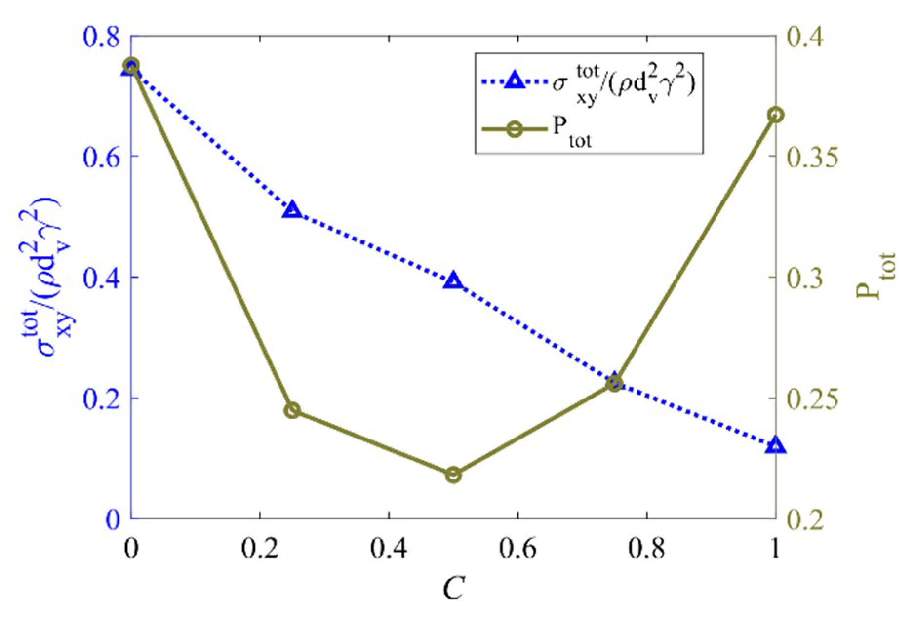
For a binary mixture, Equation (17) can be used to calculate the overall fraction of stacking particles , in which is the total number of particles (including rods and disks) in the stacks and is the total number of all the particles in the mixture. The average normalized shear stress and the average value of at the flow’s steady state are plotted as a function of rods fraction C in Figure 9. The rods fraction C = 0 corresponds to monodisperse disk flow and C = 1 corresponds to monodisperse rod flow. Figure 9 shows that the shear stress decreases monotonically with an increase of C, while the overall fraction of stacking particles shows a U-shape dependence on C. A stack of particles is a structure with geometric tessellation and mechanical stability. The face-on-face stacking of disks and band-on-band stacking of rods can achieve such compacted tessellation with good mechanical stability. In binary mixtures, due to the interaction between the particles of different shapes (i.e., disks and rods), stacking is interrupted. As a result, the overall fractions of stacking particles for binary mixtures are smaller than those of monodisperse rods and disks. The worst stacking occurs in the well-mixed binary mixture with 50% rods and 50% disks (i.e., C = 0.5).
Evolution of the normalized shear stress and order parameter S with cumulative shear strain is plotted in Figure 10 for binary mixture flows with various rods fractions. In Figure 10, the order parameter S is calculated for each particle species in the mixture. At the early stage of the flow process, as the stress declines, the order parameter S for the rods increases. The stress and order parameter reach steady state at the same cumulative shear strain. This observation is consistent with that of the monodisperse rod flow (see Figure 6f). The order parameter S for the disks fluctuates between 0.5 and 0.6 in the flow process, which is similar to the observation of monodisperse disk flow (see Figure 6e).
In a binary mixture, given the order parameter of rods and order parameter of disks , a volume-averaged order parameter Save can be defined to quantify the degree of particle alignment for the whole mixture
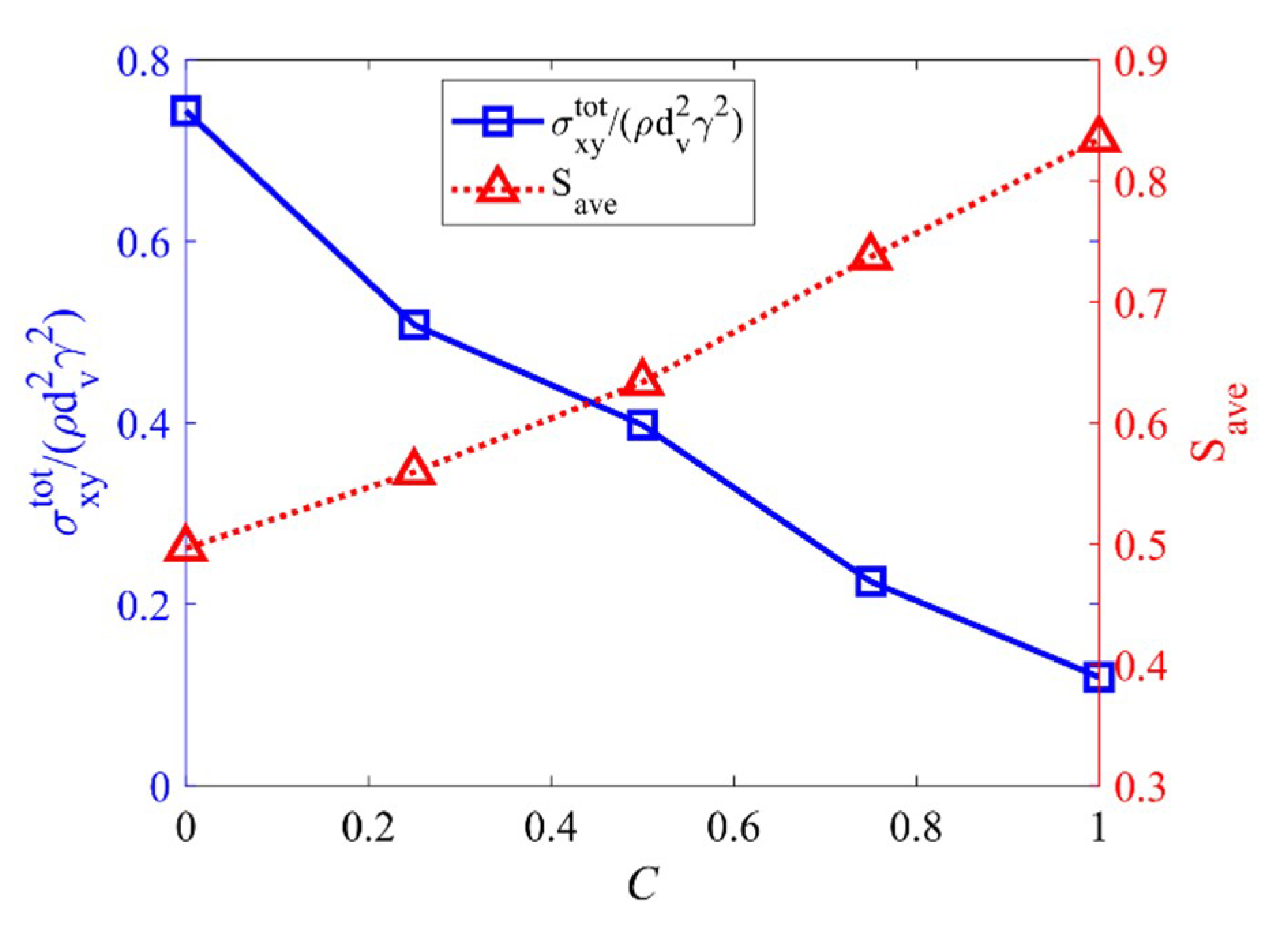
The average normalized shear stress and the average order parameter are plotted in Figure 11 as a function of rods fraction C for the binary mixtures. The stress declines monotonically with increasing C and the order parameter increases monotonically with increasing C. This indicates that the stress decreases as the order parameter increases. The correlation between the system stresses and order parameter is further discussed in the following sections.
4. Effect of Particle Shape Polydispersity on Stresses
Different binary mixtures with the same rods (AR = 6) but different disks have been modeled. Disks of AR = 0.3, 0.2, 0.15 and 0.1 (the smaller AR corresponds to the flatter disks) have been considered in this work. Average normalized shear stress at steady state is plotted as a function of solid volume fraction for various binary mixtures in Figure 12. In general, the stress curves of binary mixtures exhibit a W-shape, similar to those of monodisperse cylindrical particle flows [30]. For binary mixtures of AR = 0.3 and AR = 6 (Figure 12a), the stresses of the mixtures (with ) are bounded by those of the two monodisperse flows (with and ). When the disks become flatter by reducing the AR, as shown in Figure 12b–d, the stresses of the mixtures are sandwiched between those of the two monodisperse systems at low solid volume fractions ( < 0.4). Nevertheless, it is interesting to observe that the stresses of the mixtures can be larger than the stresses of both corresponding monodisperse systems at large solid volume fractions ( > 0.4).
For a clearer comparison between the stresses of binary and monodisperse systems, the average normalized shear stresses are plotted as a function of rods fraction C in Figure 13. The stresses show a monotonic change with rods fraction at each solid volume fraction considered for the mixtures of AR = 0.3 and AR = 6 (Figure 13a). For the mixtures of AR = 0.2 and AR = 6 (Figure 13b), the stress decreases monotonically with increasing C when ≤ 0.4 and the stress curve exhibits a hump shape when = 0.5, demonstrating that the stresses of the mixtures can be greater than those of the monodisperse systems. For the mixtures of AR = 0.15 and AR = 6 (Figure 13c), the stress is independent of rods fraction C at solid volume fractions of ≤ 0.4, due to the fact that two monodisperse flows (C = 0 and 1) have the same stress. The humped stress curves are observed when the solid volume fraction is > 0.4, and the stress difference between the mixtures and monodisperse systems increases as increases. For the mixtures of AR = 0.1 and AR = 6 (Figure 13d), the stress increases monotonically with increasing C when ≤ 0.4, because the stress of monodisperse rods (C = 1) is larger than that of the monodisperse disks (C = 0). The humped stress curve occurs when = 0.5.
As discussed previously, the results of Figure 13 show that increased particle shape difference and increased solid volume fraction lead to larger stresses for the binary mixtures when compared to the monodisperse systems. It is presumed that the large particle shape difference makes the particles more difficultly tessellate in a confined space for the dense flows, thus promoting particle–particle interaction. As a result, larger stresses are obtained for the mixtures than for the monodisperse systems. Evidence for the enhanced particle–particle interaction is provided by considering the particle rotational kinetic energies. As shown in Figure 14a, the average rotational kinetic energy of particles generally decreases with increasing rods fraction for the binary mixtures of AR = 0.3 and 6 at the solid volume fraction ν = 0.5. This trend is consistent with the variation of the stress with , as shown in Figure 13a. For the binary mixtures of AR = 0.15 and 6 at ν = 0.55, larger average rotational kinetic energies of particles are obtained for the mixtures (Figure 14b), and consistently larger stresses are obtained for these mixtures (Figure 13c). Thus, larger stresses of the mixtures are caused by the enhanced particle–particle interaction, resulting in larger particle rotational kinetic energies. The present simulation results also show that the average translational particle kinetic energy is independent of the rods fraction (not shown here) and therefore, the translational motion of particles is mainly determined by the assigned mean flow field. In addition, for the binary mixtures of AR = 0.15 and 6 at ν = 0.55, smaller average order parameters are observed compared to those of the monodisperse flows, as shown in Figure 15. The reduction in the order parameters , i.e., the degree of particle alignment, is consistent with the enhanced particle rotation (Figure 14b).
5. Correlation between Stresses and Order Parameter
As discussed in the previous sections, the particle-phase stresses exhibit a strong dependence on the order parameter in dense granular flows ( ≥ 0.4). In the shear flow simulations of monodispersed cylindrical particle flows by Berzi et al. [36], they found that the viscosity, i.e., the ratio of shear stress to shear rate, was strongly dependent on the order parameter at large solid volume fractions, for which particle alignment was significant. In this section, the correlation between the particle-phase stresses and the order parameter for binary mixtures is discussed.
Different binary mixtures of different combinations of particle aspect ratios (AR = 0.1 and 6, AR = 0.15 and 6, AR = 0.2 and 6, and AR = 0.3 and 6) with different rods fractions (C = 0.25, 0.5, and 0.75) are modeled in the present simulations. Variations of the normalized shear stress, normalized pressure, and ratio of shear stress to pressure with average order parameter is plotted in Figure 16 for various binary mixtures at a solid volume fraction of = 0.5. The pressure is the average value of three normal stress components, i.e., . As shown in Figure 16a,b, the data for shear stresses and pressures collapse on master curves, especially for > 0.5. Some scattering data are observed at smaller order parameters. These results indicate that the particle-phase stresses have a strong dependence on the order parameter when the particle alignment becomes significant with > 0.5, regardless of particle aspect ratios and compositions of the binary mixtures; While the particle shape and the composition of a mixture also play a role in determining the stresses of a randomly oriented particle bed with a small order parameter. In dense flows, the collisional stress component determines the total stress [30]. The collisional stress depends on the particle–particle contact forces (see Equation (11)). The alignment of particles can reduce the projected area of a particle in the plane perpendicular to the flow, reducing the interference of neighboring particles and thus decreasing the particle–particle contact forces. As a result, the particle alignment-dependence of the particle–particle contact forces may lead to the order parameter-dependence of the particle phase stresses. Since the shear stresses and pressures are functions of the order parameter , their ratio, which is known as the bulk friction coefficient, also depends on , as shown in Figure 16c.
The normalized shear stress and pressure are assumed to follow the exponential correlations,
The coefficients and can be determined by fitting to the data in Figure 16a, and and can be determined by fitting to the data in Figure 16b. The values of , , , and are provided in Table 2. Dividing Equation (21) by Equation (22) gives,
The curve on Figure 16c represents Equation (23).
The solid volume fraction also has a significant impact on the stresses. Figure 17 shows the variation of normalized shear stress, normalized pressure, and ratio of shear stress to pressure with average order parameter at various solid volume fractions. The binary mixtures consist of the disks with AR = 0.15 and the rods with AR = 6. It can be seen that different exponential expressions with different sets of coefficients (, , , and ) can be determined for the different solid volume fractions. Thus, the four coefficients, , , , and , can be expressed as functions of solid volume fraction , and polynomial functions are assumed as follows,
By fitting to the obtained data, the coefficients in Equation (24) can be determined for , , , and , as presented in Table 3.
Equation (23) can be rewritten as,
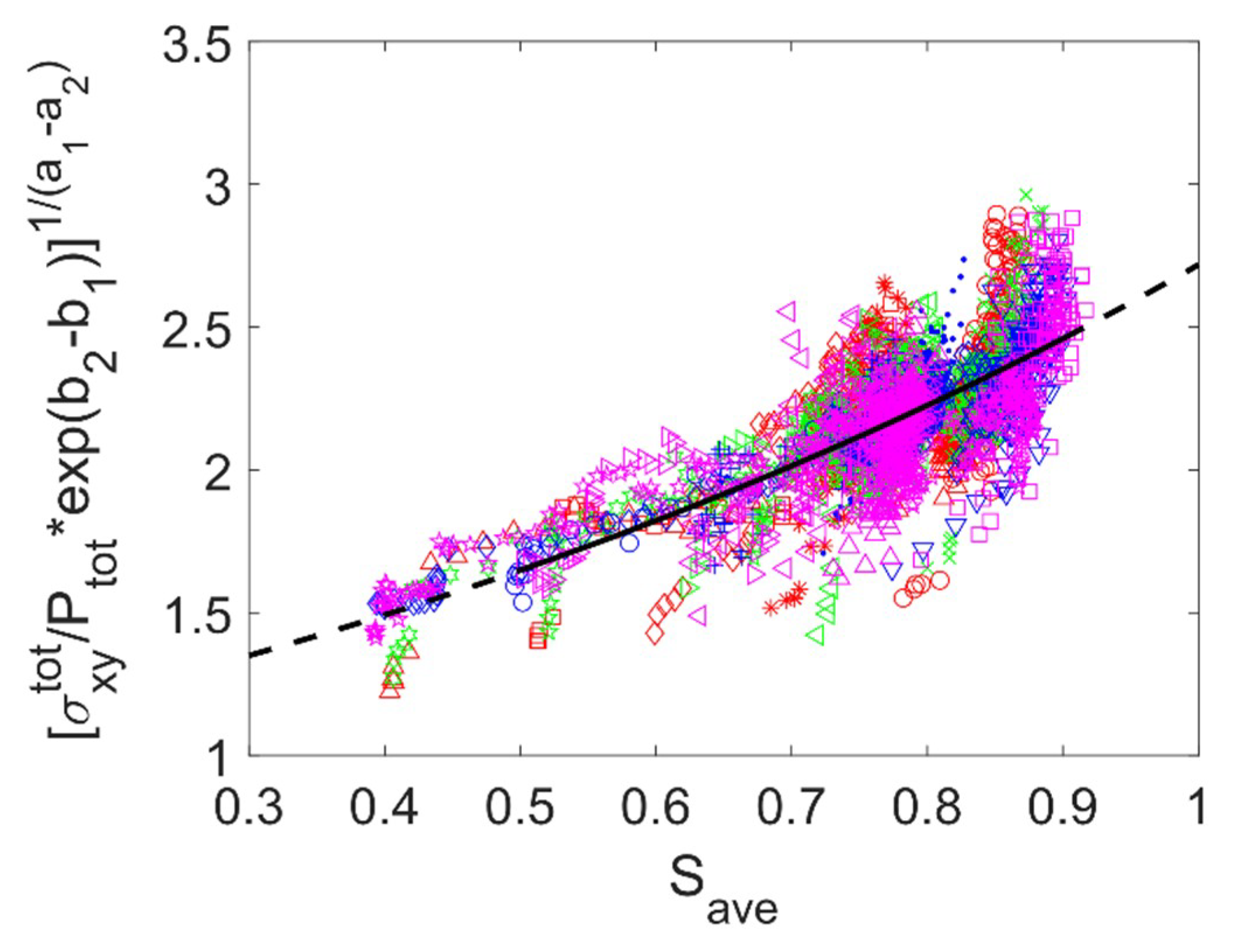
The term on the left-hand side of the above equation is the bulk friction coefficient modified by the parameters which can be expressed as functions of the solid volume fraction ν (Equation (24)). The modified bulk friction coefficient is plotted against the order parameter in Figure 18. The data for the various binary mixtures, which are presented in Figure 17c, tend to collapse on an exponential curve in Figure 18. The effects of particle alignment, compositions of the mixtures, and solid volume fractions on the bulk friction coefficient have been considered in the empirical correlation shown in Figure 18. It should be noted that the results presented in Figure 16, Figure 17 and Figure 18 include not only the steady-state data, but also the data before the steady flow is achieved, illustrating the strong order parameter-dependence of the stresses.
6. Conclusion
Granular shear flows of binary mixtures of frictionless rods and disks are simulated using the Discrete Element Method (DEM). In the binary mixtures, rods and disks have the same volume but significantly different shapes. Thus, the effects of particle shape differences on the binary mixture flows are investigated in this work. In shear flows, the rods and disks show stacking and ordering behavior, which is enhanced as the flow develops before reaching a steady state. By changing the rods fraction in the mixture, the average stack size changes slightly. The number fraction of the particles that are included in the stacks is smaller for the binary mixtures than for the monodisperse rods or disks, because the probability to form a stacking structure is reduced by the contacts between the particles of different shapes.
A summary of the main results and conclusions on the stresses of the binary mixtures of rods and disks are presented as follows:
- ♦
- For the binary mixtures of the rods with AR = 6 and the disks with AR = 0.3, the stresses of the mixtures are bounded between the stresses of the monodisperse rods (AR = 6) and the monodisperse disks (AR = 0.3). At a given solid volume fraction, as the rods fraction increases from 0 to 1, the stress of the mixture changes monotonically from the stress of the monodisperse disks (AR = 0.3) to the stress of the monodisperse rods (AR = 6).
- ♦
- For the binary mixtures of the rods with AR = 6 and the disks with AR = 0.2, 0.15 and 0.1, the stresses of the mixtures are still bounded by the stresses of corresponding monodisperse systems at the low solid volume fractions ( < 0.4), while larger stresses are obtained for the mixtures than for the monodisperse systems at the high solid volume fractions ( ≥ 0.4). It is found that the average particle rotational kinetic energies of these mixtures are greater than those of the monodisperse rods and disks in the dense flows, because larger difference in particle shape causes difficulties for the dense packing, leading to stronger particle–particle interaction in the flow. Due to the enhanced particle rotation, smaller order parameters, which is a measure of the degree of particle alignment, are obtained for the mixtures than the monodisperse systems.
- ♦
- The data of the stresses versus the order parameter for dense binary flows with different particle shapes and different compositions can collapse on exponential function curves, indicating the strong dependence of the stresses on the particle alignment. Based on the simulation results, an empirical expression of bulk friction coefficient (ratio of the shear stress to pressure) for the dense binary flows is proposed to account for the effects of the particle alignment and solid volume fraction.
- ♦
- The previous dense granular flow models, such as the -theory [4], have been successfully applied to the spherical particle flows. However, the effect of particle shape is difficult to be taken into account in these models. The present results (Equations (21)–(25)) may give a hint that the order parameter S should be included in the rheological laws for the elongated and flat particle flows.
Author Contributions
Investigation and Validation, Y.L., Z.Y., J.Y.; Methodology and Software, C.W., J.S.C., Y.G.; Formal Analysis, All authors; Writing—Original draft preparation, Y.L.; Writing—Review & Editing, Y.G., C.W., J.S.C.; Funding Acquisition, Y.G. All authors have read and agreed to the published version of the manuscript.
Funding
The National Natural Science Foundation of China (Grant 11872333 and 91852205) and the Zhejiang Provincial Natural Science Foundation of China (Grant LR19A020001) are acknowledged for the financial supports.
Conflicts of Interest
The authors declare no conflict of interest.
Appendix A

Table A1.
Determination of overlap size, contact normal vector, and contact point position for the basic contact types between two cylindrical particles. The equations, which can be found in [24], are defined in particle i’s body-fixed frame of reference. The contact detection algorithms for several special contact scenarios are referred to [25].
| Contact Types | Equations |
|---|---|
Face–face contact | Overlap size: = (Li + Lj)/2 where Li and Lj are the major axial lengths of contacting cylinders i and j, is the z-coordinate of the center of particle j in particle i’s body-fixed frame of reference. Contact normal vector: = [0, 0, sign ()] in which the function ‘sign’ returns the sign of the expression. Contact point position: , in which, (Ri ), , , where and are the radii, respectively, of the particles i and j, and and are the x and y-coordinates, respectively, of the center of the particle j. |
Face–band contact | Overlap size: Li/2 + Rj. Contact normal vector: = sign () in which is the unit vector along z-axis of the particle i in the particle i’s body-fixed frame of reference. Contact point position: ()(0,0,1)i where and are the position vectors of the point A and B, respectively, in the particle i’s body-fixed frame of reference. |
Face–edge contact | Overlap size: Li/2 in which is the z-coordinate of the point E in the particle i’s body-fixed frame of reference. Contact normal vector: = sign () where is the unit vector along z-axis in the particle i’s frame of reference. Contact point position: + )()(0,0,1)i In which is the position of the point E in the particle i’s body-fixed frame of reference. |
Parallel band–band contact | Overlap size: Ri + Rj Contact normal vector: Contact point position: in which, (Ri) |
Skewed band–band contact | Overlap size: (Ri + Rj)-d where d is the shortest distance between the two axes of contacting cylindrical particles. Contact normal vector: where and are the positions of the intersection points of the shortest distance line with the major axes of the particle i and the particle j, respectively. Contact point position: |
Band–edge contact | Overlap size: Ri in which and are the x and y coordinates of the point E, which is on the edge of the particle j and has the shortest distance to the major axis of the particle i. Contact normal vector: Contact point position: |
Edge–edge contact | Overlap size: The overlap size is equal to the shortest distance between AB and CD, in which, , and is the position of the center of CD, and is the position of the center of AB. Contact normal vector: Contact point position: |
References
- Lun, C.K.K.; Savage, S.B.; Jeffrey, D.J.; Chepurniy, N. Kinetic theories for granular flow: Inelastic particles in Couette flow and slightly inelastic particles in a general flow field. J. Fluid Mech. 1984, 140, 223–256. [Google Scholar] [CrossRef]
- Chialvo, S.; Sundaresan, S. A modified kinetic theory for frictional granular flows in dense and dilute regimes. Phys. Fluids. 2013, 25, 070603. [Google Scholar] [CrossRef] [Green Version]
- Berzi, D.; Vescovi, D. Different singularities in the functions of extended kinetic theory at the origin of the yield stress in granular flows. Phys. Fluids. 2015, 27, 013302. [Google Scholar] [CrossRef]
- Jop, P.; Forterre, Y.; Pouliquen, O. A constitutive law for dense granular flows. NATURE 2006, 441, 727–730. [Google Scholar] [CrossRef] [Green Version]
- Kamrin, K.; Koval, G. Nonlocal Constitutive Relation for Steady Granular Flow. Phys. Rev. Lett. 2012, 108, 178301. [Google Scholar] [CrossRef] [PubMed]
- Bouzid, M.; Trulsson, M.; Claudin, P.; Clement, E.; Andreotti, B. Nonlocal Rheology of Granular Flows Across Yield Conditions. Phys. Rev. Lett. 2013, 111, 238301. [Google Scholar] [CrossRef] [PubMed] [Green Version]
- Pähtz, T.; Orencio, D.; de Klerk, D.N.; Govender, I.; Trulsson, M. Local Rheology Relation with Variable Yield Stress Ratio across Dry, Wet, Dense, and Dilute Granular Flows. Phys. Rev. Lett. 2019, 123, 048001. [Google Scholar] [CrossRef] [PubMed] [Green Version]
- Shen, H.H. Stresses in a rapid flow of spherical solid with two sizes. Particul. Sci. Technol. 1984, 2, 37–56. [Google Scholar] [CrossRef]
- Jenkins, J.T.; Mancini, F. Balance Laws and Constitutive Relations for Plane Flows of a Dense, Binary Mixture of Smooth, Nearly Elastic, Circular Disks. J. Appl. Mech. 1987, 54, 27–34. [Google Scholar] [CrossRef]
- Farrell, M.; Lun, C.K.K.; Savage, S.B. A simple kinetic theory for granular flow of binary mixtures of smooth, inelastic, spherical particles. Acta Mech. 1986, 63, 45–60. [Google Scholar] [CrossRef]
- Van Beijeren, H.; Ernst, M.H. The modified Enskog equation. Physica 1973, 68, 437–456. [Google Scholar] [CrossRef]
- Willits, J.T.; Arnarson, B.O. Kinetic theory of a binary mixture of nearly elastic disks. Phys. Fluids 1999, 11, 3116. [Google Scholar] [CrossRef]
- Clelland, R.; Hrenya, C.M. Simulations of a Binary-Sized Mixture of Inelastic Grains in Rapid Shear Flow. Phys. Rev. E 2002, 65, 031301. [Google Scholar] [CrossRef] [PubMed]
- Galvin, J.E.; Dahl, S.R.; Hrenya, C.M. On the role of non-equipartition in the dynamics of rapidly flowing granular mixtures. J. Fluid Mech. 2004, 528, 207–232. [Google Scholar] [CrossRef]
- Iddir, H.; Arastoopour, H. Modeling of multitype particle flow using the kinetic theory approach. Aiche J. 2005, 51, 1620–1632. [Google Scholar] [CrossRef]
- Benyahia, S. Verification and validation study of some polydisperse kinetic theories. Chem. Eng. Sci. 2008, 63, 5672–5680. [Google Scholar] [CrossRef]
- Tripathi, A.; Khakhar, D.V. Rheology of binary granular mixtures in the dense flow regime. Phys. Fluids 2011, 23, 113302. [Google Scholar] [CrossRef]
- Gu, Y.; Ozel, A.; Sundaresan, S. Rheology of granular materials with size distributions across dense-flow regimes. Powder Technol. 2016, 295, 322–329. [Google Scholar] [CrossRef]
- Dahl, S.R.; Clelland, R.; Hrenya, C.M. The effects of continuous size distributions on the rapid flow of inelastic particles. Phys. Fluids. 2002, 14, 1972–1984. [Google Scholar] [CrossRef]
- Dahl, S.R.; Clelland, R.; Hrenya, C.M. Three-dimensional, rapid shear flow of particles with continuous size distributions. Powder Technol. 2003, 138, 7–12. [Google Scholar] [CrossRef]
- Yang, J.; Guo, Y.; Buettner, K.E.; Curtis, J.S. DEM investigation of shear flows of binary mixtures of non-spherical particles. Chem. Eng. Sci. 2019, 202, 383–391. [Google Scholar] [CrossRef]
- Hao, J.H.; Li, Y.J.; Guo, Y.; Jin, H.H.; Curtis, J.S. The effect of polydispersity on the stresses of cylindrical particle flows. Powder Technol. 2019, 361, 14876. [Google Scholar] [CrossRef]
- Cundall, P.A.; Strack, O.D.L. A discrete numerical model for granular assemblies. Geotechnique 1980, 30, 331–336. [Google Scholar] [CrossRef] [Green Version]
- Kodam, M.; Bharadwaj, R.; Curtis, J.; Hancock, B.; Wassgren, C. Cylindrical object contact detection for use in discrete element method simulations. Part I—Contact detection algorithms. Chem. Eng. Sci. 2010, 65, 5852–5862. [Google Scholar] [CrossRef]
- Guo, Y.; Wassgren, C.; Ketterhagen, W.; Hancock, B.; Curtis, J. Some computational considerations associated with discrete element modeling of cylindrical particles. Powder Technol. 2012, 228, 193–198. [Google Scholar] [CrossRef]
- Baraff, D. Rigid body simulation. Physically Based Modeling (SIGGRAPH Course Notes). 2001, pp. G1–G68. Available online: www.cs.cmu.edu/~baraff/sigcourse/notesd1.pdf (accessed on 2 February 2020).
- Hertz, H. Uber die Ber “uhrung fester elastischer K” orper. Reine Angew. 1882, 92, 156–171. [Google Scholar]
- Tangri, H.; Guo, Y.; Curtis, J.S. Packing of cylindrical particles: DEM simulations and experimental measurements. Powder Technol. 2017, 317, 72–82. [Google Scholar] [CrossRef]
- Tangri, H.; Guo, Y.; Curtis, J.S. Hopper Discharge of Elongated Particles of Varying Aspect Ratio: Experiments and DEM simulations. Chem. Eng. Sci. 2019, 4, 100040. [Google Scholar] [CrossRef]
- Guo, Y.; Wassgren, C.; Ketterhagen, W.; Hancock, B.; James, B.; Curtis, J. A numerical study of granular shear flows of rod-like particles using the discrete element method. J. Fluid Mech. 2012, 713, 1–26. [Google Scholar] [CrossRef]
- Azéma, E.; Estrada, N.; Preechawuttipong, I.; Delenne, J.; Radjai, F. Systematic description of the effect of particle shape on the strength properties of granular media. EPJ Web Conf. 2017, 140, 06026. [Google Scholar] [CrossRef] [Green Version]
- Lees, A.W.; Edwards, S.F. The computer study of transport processes under extreme conditions. J. Phys. C Solid State Phys. 1972, 5, 1921–1928. [Google Scholar] [CrossRef]
- Kafui, K.D.; Thornton, C.; Adams, M.J. Discrete particle-continuum fluid modelling of gas–solid fluidised beds. Chem. Eng. Sci. 2002, 57, 2395–2410. [Google Scholar] [CrossRef]
- Börzsönyi, T.; Szabó, B.; Törös, G.; Wegner, S.; Török, J.; Somfai, E.; Bien, T.; Stannarius, R. Orientational Order and Alignment of Elongated Particles Induced by Shear. Phys. Rev. Lett. 2012, 108, 228302. [Google Scholar] [CrossRef] [PubMed] [Green Version]
- Wegner, S.; Börzsönyi, T.; Bien, T.; Rose, G.; Stannarius, R. Alignment and dynamics of elongated cylinders under shear. Soft Matter 2012, 8, 10950. [Google Scholar] [CrossRef]
- Berzi, D.; Thai-Quang, N.; Guo, Y.; Curtis, J. Stresses and orientational order in shearing flows of granular liquid crystals. Phys. Rev. E 2016, 93, 040901. [Google Scholar] [CrossRef] [Green Version]
Figure 1.
Geometries of (a) a rod and (b) a disk modeled in the present DEM simulations.

Figure 2.
Numerical model of shear flow of a binary mixture of rods and disks.

Figure 3.
Evolution of normalized shear stress for (a) the binary mixture of AR = 0.3 and AR = 6 at the solid volume fraction = 0.4 with different time steps and (b) the binary mixture of AR = 0.3 and AR = 6 at = 0.05 with different shear domain sizes. Rods fraction is C = 0.5 for the two mixtures.
Figure 3.
Evolution of normalized shear stress for (a) the binary mixture of AR = 0.3 and AR = 6 at the solid volume fraction = 0.4 with different time steps and (b) the binary mixture of AR = 0.3 and AR = 6 at = 0.05 with different shear domain sizes. Rods fraction is C = 0.5 for the two mixtures.

Figure 4.
(a) An illustration of the criterion to determine a stacking structure, and (b) formation of stackings in a shear flow of a binary mixture of rods (AR = 6) and disks (AR = 0.3). The non-stacking particles are removed from the image (b).
Figure 4.
(a) An illustration of the criterion to determine a stacking structure, and (b) formation of stackings in a shear flow of a binary mixture of rods (AR = 6) and disks (AR = 0.3). The non-stacking particles are removed from the image (b).

Figure 5.
Stacking of (a) disks (AR = 0.3) and (b) rods (AR = 6) in monodisperse flows at solid volume fraction ν = 0.5. Particles that are not part of stacks are omitted in the figures.
Figure 5.
Stacking of (a) disks (AR = 0.3) and (b) rods (AR = 6) in monodisperse flows at solid volume fraction ν = 0.5. Particles that are not part of stacks are omitted in the figures.

Figure 6.
Evolution of normalized shear stress, average stack size (first row), fraction of stacking particles P (second row), and order parameter S (third row) with cumulative shear strain for the monodisperse shear flows with disks of AR = 0.3 (first column) and rods of AR = 6 (second column): (a) Rave versus cumulative shear strain for AR = 0.3, (b) Rave versus cumulative shear strain for AR = 6, (c) P versus cumulative shear strain for AR = 0.3, (d) P versus cumulative shear strain for AR = 6, (e) S versus cumulative shear strain for AR = 0.3, (f) S versus cumulative shear strain for AR = 6. The solid volume fraction is ν = 0.5.


Figure 7.
Evolution of normalized shear stress and average stack size with cumulative shear strain for binary mixture flows of AR = 0.3 (disks) and AR = 6 (rods) with a rods fraction (a) C = 0.25, (b) C = 0.5, and (c) C = 0.75. The solid volume fraction is ν = 0.5.
Figure 7.
Evolution of normalized shear stress and average stack size with cumulative shear strain for binary mixture flows of AR = 0.3 (disks) and AR = 6 (rods) with a rods fraction (a) C = 0.25, (b) C = 0.5, and (c) C = 0.75. The solid volume fraction is ν = 0.5.


Figure 8.
Evolution of normalized shear stress and fraction of stacking particles P with cumulative shear strain for binary mixture flows of AR = 0.3 (disks) and AR = 6 (rods) with (a) C = 0.25, (b) C = 0.5, and (c) C = 0.75. The solid volume fraction is ν = 0.5.
Figure 8.
Evolution of normalized shear stress and fraction of stacking particles P with cumulative shear strain for binary mixture flows of AR = 0.3 (disks) and AR = 6 (rods) with (a) C = 0.25, (b) C = 0.5, and (c) C = 0.75. The solid volume fraction is ν = 0.5.

Figure 9.
Variation of the average normalized shear stress and the overall fraction of stacking particles with the rods fraction C for binary mixtures of AR = 0.3 and AR = 6. The solid volume fraction is ν = 0.5.
Figure 9.
Variation of the average normalized shear stress and the overall fraction of stacking particles with the rods fraction C for binary mixtures of AR = 0.3 and AR = 6. The solid volume fraction is ν = 0.5.

Figure 10.
Evolution of normalized shear stress and order parameter S with cumulative shear strain for binary mixture flows of AR = 0.3 (disks) and AR = 6 (rods) with rods fractions (a) C = 0.25, (b) C = 0.5, and (c) C = 0.75. The solid volume fraction is ν = 0.5.
Figure 10.
Evolution of normalized shear stress and order parameter S with cumulative shear strain for binary mixture flows of AR = 0.3 (disks) and AR = 6 (rods) with rods fractions (a) C = 0.25, (b) C = 0.5, and (c) C = 0.75. The solid volume fraction is ν = 0.5.

Figure 11.
The average normalized shear stress and the average order parameter as a function of rods fraction C for binary mixtures of AR = 0.3 and AR = 6, solid volume fraction ν = 0.5.
Figure 11.
The average normalized shear stress and the average order parameter as a function of rods fraction C for binary mixtures of AR = 0.3 and AR = 6, solid volume fraction ν = 0.5.

Figure 12.
Average normalized shear stresses at the steady state for various binary mixtures with (a) AR = 0.3 and AR = 6, (b) AR = 0.2 and AR = 6, (c) AR = 0.15 and AR = 6, and (d) AR = 0.1 and AR = 6. An error bar represents the standard deviation of the stress from the average value at steady state.

Figure 13.
Variation of average normalized shear stress with rods fraction C for moderate and dense flows of the binary mixtures with (a) AR = 0.3 and AR = 6, (b) AR = 0.2 and AR = 6, (c) AR = 0.15 and AR = 6, and (d) AR = 0.1 and AR = 6. An error bar represents the standard deviation of the stresses from the average value at steady state.

Figure 14.
Average rotational kinetic energy of particles as a function of rods fraction C for the binary mixtures of (a) AR = 0.3 and 6, ν = 0.5 and (b) AR = 0.15 and 6, ν = 0.55. An error bar represents the standard deviation of particle rotational kinetic energies from the average value at the steady flow state.

Figure 15.
The average normalized shear stress and the average order parameter as a function of rods fraction C for the binary mixtures of AR = 0.15 and AR = 6. The solid volume fraction is ν = 0.55.
Figure 15.
The average normalized shear stress and the average order parameter as a function of rods fraction C for the binary mixtures of AR = 0.15 and AR = 6. The solid volume fraction is ν = 0.55.

Figure 16.
Variation of (a) normalized shear stress, (b) normalized pressure, and (c) ratio of shear stress to pressure with average order parameter for various binary mixtures. The solid volume fraction is ν = 0.5.
Figure 16.
Variation of (a) normalized shear stress, (b) normalized pressure, and (c) ratio of shear stress to pressure with average order parameter for various binary mixtures. The solid volume fraction is ν = 0.5.


Figure 17.
Variation of (a) normalized shear stress, (b) normalized pressure, and (c) ratio of shear stress to pressure with average order parameter for the binary mixtures (AR = 0.15 and AR = 6) at various solid volume fractions . It is noted that the vertical coordinate is the logarithmic coordinate. Thus, the stresses have the exponential dependence on for various .


Figure 18.
Collapse of the ratios of shear stress to pressure for binary mixtures (AR = 0.15 and AR = 6) with various rods fractions C and solid volume fractions ν. The legend of symbols in Figure 17a is also applied in this figure.
Figure 18.
Collapse of the ratios of shear stress to pressure for binary mixtures (AR = 0.15 and AR = 6) with various rods fractions C and solid volume fractions ν. The legend of symbols in Figure 17a is also applied in this figure.

Table 1.
Particle properties and simulation parameters.
| AR | dv (m) | ρ (kg/m3) | E (Pa) | ζ | γ (s−1) | |
|---|---|---|---|---|---|---|
| 0.1, 0.15, 0.2, 0.3, and 6 | 2.38 × 10⁻⁴ | 2500 | 8.7 × 10⁹ | 0.3 | 0.9 | 100 |
Table 2.
Coefficients in Equations (21) and (22) for binary flows at the solid volume fraction of ν = 0.5.
Table 2.
Coefficients in Equations (21) and (22) for binary flows at the solid volume fraction of ν = 0.5.
| Coefficients | ||||
|---|---|---|---|---|
| Values | −5.0174 | 2.2389 | −3.3785 | 2.8122 |
Table 3.
Coefficients in Equation (24).
| 3235.0 | −4730.0 | 2258.6 | −356.60 | |
| 2243.7 | −3343.9 | 1617.2 | −257.18 | |
| −2439.4 | 3610.5 | −1731.9 | 270.80 | |
| −1643.9 | 2506.1 | −1222.6 | 193.67 |
© 2020 by the authors. Licensee MDPI, Basel, Switzerland. This article is an open access article distributed under the terms and conditions of the Creative Commons Attribution (CC BY) license (http://creativecommons.org/licenses/by/4.0/).
Share and Cite
MDPI and ACS Style
Liu, Y.; Yu, Z.; Yang, J.; Wassgren, C.; Curtis, J.S.; Guo, Y. Discrete Element Method Investigation of Binary Granular Flows with Different Particle Shapes. Energies 2020, 13, 1841. https://0-doi-org.brum.beds.ac.uk/10.3390/en13071841
AMA Style
Liu Y, Yu Z, Yang J, Wassgren C, Curtis JS, Guo Y. Discrete Element Method Investigation of Binary Granular Flows with Different Particle Shapes. Energies. 2020; 13(7):1841. https://0-doi-org.brum.beds.ac.uk/10.3390/en13071841
Chicago/Turabian StyleLiu, Yi, Zhaosheng Yu, Jiecheng Yang, Carl Wassgren, Jennifer Sinclair Curtis, and Yu Guo. 2020. "Discrete Element Method Investigation of Binary Granular Flows with Different Particle Shapes" Energies 13, no. 7: 1841. https://0-doi-org.brum.beds.ac.uk/10.3390/en13071841
Note that from the first issue of 2016, this journal uses article numbers instead of page numbers. See further details here.