A Fractal Discrete Fracture Network Based Model for Gas Production from Fractured Shale Reservoirs

Abstract

A fractal discrete fracture network based model was proposed for the gas production prediction from a fractured shale reservoir. Firstly, this model was established based on the fractal distribution of fracture length and a fractal permeability model of shale matrix which coupled the multiple flow mechanisms of slip flow, Knudsen diffusion, surface diffusion, and multilayer adsorption. Then, a numerical model was formulated with the governing equations of gas transport in both a shale matrix and fracture network system and the deformation equation of the fractured shale reservoir. Thirdly, this numerical model was solved within the platform of COMSOL Multiphysics (a finite element software) and verified through three fractal discrete fracture networks and the field data of gas production from two shale wells. Finally, the sensitivity analysis was conducted on fracture length fractal dimension, pore size distribution, and fracture permeability. This study found that cumulative gas production increases up to 113% when the fracture fractal length dimension increases from 1.5 to the critical value of 1.7. The gas production rate declines more rapidly for a larger fractal dimension (up to 1.7). Wider distribution of pore sizes (either bigger maximum pore size or smaller minimum pore size or both) can increase the matrix permeability and is beneficial to cumulative gas production. A linear relationship is observed between the fracture permeability and the cumulative gas production. Thus, the fracture permeability can significantly impact shale gas production.

1. Introduction

Horizontal well drilling and hydraulic fracturing are two key technologies to the economic production of unconventional oil and gas reservoirs [1,2]. Hydraulic fracturing can create a complex fracture network in unconventional shale oil or gas reservoirs for significant enhancement of oil or gas production. Therefore, more attentions should be paid to the gas flow in a complex fracture network [3,4,5]. However, an accurate and efficient numerical simulation model for a fractured shale reservoir is still a challenge.

Complex gas transport mechanisms and fracture networks may interact in a fractured fractal gas reservoir. The complex gas transport mechanisms include the slip flow, Knudsen diffusion, multilayer adsorption/desorption, surface diffusion, and adsorbed gas porosity. These flows occur in nanopores and organic matter of shale matrix [4,6,7,8,9,10]. Many permeability models have been proposed to consider the gas transport mechanisms and the distinct fractal characteristics of pore size distribution in shale matrix [11,12,13,14]. However, they did not consider the impacts of a fractal fracture network in fractured shale gas reservoirs.

Shale formation has many fractures in both microscopic and field scales [15,16,17,18]. These fractures form a discrete fracture network and govern the permeability of the fractured shale reservoir. In permeability modeling, Miao et al. [19] derived a fracture permeability model based on the cubic law and the fractal distribution of fracture length. Hu et al. [12] proposed a new fracture permeability model to further consider the fracture tortuosity and the coupling of Knudsen diffusion and slip flow. Their fracture permeability models were used in reservoir simulations to explore key parameters to shale gas production. However, these permeability models did not explicitly reflect the effects of a complex fracture network since they were unable to simulate the non-ideal, complex, and realistic fracture flow in fractured shale reservoirs. The interaction between complex gas transport mechanisms and a complex discrete fracture network is a key scientific issue to accurate and efficient evaluation on gas well performance in fractured shale reservoirs. However, so far, how the interaction occurs is still unclear.

Two continuum-based models have been used to simulate the gas flow behaviors in a fractured shale reservoir. One is the dual porosity model originally proposed by Warren and Root [20]. In this model, the shale matrix is the main gas storage space. The shale gas flows into fractures and then hydraulic fractures and the horizontal well. The dual porosity model has been used to explore the key factors in gas production from a fractured shale reservoir [4,11,12,21,22]. However, the dual porosity model is only limited to the fractured matrix system or a small number of large fractures (hydraulic fractures). Its simulation results can only reflect the average flow in fractured gas reservoirs, it cannot describe the details of gas flow in a specific fracture [23]. Another model is the discrete fracture network model. This model explicitly describes the influence of an individual fracture on gas flow, thus providing more practical representation of a fractured shale reservoir [24,25,26]. Akkutlu et al. [27,28] developed a fracture network model to simulate the gas transport behaviors in a fractured shale reservoir and analyzed the interaction between the matrix and fracture network. The effects of fracture geometry on the gas flow and the gas–water flow of the shale gas wells were investigated [3,25]. However, these complex fracture network models cannot consider the uncertainty of the length, position, and dip angle of fractures. Therefore, an accurate characterization of fracture distribution is the second key scientific issue to accurate and efficient evaluation of gas well performance in fractured shale reservoirs.

A complex discrete fracture network model confronts the complex computational issue. A complex discrete fracture network consists of hundreds of fractures. Their lengths range from tens of centimeters to thousands of meters and their widths range from a few microns to tens of meters [5]. Several field studies found that the fracture length distribution often follows a power law [29,30]. Parashar and Reeves [31] generated a discrete fracture network whose fracture lengths, orientations, and locations follow a power law distribution, the von Mises–Fisher distribution and uniform distribution, respectively. Geng et al. [10] established a discrete fracture network based on the normal distribution of the fracture length and further developed a gas production prediction model for a fractured shale reservoir. Recent studies have found fractal characteristics in the geometric distribution of fractures in a fracture network, especially the fracture length [11,12,13,19,32,33,34]. Thus, fractal theory provides a promising alternative approach to the quantitative evaluation of fracture distribution. Liu et al. [34] proposed a discrete fracture network model based on the fractal theory and used the fractal dimension of fracture length to represent the geometric distribution of fractures. Zhang et al. [5] found that the fractal discrete fracture network model represents fracture characteristics well when the well performance of a shale oil reservoir is evaluated. However, the fractal discrete fracture network model is seldom applied to shale gas reservoirs. Hence, an accurate fractal discrete fracture network model is necessary to explore the key factors affecting the gas production of fractured shale gas reservoirs.

In order to investigate the effects of a fractal discrete fracture network on gas production in a fractured shale reservoir, a fractal discrete fracture network model was established based on the fractal distribution of fracture length and incorporated into our coupling numerical simulation model. This simulation model further combines the complex gas transport mechanisms in shale matrix to describe the interaction of flow mechanisms and geometrical distribution in each fracture. The complex gas transport mechanisms include slip flow, Knudsen diffusion, surface diffusion, multilayer adsorption/desorption, and adsorbed gas porosity. The proposed simulation model is validated by the field data of gas production from two shale wells. After verification, parametric analyses are performed to investigate the impacts of fracture length fractal dimension, pore size distribution, fracture permeability, and aperture on the well performance of this fractured shale reservoir.

2. Model Development

2.1. Creation of Fractal Discrete Fracture Network

The fractal geometry theory is widely applied to study fluid flow in the fracture network of fractured rocks. For a fractal distribution of fracture length, both fracture number and length of fractures observe the following fractal scaling law [19]:

$$N_l\left(L\ge l\right)={\left(l_{\max }/l\right)}^{D_l},$$

(1)

where $l$ is the length of fractures, m; $l_{\max }$ is the maximum length of fractures, m; $N_l$ is the number of fractures with their length $L$ not smaller than $l$; and $D_l$ is the fractal dimension of fracture length. This fractal dimension ranges from 1 to 2 (or 3) in a 2D (or 3D) fracture network. The total number of fractures $N_t$ with their length range from minimum $l_{\min }$ to maximum $l_{\max }$ is

$$N_t\left(L\ge l_{\min }\right)={\left(l_{\max }/l_{\min }\right)}^{D_l}.$$

(2)

The number of fractures in the interval of $\left[l,l+dl\right]$ is thus obtained as

$$-dN=D_l{l}_{\max }^{D_l}{l}^{-(D_l+1)}dl.$$

(3)

Thus, the probability of fractures in the interval of $\left[l,l+dl\right]$ is calculated as

$$-dN/N_t=D_l{l}_{\min }^{D_l}{l}^{-(D_l+1)}dl=f\left(l\right)dl,$$

(4)

where $f\left(l\right)=D_l{l}_{\min }^{D_l}{l}^{-(D_l+1)}$ is the probability density function of the fracture distribution. Based on the probability theory, this function satisfies the following normalization condition:

$${\int }_{-\infty }^{+\infty }f\left(l\right)dl={\int }_{l_{\min }}^{l_{\max }}{D}_l{l}_{\min }^{D_l}{l}^{-(D_l+1)}dl=1-{\left(l_{\min }/l_{\max }\right)}^{D_l}\equiv 1.$$

(5)

Equation (5) is valid only if the term ${\left(l_{\min }/l_{\max }\right)}^{D_l}\approx 0$. This is a necessary condition for the fractal characteristics of fracture length distribution, implying $l_{\min }<<l_{\max }$. In order to apply the fractal theory in the analysis of fluid flow properties in the 2D fracture network, $l_{\min }/l_{\max }\le {10}^{-2}$ is assumed in this study. The cumulative probability $R_a$ of fractures with their length in the interval of $[l_{\min },l]$ is

$$R_a={\int }_{l_{\min }}^{l}f\left(l\right)dl=1-{\left(l_{\min }/l\right)}^{D_l}.$$

(6)

This $R_a$ is a random number between 0 and 1. When $l\to l_{\min }$, $R_a=0$ and when $l\to l_{\max }$, $R_a=1$. For the ith fracture, the length $l_i$ can be back-calculated if the random number $R_a=R_i$:

$$l_i=\frac{l_{\min }}{{\left(1-R_i\right)}^{1/D_l}}\left(i=1,2,\cdots ,N_t\right).$$

(7)

In order to create a fracture network, the position and orientation of fractures should also be identified. A uniform distribution is usually assumed for the center points of fractures. The orientation of fractures follows the Fisher distribution [35]. Thus, the angle of deviation $\vartheta$ is expressed as

$$\vartheta ={\cos }^{-1}\left\{\frac{\ln \left[\exp \left(K\right)-F\left(\exp \left(K\right)-\exp \left(-K\right)\right)\right]}{K}\right\},$$

(8)

where $K$ is the Fisher constant, a measure of clustering degree, or the preferred orientation. The angle of deviation $\vartheta$ decreases with the increase of $K$. $K$ is usually greater than three in practice and $F$ is the random number ranging from 0 to 1.

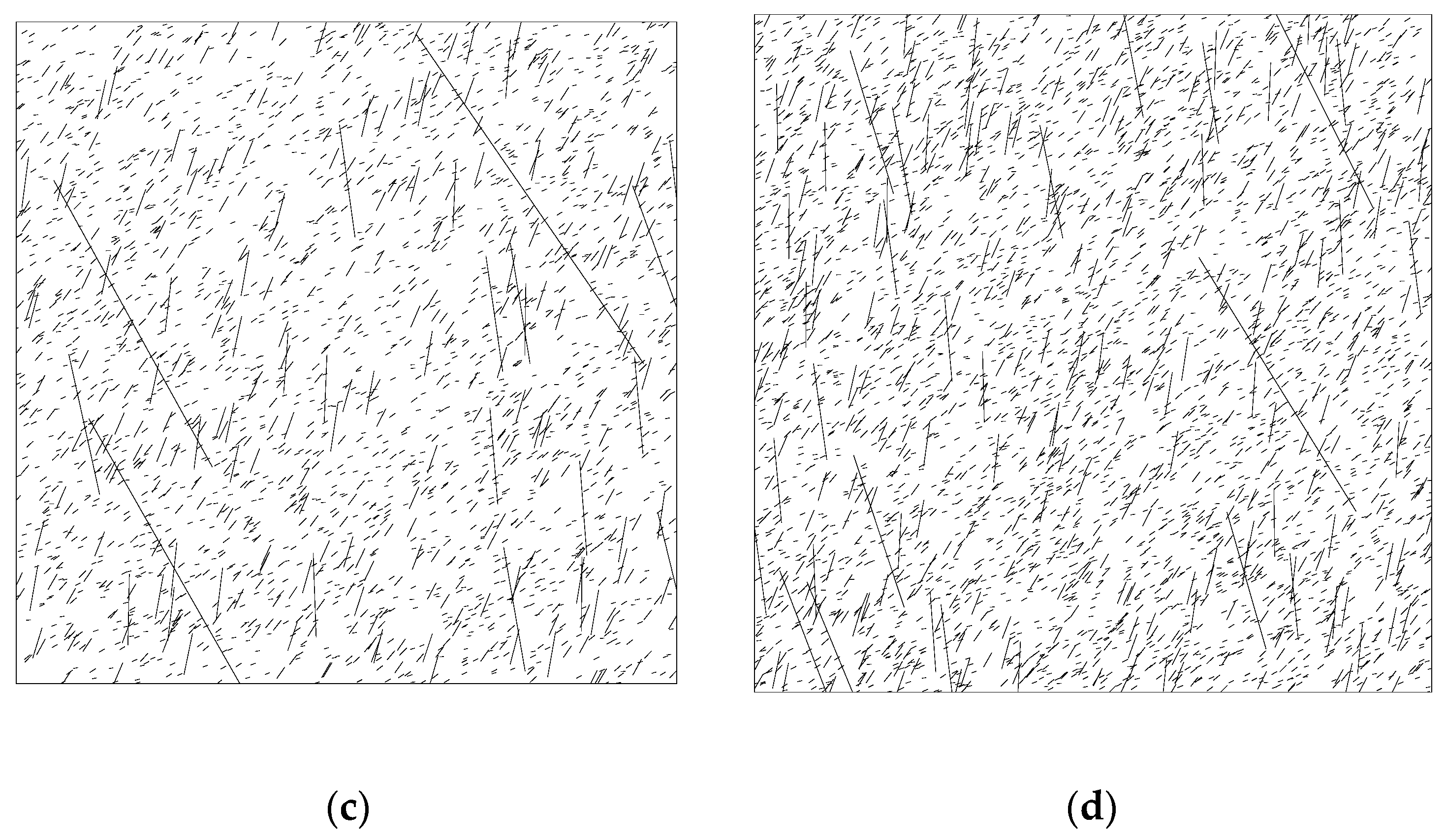
Figure 1 presents four fractal discrete fracture networks. Their fractal dimensions are between 1.5 and 1.8. The parameters used in these models are listed in

Table 1. Parameters used in creation of fractal fracture network model.

Parameter	Value
Fracture network size (m × m)	50 × 50
Fracture length fractal dimension, Dl	1.5–1.8
Maximum fracture length, lmax (m)	30
Minimum fracture length, lmin (m)	0.3
Fisher constant, K	5

. It is clearly seen that the total number of fractures increases rapidly and more fractures with longer fracture length appear when the fractal dimension $D_l$ increases.

2.2. Governing Equations for Multi-Physical Processes in Fractured Shale Reservoirs

The governing equations for the multi-physical processes in fractured shale reservoirs are based on the following assumptions: (a) rock mass is linearly elastic and its strain is infinitesimal [4]; (b) the shale gas is ideal gas; (c) single-phase gas flows in the shale reservoir.

2.2.1. Deformation Equation of the Fractured Shale Reservoir

In our previous studies [11,13], we observed that the effective stress in the shale reservoir and the gas adsorption properties change with the decrease of gas pressure during gas extraction. The variations of effective stress and matrix swelling induced by gas desorption result in shale rock deformation, which alters the permeability in the matrix and fracture and significantly impacts the gas flow in the shale reservoir. The Navier equilibrium equation for the deformation of fractured reservoirs is

$$\mu u_{i,jj}+\left(\lambda +\mu \right)u_{j,ji}-{\alpha }_m{p}_{m,i}-{\alpha }_f{p}_{f,i}-K{\epsilon }_{s,i}+f_i=0,$$

(9)

where $u_i$ is the displacement component; $\mu$ and $\lambda$ are the Lamé constants which are expressed by the Young’s modulus $E$ (MPa) and the Poisson’s ratio $\nu$, $\mu =E/2\left(1+\nu \right)$, $\lambda =E\nu /\left[\left(1+\nu \right)\left(1-2\nu \right)\right]$; $K=E/3\left(1-2\nu \right)$ is the bulk modulus, MPa; ${\alpha }_m$ and ${\alpha }_f$ are the Biot’s coefficient of shale matrix and fractures, respectively; $p_m$ and $p_f$ are the gas pressure in matrix and fractures, respectively, MPa; ${\epsilon }_s={\alpha }_g{V}_a$ is the sorption-induced swelling strain which can be calculated by the multilayer adsorption model [12]; ${\alpha }_g$ is the sorption-induced volumetric strain coefficient, kg/m³; $V_a$ is the adsorbed gas content in matrix, m³/kg; $f_i$ is the body force component.

2.2.2. Equation of Gas Flow in Shale Matrix

The pore size of shale matrix is mainly in nanometer scale [4]. The structure of nanometer pores makes the gas transport mechanisms in shale matrix complex. The slip flow, Knudsen diffusion, molecular diffusion, and surface diffusion may co-exist in shale matrix [4,10,13]. Moreover, a large number of adsorbed gases are stored in the kerogen of shale matrix. It is important to accurately describe these properties of gas adsorption and desorption when the gas production from a shale reservoir is simulated. The most widely used adsorption model in shale reservoirs is the Langmuir isotherm, which is based on the assumption that there is only a monolayer of molecules on the surface of nanopores. However, Yu et al. [9] found that gas adsorption in shale matrix behaves similarly to multilayer adsorption. Their experimental data of adsorption was deviated from the Langmuir isotherm but obeyed the Brunauer–Emmett–Teller (BET) isotherm. The multilayer BET adsorption model can be expressed as

$$V_a=\frac{V_{m}Cx\left[1-\left(n+1\right)x^n+n{x}^{n+1}\right]}{\left(1-x\right)\left[1+\left(C-1\right)x-C{x}^{n+1}\right]},$$

(10)

where $V_m$ is the monolayer saturated adsorption volume, m³/kg; $C$ is a constant; $n$ is the number of adsorption layers; $x=p_m/p_s$ is the relative pressure; $p_s$ is the pseudo-saturation pressure, MPa.

The mass conservation law for the gas flow in shale matrix can be expressed as [4,12]

$$\frac{\partial m_m}{\partial t}-\nabla \left({\rho }_{gm}\frac{k_m}{\eta }\nabla p_m\right)=-Q_{m,f},$$

(11)

where $\eta$ is the gas viscosity in shale matrix, Pa·s; ${\rho }_{gm}$ is the gas density in shale matrix, kg/m³; $Q_{m,f}$ is the mass exchange term between shale matrix and fracture network, kg/(m³·s). The negative sign of $Q_{m,f}$ denotes the gas migration from shale matrix to fracture network.

The mass exchange term $Q_{m,f}$ is expressed as

$$Q_{m,f}=\frac{{\rho }_{gm}{k}_m\delta }{\eta }\left(p_m-p_f\right).$$

(12)

For ideal gas

$${\rho }_{gm}=\frac{M}{RT}{p}_m=\frac{{\rho }_{ga}}{p_a}{p}_m,$$

(13)

where $\delta$ is a geometry factor of shale matrix; $M$ is the average molar mass of methane, kg/mol; $R$ is the universal gas constant, J/(mol·K); $T$ is the reservoir temperature, K; ${\rho }_{ga}$ is the gas density at the standard atmospheric pressure $p_a$ (= 101.325 kPa), kg/m³.

Shale matrix has strong gas storage capacity, in which both adsorbed gas and free gas coexist. Therefore, the gas mass content $m_m$ in shale matrix is

$$m_m={\rho }_{gm}{\varphi }_m+{\rho }_{ga}{\rho }_s\frac{V_{m}Cx\left[1-\left(n+1\right)x^n+n{x}^{n+1}\right]}{\left(1-x\right)\left[1+\left(C-1\right)x-C{x}^{n+1}\right]},$$

(14)

where ${\varphi }_m$ is the porosity of shale matrix; ${\rho }_s$ is the density of shale rock, kg/m³.

$k_m$ is the fractal permeability of shale matrix which can be obtained from the following two steps: Firstly, a permeability model is developed in a single nanopore based on different gas flow mechanisms, such as molecular flow, transition flow, slip flow, and continuum flow [4,12,13]. Then, this permeability model is extended to consider the fractal distribution of pore sizes. The fractal permeability model for the free gas is obtained through the superposition of slip flow and Knudsen diffusion. For adsorbed gas, the molecules transferred in the adsorption multilayer make significant contributions to gas transport in shale matrix, referred to as surface diffusion. Therefore, a fractal permeability of shale matrix $k_m$ is obtained as

$$\begin{array}{lll}{k}_m& =& \underset{k_{m,p}}{\underbrace{\frac{\pi {\varphi }_m{D}_{\lambda }{D}_{\max }^{3+D_{\tau }}}{128L_0^{D_{\tau }+1}\left(3+D_{\tau }-D_{\lambda }\right)}\left[1+\frac{4\eta \left(3+D_{\tau }-D_{\lambda }\right)\left(1-{\zeta }^{2+D_{\tau }-D_{\lambda }}\right)}{D_{\max }\left(2+D_{\tau }-D_{\lambda }\right)p_m}\sqrt{\frac{\pi RT}{2M}}\right]}}\\ & +& \underset{k_{m,k}}{\underbrace{\frac{\eta \pi {\varphi }_m{D}_{\lambda }{D}_{\max }^{4+D_{\tau }-D_{\lambda }}{d}_m^{D_{\lambda }-2}\left(1-{\zeta }^{4+D_{\tau }-2D_{\lambda }}\right)}{12L_0^{D_{\tau }+1}\left(4+D_{\tau }-2D_{\lambda }\right)p_m}\sqrt{\frac{8RT}{\pi M}}}}\\ & +& \underset{k_{m,s}}{\underbrace{\frac{\eta D_s{\rho }_s{p}_a{D}_{\lambda }{D}_{\max }^{D_{\tau }-1}{\varphi }_a\left(1-{\zeta }^{D_{\tau }-D_{\lambda }-1}\right)}{p_m{L}_0^{D_{\tau }-1}\left(D_{\tau }-D_{\lambda }-1\right)}\left[\frac{V_a{p}_s}{p_m\left(p_s-p_m\right)}-a-b\right]}}\end{array}$$

(15)

where $a=\frac{V_{m}C}{p_s}\frac{n\left(n+1\right)x^n}{1+\left(C-1\right)x-C{x}^{n+1}}$ and $b=\frac{V_a}{p_s}\frac{C-1-C\left(n+1\right)x^n}{1+\left(C-1\right)x-C{x}^{n+1}}$; $k_{m,p}$, $k_{m,k}$, and $k_{m,s}$ are the fractal permeability for slip flow, Knudsen diffusion, and surface diffusion of shale matrix, m²; $D_{\lambda }$ is the fractal dimension of pore diameter; $D_{\tau }$ is the tortuosity fractal dimension; $\zeta$ is the ratio of the minimum pore diameter $D_{\min }$ to the maximum pore diameter; $D_{\max }$ is the maximum pore diameter, nm; $d_m$ is the methane molecular diameter, nm; $D_s$ is the coefficient of surface diffusion in matrix pores, m²/s; ${\varphi }_a$ is the porosity of adsorbed gas; $L_0$ is the straight length of representative elementary volume (REV) in shale matrix.

By substituting Equations (12)–(15) into Equation (11), the governing equation of gas flow in shale matrix becomes

$$\left[{\varphi }_m+p_a{\rho }_s\left(\frac{V_a}{p_m\left(1-x\right)}-a-b\right)\right]\frac{\partial p_m}{\partial t}-\nabla \left(\frac{p_m{k}_m}{\eta }\nabla p_m\right)=-\frac{\delta p_m{k}_m}{\eta }\left(p_m-p_f\right).$$

(16)

2.2.3. Gas Flow Equation in Fracture Network

Only free gas exists in fractures. The continuity equation for gas flow in the fracture network is expressed as

$$d_f\frac{\partial {\rho }_{gf}{\varphi }_f}{\partial t}+{\nabla }_T\left(-d_f{\rho }_{gf}\frac{k_f}{\eta }{\nabla }_T{p}_f\right)=d_f{Q}_{m,f},$$

(17)

where ${\varphi }_f$ is the porosity of the fracture network; $k_f$ is the permeability of the fracture network, m²; $d_f$ is the aperture of fracture, mm; ${\rho }_{gf}$ is the gas density in the fracture which is expressed as

$${\rho }_{gf}=\frac{{\rho }_{ga}}{p_a}{p}_f.$$

(18)

The permeability of the fracture network is sensitive to the gas pressure and effective stress in the process of gas extraction. The decline of gas pressure results in the increase of effective stress and rock deformation of shale reservoirs, thus altering the permeability of the fracture network with the following formula:

$$k_f=k_{f0}\left\{-3c_f\left[\left(\sigma -{\sigma }_0\right)-\left(p_f-p_{f0}\right)\right]\right\},$$

(19)

where $\sigma$ is the mean normal stress, MPa; ${\sigma }_0$ is the initial mean normal stress, MPa; $p_{f0}$ is the initial gas pressure in the fracture network, MPa; $c_f$ is the compressibility coefficient of the fracture network, 1/MPa; $k_{f0}$ is the initial permeability of fracture network, m².

The decrease of gas pressure and the increase of effective stress can lead to the deformation of shale rock. In the meantime, the rock deformation changes the fracture aperture and further enhances the fracture permeability. The fracture aperture $d_f$ under normal stress can have contributions from both “hard” and “soft” parts [4,36,37]. The relationship between fracture aperture and normal stress is

$$d_f=d_r+d_t\exp \left(-c_f{\sigma }_n\right),$$

(20)

where $d_r$ is the fracture aperture of the “hard” part that does not change with stress, mm; $d_t$ is the true aperture of the “soft” part, mm.

The porosity of the fracture network depends on fracture aperture, which is defined as

$$\frac{{\varphi }_f}{{\varphi }_{f0}}=\frac{d_f}{d_0}=\frac{d_r+d_t\exp \left(-c_f{\sigma }_n\right)}{d_0},$$

(21)

where $d_0$ is the initial fracture aperture, mm.

2.2.4. Gas Flow Equation in Hydraulic Fractures

The gas flow equation in hydraulic fractures is expressed as [13]

$$d_{hf}\frac{\partial \left({\rho }_{ghf}{\varphi }_{hf}\right)}{\partial t}+\nabla \left(-\frac{k_{hf}}{\eta }{d}_{hf}{\rho }_{ghf}\nabla p_{hf}\right)=0,$$

(22)

where ${\varphi }_{hf}$, $k_{hf}$, ${\rho }_{ghf}$, $d_{hf}$, and $p_{hf}$ are the porosity, permeability (m²), gas density (kg/m³), aperture (mm), and gas pressure (MPa) of hydraulic fractures, respectively.

3. Implementation and Validation of Proposed Numerical Model

3.1. Geometry of Numerical Simulation Model

A multi-staged fracturing horizontal well is schematically illustrated in Figure 2a. The red horizontal line denotes the horizontal well, and the blue vertical lines represent hydraulic fractures. The black lines with different lengths are fractures to form a fracture network in the shale gas reservoir. The numerical simulation is difficult due to the large size of the whole shale reservoir and the numerous fractures. In order to reduce numerical simulation loading, half of the domain between two adjacent hydraulic fractures is chosen as the simulation domain. Its 2D simulation model with dimensions of 50 m × 50 m is shown in Figure 2b. The fracture network is created through the previously-mentioned fractal distribution of fracture lengths. The simulation model in Figure 2b is the same as Figure 1a where the fractal dimension of the fracture length is 1.5. The right and left boundaries are the hydraulic fractures and the bottom boundary is the horizontal well.

3.2. Multi-Physical Coupling During Gas Extraction

The deformation equation (Equation (9)) and the gas flow equations in shale matrix (Equation (16)), the fracture network (Equation (17)), and hydraulic fractures (Equation (22)) are fully coupled during gas extraction. In the deformation process, the normal stress on the top boundary is 40 MPa and the other three boundaries are roller boundary conditions (see Figure 2b), which are used to simulate the in-situ stress state. For the gas flow in shale matrix, the four boundaries are all no flux. Fractures are the flow boundaries in matrix. The gas pressure is continuous at the interface between fractures and matrix. The gas flow equations of the fracture network and hydraulic fractures are solved by the fracture flow module. The unstructured grid is used to mesh the model due to numerous fractures. After meshing, the whole computing domain contains 18,238 elements. The solution time of the common computer with i7-9750H CPU and 8GB RAM is 8 min and 11 s.

3.3. Model Reliability

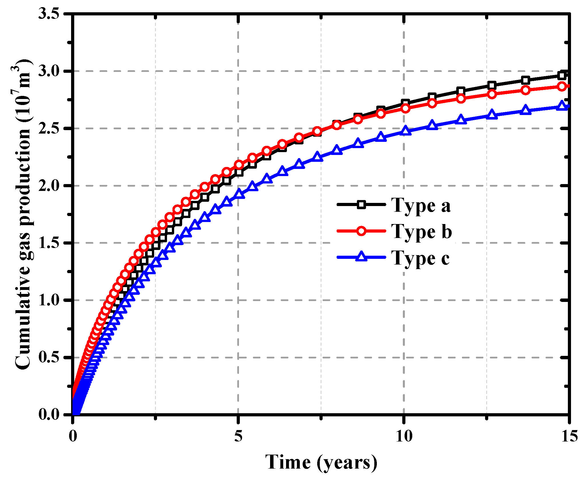
As the position and orientation of the fractal discrete fracture network are random, the reliability of the numerical model should be checked first. When the fractal discrete fracture network is created, the position and orientation of fractures are only changed at fixed other parameters. Figure 3 shows three different types of fractal discrete fracture networks. The fractures have different positions and directions, but the same length distribution and the total number of fractures because they are created with the same parameters. All the parameters used in numerical simulations are listed in

Table 2. All parameters used in numerical simulations.

Parameters	Values
Initial reservoir gas pressure, $p_0$ (MPa)	25
Bottom pressure, (MPa)	3.0
Reservoir temperature, $T$ (K)	330
Thickness of fracture network model, $H$ (m)	10
Universal gas constant, $R$ (J/(mol·K))	8.314
Molar mass of methane, $M$ (kg/mol)	0.016
Molecular diameter of methane, $d_m$ (nm)	0.38
Straight length of representative elementary volume (REV) in matrix, $L_0$ (mm)	0.1
Density of shale reservoir, ${\rho }_s$ (kg/m3)	2580
Young’s modulus of shale, $E$ (GPa)	20
Poisson’s ratio of shale, $\nu$	0.3
Methane dynamic viscosity, $\eta$ (Pa·s)	1.2 × 10−5
Gas density at standard condition, ${\rho }_{ga}$ (kg/m3)	0.717
Porosity of hydraulic fractures, ${\varphi }_{hf}$	0.001
Permeability of hydraulic fractures, $k_{hf}$ (m2)	5 × 10−10
Aperture of hydraulic fractures, $d_{hf}$ (mm)	0.3
Geometry factor, $\delta$	1
Initial porosity of fractures, ${\varphi }_{f0}$	0.005
Initial permeability of fractures, $k_{f0}$ (m2)	5 × 10−13
Proportionality coefficient, $\gamma$	0.001
Compressibility of the fractures, $c_f$ (1/MPa)	5.0 × 10−4
Fracture aperture of the “hard” part, $d_r$ (mm)	0.1
Fracture aperture of the “soft” part, $d_t$ (mm)	0.1
Initial fracture aperture, $d_0$ (mm)	0.1
Adsorption volume in monolayer, $V_m$ (cm3/g)	1.63
Pseudo-saturation pressure, $p_s$ (MPa)	100
Number of adsorption layer, $n$	5.54
Constant, $C$	26.39
Porosity of adsorbed gas, ${\varphi }_a$	0.05
Porosity of shale matrix, ${\varphi }_m$	0.15
Diameter fractal dimension, $D_{\lambda }$	2.7
Tortuosity fractal dimension, $D_{\tau }$	1.1
Maximum pore diameter, $D_{\max }$ (nm)	1000
Minimum pore diameter, $D_{\min }$ (nm)	10
Sorption-induced strain coefficient, ${\alpha }_g$ (kg/m3)	0.75
Surface diffusion coefficient, $D_s$ (m2/s)	1 × 10−10
Biot’s coefficient of matrix, ${\alpha }_m$	0.5
Biot’s coefficient of fractures, ${\alpha }_f$	0.5

. In the fracture network, the fractures are the main gas flow channels for gas production. The gas flow rate of this fracture network model can be calculated by the line integral of discrete fractures under the standard condition (293.15 K, 101.325 kPa):

$$Q=24\times 3600\times \frac{H}{{\rho }_{ga}}\int {\nu }_{f}ds=24\times 3600\times \frac{H}{{\rho }_{ga}}\int {\rho }_{gf}\frac{k_f}{\eta }\nabla p_{f}ds,$$

(23)

where $Q$ is the gas flow rate, m³/d; $H$ is the thickness of the fracture network model, m. The cumulative gas production can be expressed as

$$V_t={\int }_0^{t}Qdt,$$

(24)

where $V_t$ is the cumulative gas production, m³.

The cumulative gas production from three types of fractal discrete fracture networks is presented in Figure 4. At the 15th year, the cumulative gas production for type a, b, and c is 2.96 × 10⁷ m³, 2.86 × 10⁷ m³, and 2.69 × 10⁷ m³, respectively. Their average is 2.84 × 10⁷ m³. These results show that their cumulative gas production slightly varies with fracture pattern. The difference of cumulative gas production is 3.4% between type a and b, 5.9% between type b and c, and 9.1% between type c and a. The biggest difference compared to their average is 5.3%. This difference is acceptable for a random medium. This means that the random process of the position and orientation of the fracture network can induce some, but ignorable, differences. The numerical simulation results with any fractal discrete fracture network are reliable and acceptable.

3.4. Model Accuracy Check

The gas production data from two shale wells in the Marcellus shale and the Barnett shale are used to verify the simulation model. The reservoir parameters of these two shale wells are determined based on literature [10,11,12,38] and listed in

Table 3. Reservoir parameters for the Marcellus shale and Barnett shale wells.

Parameters	Marcellus Shale	Barnett Shale	Unit
Initial reservoir gas pressure	34.5	20.34	MPa
Bottom pressure	2.4	3.69	MPa
Porosity of hydraulic fractures	1 × 10−6	1 × 10−6
Permeability of hydraulic fractures	3 × 10−10	5 × 10−9	m2
Initial porosity of fractures	0.005	0.002
Initial permeability of fractures	1 × 10−20	1.9×10−13
Adsorption volume in monolayer	1.63	1.18	cm3/g
Porosity of shale matrix	0.15	0.15
Fracture length fractal dimension	1.5	1.7
Diameter fractal dimension	2.85	2.64
Tortuosity fractal dimension	1.1	1.2
Maximum pore diameter	600	1000	nm
Minimum pore diameter	10	10	nm

. The comparison between field data and numerical simulations is shown in Figure 5 for the Marcellus shale well (90 data points over 280 days) and in Figure 6 for the Barnett shale well (134 data points over 1630 days). For the Marcellus shale well in Figure 5, a small difference is observed in the initial stage of gas production where the simulation results are smaller than the field data. Liu et al. [22] also observed a similar phenomenon. However, the simulation results for the Barnett shale well are much lower than the field data in the initial stage of gas production (see Figure 6). This may be due to the effects of local heterogeneity of fracture deformation. The aperture of the “soft” part can easily change with normal stress. The local heterogeneity of deformation is from the compression of the “soft” part and reduces the aperture of the fracture. The gas flow resistance in fractures is large due to the small aperture, which results in lower gas production rates [4]. With the increase of extraction time, the effect of deformation on gas production rate becomes weak. Thus, the differences between the field data and simulation results become small in the later stage. Our simulation results match well with the field gas production data from the two shale wells. This implies that our simulation model is feasible in describing the shale gas production with sufficient accuracy.

4. Results and Discussions

4.1. Effects of Fracture Length Fractal Dimension

Fracture length fractal dimension is a key parameter to a fracture network. This section will investigate the effects of fracture length fractal dimension on the variation of reservoir pressure and shale gas production.

4.1.1. Variation of Reservoir Pressure

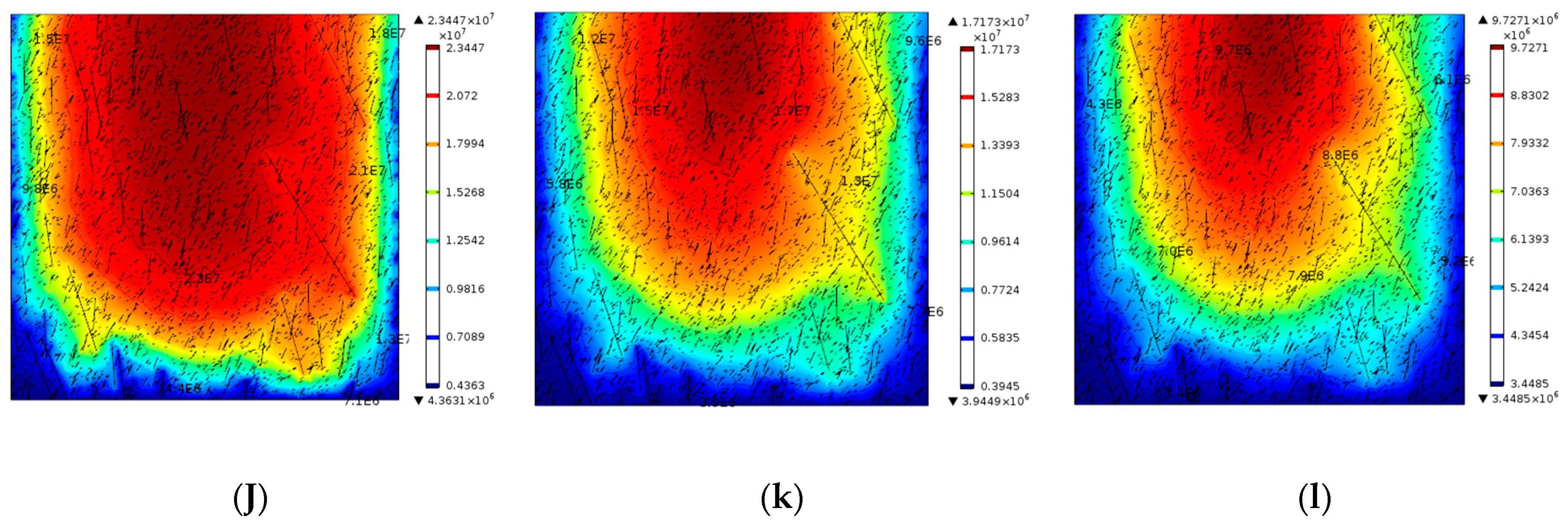
The variation of reservoir pressure with time is studied. Figure 7 shows the reservoir pressure distributions in the reservoir when these four fracture networks are used, respectively. The reservoir pressure firstly dissipates near the horizontal well and the hydraulic fractures due to their high permeability. With the extraction time, the pressure decreases, and the drainage area increases significantly, especially around the discrete fractures. A bigger drainage area means more gas depleted from the shale gas reservoir. Thus, the gas flow process in the shale gas reservoir is dynamic. Shale gas is first depleted from the hydraulic fractures, then from the fracture network. Finally, the gas in shale matrix enters the fracture network through desorption and diffusion. The fracture network becomes much more complex when the fracture length fractal dimension increases from 1.5 to 1.8. The fracture network whose length fractal dimension is 1.8 has the largest total number of fractures, the largest drainage area, and the fastest reservoir pressure drop. That is, the complex fracture network can extend the decline of reservoir pressure to a larger drainage area.

4.1.2. Impacts of Fracture Network on Shale Gas Production

The effects of fractal dimension on gas production rate are presented in Figure 8. The gas production rate is the lowest at $D_l=1.5$ and the largest at $D_l=1.8$. The production decline at $D_l=1.8$ is the fastest in the initial stage; this is because the fracture network of $D_l=1.8$ is the most complex and the total number of fractures is 3982 (see Figure 1), which is larger than those with other fractal dimensions. The amplitude of free gas in fractures supports the gas production rate in the initial stage. With the increase of extraction time, the free gases in the fracture network of $D_l=1.8$ are soon exhausted and the gas production rate is lower than that of $D_l=1.7$. The effects of fractal dimension on cumulative gas production are shown in Figure 9. The cumulative gas production after 15 years increases from 4.6 × 10⁷ m³ to 9.8 × 10⁷ m³. When the fractal dimension increases from 1.5 to 1.7, the increase rate is 113%. This is because a larger fractal dimension means much more flow channels to hydraulic fractures and the horizontal well. However, there is a phenomenon worthy of attention. The cumulative gas production of $D_l=1.8$ is 9.1 × 10⁷ m³, which is lower than that of $D_l=1.7$ after 15 years. The reason is that the highest gas production rate of $D_l=1.8$ in the initial stage leads to a rapid drop in gas pressure and a fast decline of reservoir storage, which reduces the production capacity of the reservoir. Before the fractal dimension reaches a certain value, the cumulative gas production increases with the increase of fractal dimension. The critical fractal dimension is 1.7 in this paper. When the fractal dimension reaches its critical value, the increase of the fractal dimension no longer enhances gas production. It may reduce the production capacity of the shale reservoir. Thus, properly increasing the number and fractal dimension of fractures in a certain range can effectively enhance the shale gas recovery.

4.2. Effects of Pore Size Distribution

A large quantity of gas stores in shale matrix pores and plays an important role in gas production. Thus, the effects of pore size distribution on gas production should be investigated. Figure 10 shows the effects of maximum pore diameter $D_{\max }$ and minimum pore diameter $D_{\min }$ on the cumulative gas production. In Figure 10a, the minimum pore diameter $D_{\min }$ is fixed to 10 nm and the maximum pore diameter $D_{\max }$ is taken as 500 nm, 700 nm, 900 nm, and 1100 nm, respectively. These figures show that the cumulative gas production increases with the increase of maximum pore diameter. It may be because the larger the pore diameter, the more gas storage space, and the easier the gas flow. For the curves of $D_{\max }=900\mathrm{nm}$ and $D_{\max }=1100\mathrm{nm}$, the biggest difference of cumulative gas production between the two curves is 27.9% at about four years, but the two curves are almost identical at 12 years. The reason is that faster gas flow rate in the early stage leads to faster gas exhaustion of shale gas reservoir, which slows down the increase of cumulative gas production in the late stage. The effects of minimum pore diameter on cumulative gas production are shown in Figure 10b. This cumulative gas production increases with the decrease of minimum pore diameter. This is opposite to the effect of the maximum pore diameter. This is because smaller minimum pore diameter results in a larger range of pore size. Thus, the total number of pores is much larger when the minimum pore diameter is smaller, which further enhances the permeability of shale matrix.

4.3. Effects of Initial Fracture Permeability

The fracture network is the main gas flow channel and plays an important role in gas extraction from a shale gas reservoir. The fracture permeability is the key parameter affecting gas flow resistance. It is necessary to investigate the effects of fracture permeability on gas production.

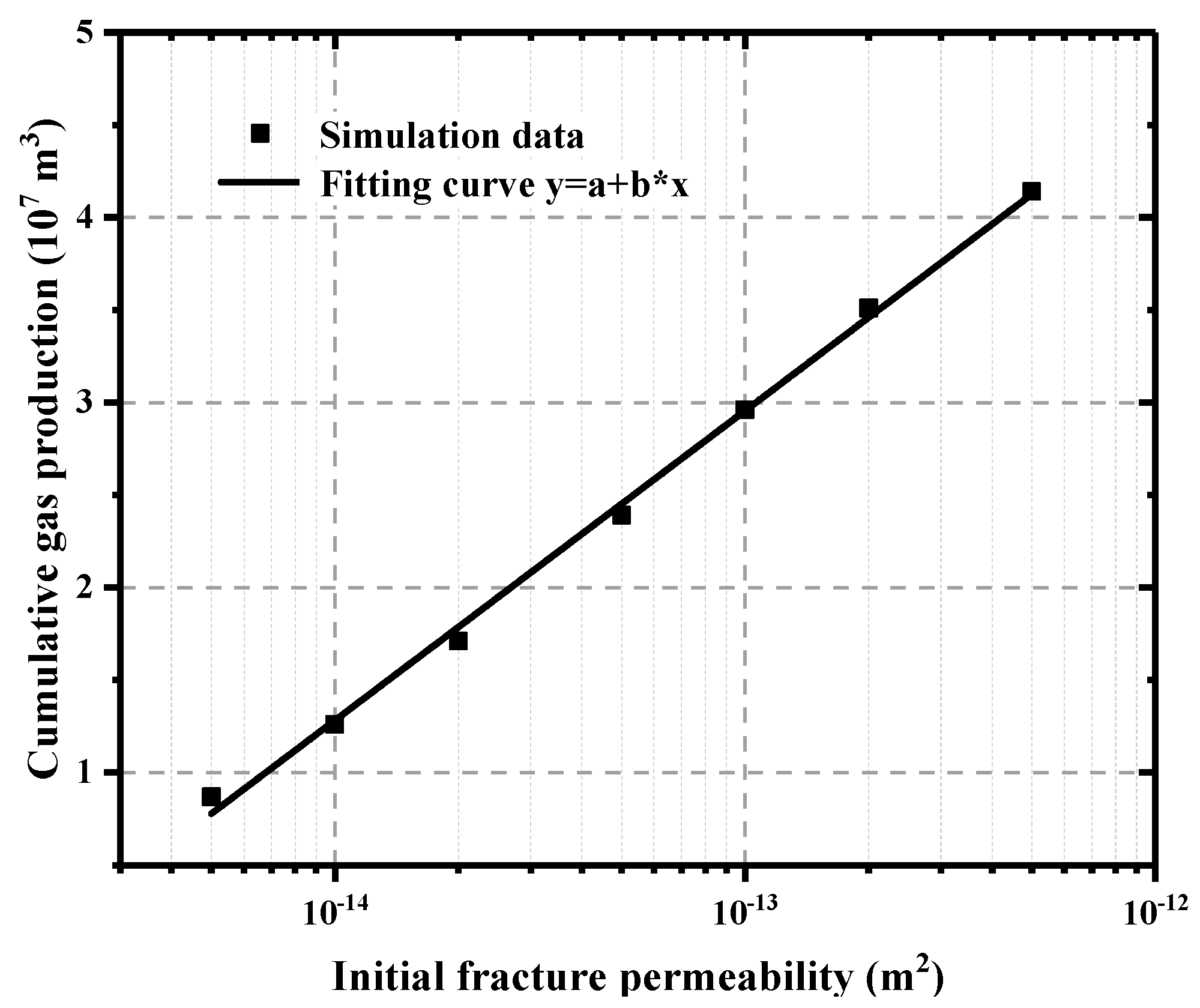
The effects of initial fracture permeability on cumulative gas production are presented in Figure 11. The cumulative gas production increases with the increase of initial fracture permeability and a great influence on gas production is observed. When the initial fracture permeability increases from 5 × 10⁻¹⁵ m² to 5 × 10⁻¹⁴ m² and 5 × 10⁻¹³ m², the cumulative gas production increases from 8.9 × 10⁶ m³ to 2.4 × 10⁷ m³ and 4.1 × 10⁷ m³ after 3000 days, respectively. The relationship between cumulative gas production and initial fracture permeability is shown in Figure 12. A good linear relationship with an R² of 0.99 is observed. Thus, the contribution of initial fracture permeability to the cumulative gas production increases approximately linearly with the increases of fracture permeability. Enhancing the initial fracture permeability is a very useful method to enhance gas production.

5. Conclusions

A new fractal discrete fracture network model was created based on the fractal length distribution and incorporated into a numerical simulation model to evaluate the gas well performance of a fractured shale gas reservoir. This numerical simulation model of a fractured shale gas reservoir fully coupled the fractal discrete fracture network model, the fractal properties of pore size, and multiple gas flow mechanisms, such as slip flow, Knudsen diffusion, surface diffusion, and multilayer adsorption. The reliability and accuracy of the numerical simulation model were validated by the field gas production data from two shale wells. The sensitivity analyses were conducted on the impacts of fractal dimension, pore size distribution, and fracture permeability on gas production. From these studies, the following conclusions can be drawn:

Firstly, the new simulation model for the fractal discrete fracture network is proposed to evaluate the gas production for a fractured shale reservoir. This simulation model can describe the gas well performance of the fractured shale reservoir and is reliable and accurate in the prediction of shale production.

Secondly, the fractal length distribution has different effects of gas production at different stages of gas production. In the early stage, the gas production rate and cumulation gas production increase with the increase of fractal length dimension. After this parameter increases to a critical value of 1.7, the production capacity of the shale reservoir decreases rapidly. This induces the rapid gas production rate in the early stage and leads to fast depletion of reservoir storage in the later stage.

Thirdly, increasing the maximum pore diameter and decreasing the minimum pore diameter can increase the matrix permeability, which will enhance the reservoir gas recovery. The effect of pore size distribution on cumulative gas production is up to 27.9%, which cannot be ignored in the prediction of shale gas production.

Lastly, the cumulative gas production increases with an increase of fracture permeability. An obvious linear relationship can be observed between the cumulative gas production and fracture permeability.

References

- Chapman, M.; Palisch, T. Fracture conductivity-Design considerations and benefits in unconventional reservoirs. J. Pet. Sci. Eng. 2014, 124, 407–415. [Google Scholar] [CrossRef]
- Patzek, T.; Male, F.; Marder, M. A simple model of gas production from hydrofractured horizontal wells in shales. AAPG Bull. 2014, 98, 2507–2529. [Google Scholar] [CrossRef]
- AlTwaijri, M.; Xia, Z.; Yu, W.; Qu, L.; Hu, Y.; Xu, Y.; Sepehrnoori, K. Numerical study of complex fracture geometry effect on two-phase performance of shale-gas wells using the fast EDFM method. J. Pet. Sci. Eng. 2018, 164, 603–622. [Google Scholar] [CrossRef]
- Wang, J.G.; Hu, B.; Liu, H.; Han, Y. Effects of ‘soft-hard’ compaction and multiscale flow on the shale gas production from a multistage hydraulic fractured horizontal well. J. Petrol. Sci. Eng. 2018, 170, 873–887. [Google Scholar] [CrossRef]
- Zhang, L.; Cui, C.; Ma, X.; Sun, Z.; Liu, F.; Zhang, K. A fractal discrete fracture network model for history matching of naturally fractured reservoirs. Fractals 2019, 27, 1–15. [Google Scholar] [CrossRef]
- Civan, F. Effective correlation of apparent gas permeability in tight porous media. Transp. Porous Media 2010, 82, 375–384. [Google Scholar] [CrossRef]
- Akkutlu, I.Y.; Fathi, E. Multiscale gas transport in shales with local kerogen heterogeneities. SPE J. 2012, 17, 1002–1011. [Google Scholar] [CrossRef] [Green Version]
- Darabi, H.; Ettehad, A.; Javadpour, F.; Sepehrnoori, K. Gas flow in ultra-tight shale strata. J. Fluid Mech. 2012, 710, 641–658. [Google Scholar] [CrossRef]
- Yu, W.; Sepehrnoori, K.; Patzek, T. Modeling gas adsorption in Marcellus shale with Langmuir and BET isotherms. SPE J. 2016, 21, 589–600. [Google Scholar] [CrossRef] [Green Version]
- Geng, L.; Li, G.; Wang, M.; Li, Y.; Tian, S.; Pang, W.; Lyu, Z. A fractal production prediction model for shale gas reservoirs. J. Nat. Gas Sci. Eng. 2018, 55, 354–367. [Google Scholar] [CrossRef]
- Hu, B.; Wang, J.G.; Li, Z.; Wang, H. Evolution of fractal dimensions and gas transport models during the gas recovery process from a fractured shale reservoir. Fractals 2019, 27, 1950129. [Google Scholar] [CrossRef]
- Hu, B.; Wang, J.G.; Wu, D.; Wang, H. Impacts of zone fractal properties on shale gas productivity of a multiple fractured horizontal well. Fractals 2019, 27, 1950006. [Google Scholar] [CrossRef]
- Wang, J.G.; Hu, B.; Wu, D.; Dou, F.; Wang, X. A multiscale fractal transport model with multilayer sorption and effective porosity effects. Transp. Porous Media 2019, 129, 25–51. [Google Scholar] [CrossRef]
- Wang, H.; Wang, J.G.; Wang, X.; Hu, B. An improved relative permeability model for gas-water displacement in fractal porous media. Water 2020, 12, 27. [Google Scholar] [CrossRef] [Green Version]
- Klimczak, C.; Schultz, R.A.; Parashar, R.; Reeves, D.M. Cubic law with aperture-length correlation: Implications for network scale fluid flow. Hydrogeol. J. 2010, 18, 851–862. [Google Scholar] [CrossRef]
- Larsen, B.; Grunnaleite, I.; Gudmundsson, A. How fracture systems affect permeability development in shallow-water carbonate rocks: An example from the Gargano Peninsula, Italy. J. Struct. Geol. 2010, 32, 1212–1230. [Google Scholar] [CrossRef]
- Ambrose, R.J.; Hartman, R.C.; Diaz-Campos, M.; Akkutlu, I.Y.; Sondergeld, C.H. Shale gas-in-place calculations part I: New pore-scale considerations. SPE J. 2012, 17, 219–229. [Google Scholar] [CrossRef]
- Jafari, A.; Babadagli, T. Estimation of equivalent fracture network permeability using fractal and statistical network properties. J. Pet. Sci. Eng. 2012, 92–93, 110–123. [Google Scholar] [CrossRef]
- Miao, T.; Yu, B.; Duan, Y.; Feng, Q. A fractal analysis of permeability for fractured rocks. Int. J. Heat Mass Transf. 2015, 81, 75–80. [Google Scholar] [CrossRef]
- Warren, J.E.; Root, P.J. The behavior of naturally fractured reservoirs. Soc. Petrol. Eng. J. 1963, 3, 245–255. [Google Scholar] [CrossRef] [Green Version]
- Liu, J.; Wang, J.G.; Leung, C.F.; Gao, F. A multi-parameter optimization model for the evaluation of shale gas recovery enhancement. Energies 2018, 11, 654. [Google Scholar] [CrossRef] [Green Version]
- Liu, J.; Wang, J.G.; Gao, F.; Ju, Y.; Zhang, X.; Zhang, L. Flow consistency between non-Darcy flow in fracture network and nonlinear diffusion in matrix to gas production rate in fractured shale gas reservoirs. Transp. Porous Media 2016, 111, 97–121. [Google Scholar] [CrossRef]
- Liu, J.; Wang, J.G.; Gao, F.; Leung, C.F.; Ma, Z. A fully coupled fracture equivalent continuum-dual porosity model for hydro-mechanical process in fractured shale gas reservoirs. Comput. Geotech. 2019, 106, 143–160. [Google Scholar] [CrossRef]
- Jiang, J.; Younis, R. A multimechanistic multicontinuum model for simulating shale gas reservoir with complex fractured system. Fuel 2015, 161, 333–344. [Google Scholar] [CrossRef]
- Yu, W.; Xu, Y.; Liu, M.; Wu, K.; Sepehrnoori, K. Simulation of shale gas transport and production with complex fractures using embedded discrete fracture model. AIChE J. 2018, 64, 2251–2264. [Google Scholar] [CrossRef]
- Cao, R.; Fang, S.; Jia, P.; Cheng, L.; Rao, X. An efficient embedded discrete-fracture model for 2D anisotropic reservoir simulation. J. Pet. Sci. Eng. 2019, 174, 115–130. [Google Scholar] [CrossRef]
- Akkutlu, I.Y.; Efendiev, Y.; Vasilyeva, M. Multiscale model reduction for shale gas transport in fractured media. Comput. Geosci. 2016, 20, 953–973. [Google Scholar] [CrossRef] [Green Version]
- Akkutlu, I.Y.; Efendiev, Y.; Vasilyeva, M.; Wang, Y. Multiscale model reduction for shale gas transport in a coupled discrete fracture and dual-continuum porous media. J. Nat. Gas Sci. Eng. 2017, 48, 65–76. [Google Scholar] [CrossRef]
- Odling, N.E. Scaling and connectivity of joint systems in sandstones from western Norway. J. Struct. Geol. 1997, 19, 1251–1271. [Google Scholar] [CrossRef]
- Baghbanan, A.; Jing, L. Hydraulic properties of fractured rock masses with correlated fracture length and aperture. Int. J. Rock Mech. Min. Sci. 2007, 44, 704–719. [Google Scholar] [CrossRef]
- Parashar, R.; Reeves, D. On iterative techniques for computing flow in large two-dimensional discrete fracture networks. J. Comput. Appl. Math. 2012, 236, 4712–4724. [Google Scholar] [CrossRef] [Green Version]
- Miao, T.; Chen, A.; Xu, Y.; Cheng, S.; Yu, B. A fractal permeability model for porous–fracture media with the transfer of fluids from porous matrix to fracture. Fractals 2019, 26, 1–9. [Google Scholar] [CrossRef]
- Liu, R.; Li, B.; Jiang, Y. A fractal model based on a new governing equation of fluid flow in fractures for characterizing hydraulic properties of rock fracture networks. Comput. Geotech. 2016, 75, 57–68. [Google Scholar] [CrossRef]
- Liu, R.; Yu, L.; Jiang, Y. Fractal analysis of directional permeability of gas shale fracture networks: A numerical study. J. Nat. Gas Sci. Eng. 2016, 33, 1330–1341. [Google Scholar] [CrossRef] [Green Version]
- Priest, S. Discontinuity Analysis for Rock Engineering; Springer: Dordrecht, The Netherlands, 1993. [Google Scholar]
- Liu, H.; Rutqvist, J.; Berryman, J. On the relationship between stress and elastic strain for porous and fractured rock. Int. J. Rock Mech. Min. Sci. 2009, 46, 289–296. [Google Scholar] [CrossRef] [Green Version]
- Shang, X.; Wang, J.G.; Zhang, Z.; Gao, F. A three-parameter permeability model for cracking process of fractured rocks under temperature change and external loading. Int. J. Rock Mech. Min. Sci. 2019, 123, 104106. [Google Scholar] [CrossRef]
- Yu, W.; Sepehrnoori, K. Simulation of gas desorption and geomechanics effects for unconventional gas reservoirs. Fuel 2014, 116, 455–464. [Google Scholar] [CrossRef]
Figure 1.
Four fractal discrete fracture networks with different fractal dimensions: (a) fractal length dimension , and total fracture number ; (b) fractal length dimension , and total fracture number ; (c) fractal length dimension , and total fracture number ; (d) fractal length dimension , and total fracture number .
Figure 2.
Schematic of (a) fractured shale reservoir model; (b) simulation fracture network model geometry.
Figure 3.
Three types of fractal discrete fracture networks: (a) type a; (b) type b; (c) type c.
Figure 4.
Cumulative gas production from a fractured reservoir with three fractal discrete fracture networks.
Figure 5.
Comparison between our simulation results and the field data from the Marcellus shale well.
Figure 6.
Comparison between our simulation results and the field data from the Barnett shale well.
Figure 7.
Reservoir pressure variation with time at different fractal dimensions of fracture length: (a) one month and ; (b) one year and ; (c) three years and ; (d) one month and ; (e) one year and ; (f) three years and ; (g) one month and ; (h) one year and ; (i) three years and ; (j) one month and ; (k) one year and ; (l) three years and .
Figure 8.
Gas production rate from the fracture network with different length fractal dimensions.
Figure 9.
Cumulative gas production from the fracture network with different length fractal dimensions.
Figure 10.
Effects of extreme pore diameters on cumulative gas production: (a) maximum pore diameter ; (b) minimum pore diameter .
Figure 11.
Effects of initial fracture permeability on cumulative gas production.
Figure 12.
Linear relationship between cumulative gas production and initial fracture permeability.