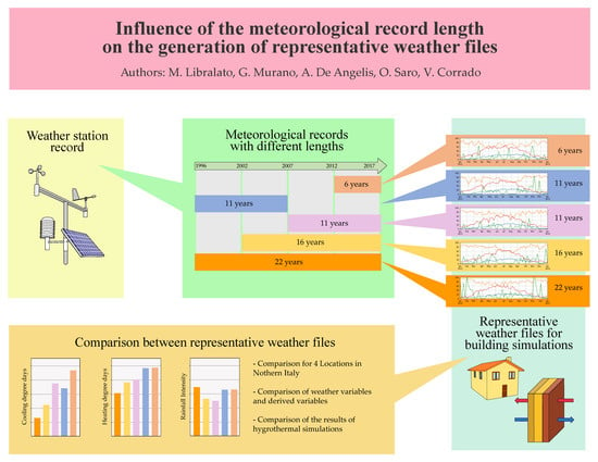
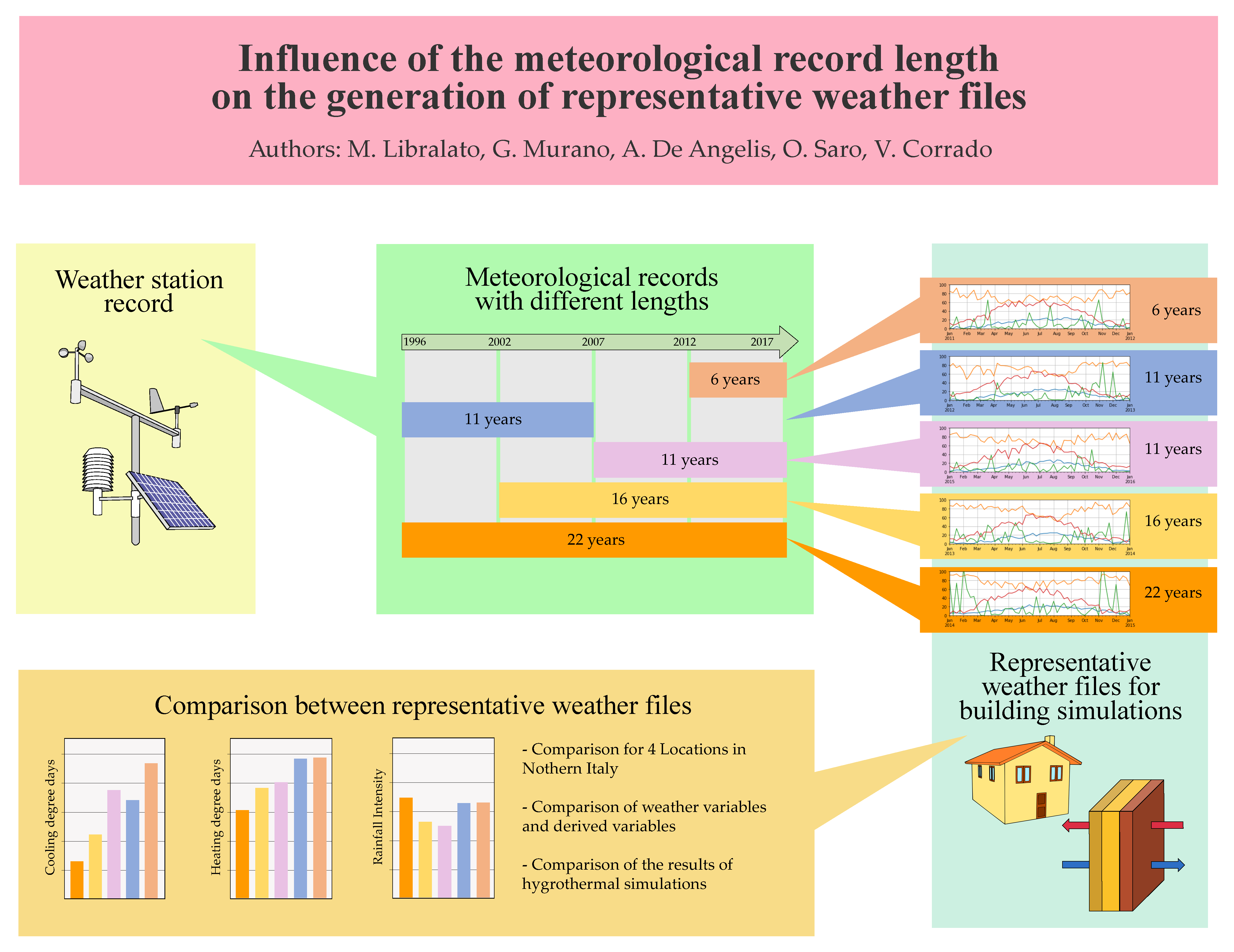
Influence of the Meteorological Record Length on the Generation of Representative Weather Files †

 , , , and
Abstract
:
1. Introduction
1.1. Heat and Moisture Transfer Simulations
1.2. Moisture Representative Year
1.3. Meteorological Record Length
2. Theory
2.1. Methodology for the Construction of the MRY
- (a)
- Calculation the daily means of the primary variables p for the whole MY.
- (b)
- Calculation of the cumulative distribution function of the daily means over the whole MY for each day i of a selected calendar month m, for each p. The variable i represents the ordered number of a day in the MY, from 1 to N (number of days in the MY), and it will be used as a time-stamp. The function is obtained from the ranking by numbering the values of the distributions of the considered p, separately for each m:
- (c)
- Calculation of the cumulative distribution function of the daily means within each calendar month m of each year y, from the rank order , obtained ordering the daily means within the calendar month m and the year y:where n is the number of days of the m calendar month considered.
- (d)
- The Finkelstein–Schafer statistic is calculated for each p and each calendar month m in the MY as:
- (e)
- For each p, the ranking R is assigned to each calendar month m, obtained from the ordering of the of each y separately for each calendar month m:with the number of years of the MY.
- (e)
- The ranking R of each calendar month is calculated for all the primary parameters and then summed, to obtain the total ranking :
- (e)
- Each calendar month m of the MRY is chosen among the months of the MY as the month m of the year y with the lowest .
- (e)
- The MRY is composed by the hourly series of the weather variables of the selected months and the continuity between every month is set with a linear interpolation, in order to provide a smooth transition between months from different years.
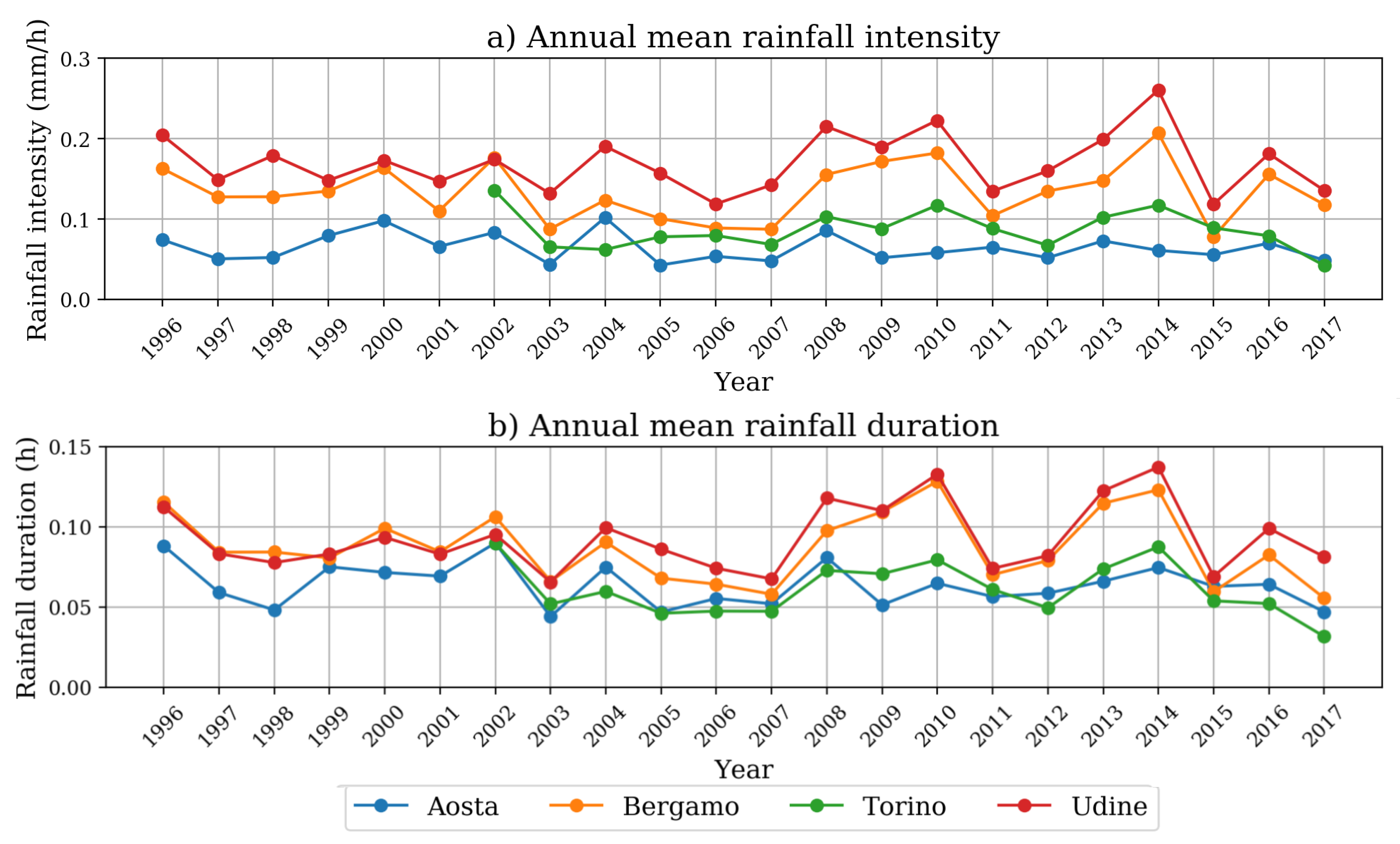
2.2. Rainfall Duration
3. Materials and Methods
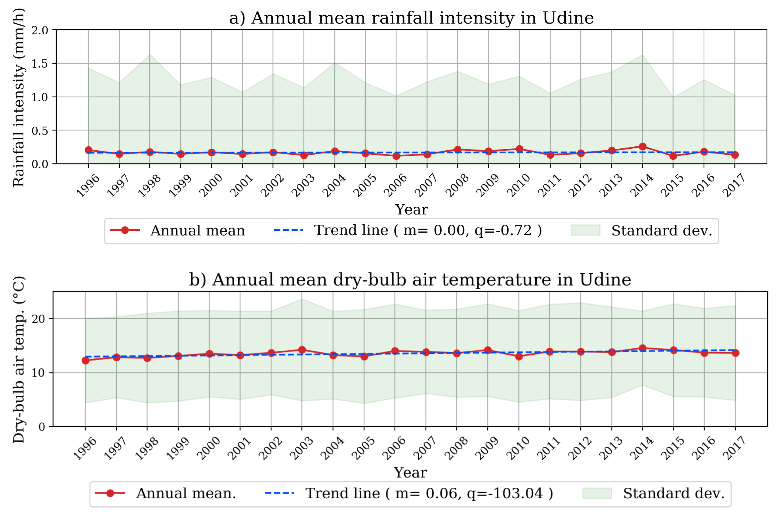
3.1. Weather Data Set
- n is the total number of hours in the considered year
- is the air dry-bulb temperature at hour h
- is the base temperature, set to 20 for the heating period and to 26 for the cooling period
- is the positive temperature difference for the calculation
- is the positive temperature difference for the calculation
3.2. Representative Years Evaluation Method
4. Results
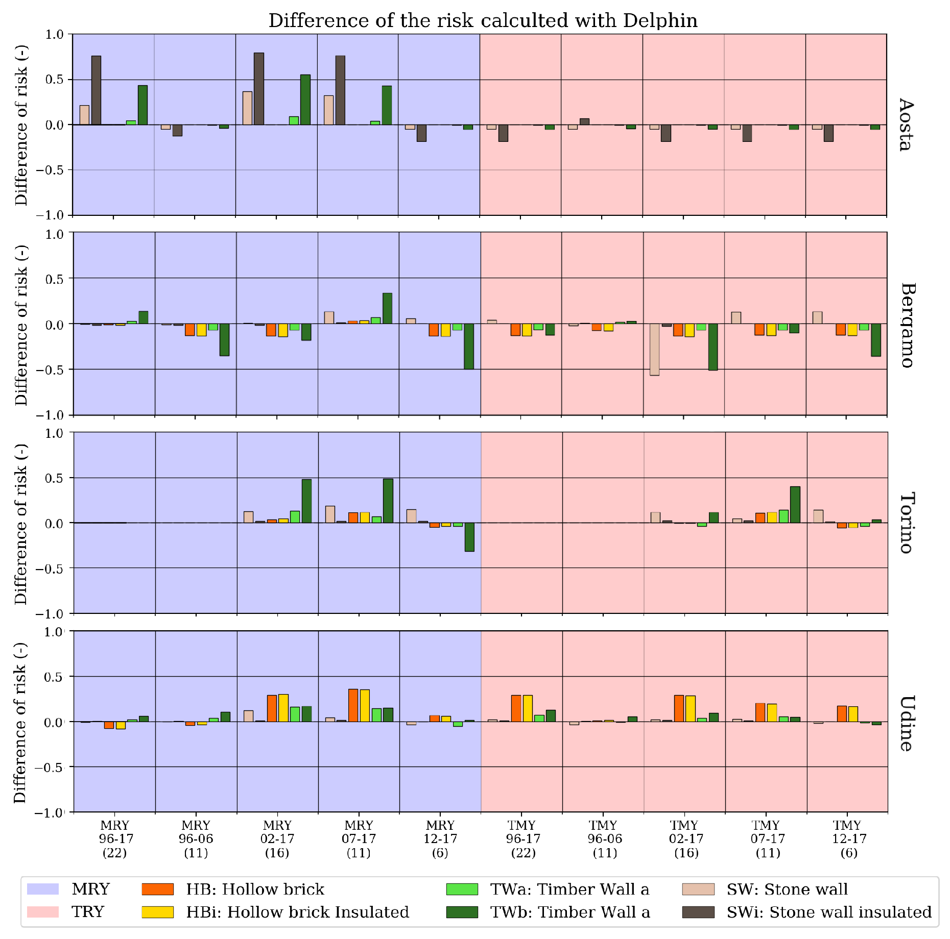
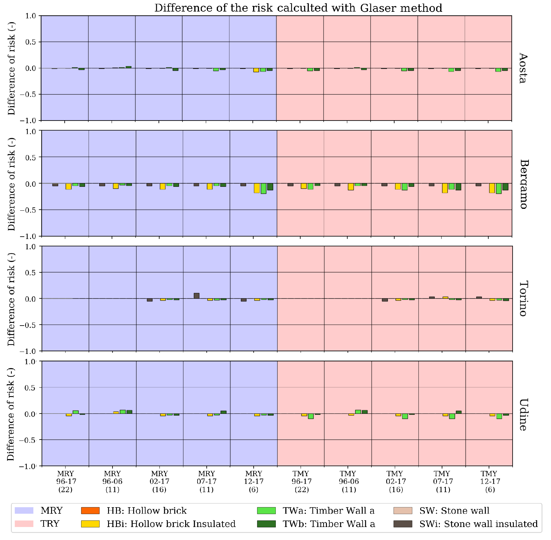
Risk Analysis
5. Conclusions
Author Contributions
Funding
Acknowledgments
Conflicts of Interest
References
- International Organization for Standardization. ISO 15927-4:2005. Hygrothermal Performance of Buildings—Calculation and Presentation of Climatic Data - Part 4: Hourly Data for Assessing the Annual Energy Use for Heating and Cooling (ISO 15927-4:2005); ISO: Geneva, Switzerland, 2005. [Google Scholar]
- Akkurt, G.; Aste, N.; Borderon, J.; Buda, A.; Calzolari, M.; Chung, D.; Costanzo, V.; Del Pero, C.; Evola, G.; Huerto-Cardenas, H.; et al. Dynamic thermal and hygrometric simulation of historical buildings: Critical factors and possible solutions. Renew. Sustain. Energy Rev. 2020, 118, 109509. [Google Scholar] [CrossRef]
- Rode, C.; Woloszyn, M. Whole-Building Hygrothermal Modeling in IEA Annex 41. In Proceedings—Thermal Performance of the Exterior Envelopes of Whole Buildings; American Society of Heating, Refrigerating and Air-Conditioning Engineers: Atlanta, GA, USA, 2007; pp. 1–15. [Google Scholar]
- Yang, J.; Fu, H.; Qin, M. Evaluation of Different Thermal Models in EnergyPlus for Calculating Moisture Effects on Building Energy Consumption in Different Climate Conditions. Procedia Eng. 2015, 121, 1635–1641. [Google Scholar] [CrossRef] [Green Version]
- Rode, C.; Grau, K. Synchronous calculation of transient hygrothermal conditions of indoor spaces and building envelopes. In Proceedings of the Building Simulation, Rio de Janeiro, Brazil, 13–16 August 2001; pp. 13–15. [Google Scholar]
- Rode, C. Combined Heat and Moisture Transfer in Building Constructions. Ph.D. Thesis, Thermal Insulation Laboratory, Technical University of Denmark, Lyngby, Denmark, 1990. [Google Scholar]
- Künzel, H.; Holm, A.; Zirkelbach, D.; Karagiozis, A. Simulation of indoor temperature and humidity conditions including hygrothermal interactions with the building envelope. Sol. Energy 2005, 78, 554–561. [Google Scholar] [CrossRef]
- Künzel, H.M. Simultaneous Heat and Moisture Transport in Building Components. Ph.D. Thesis, IRB-Verlag Stuttgart, Stuttgart, Germany, 1995. [Google Scholar]
- Libralato, M.; De Angelis, A.; Saro, O. Evaluation of the ground-coupled quasi-stationary heat transfer in buildings by means of an accurate and computationally efficient numerical approach and comparison with the ISO 13370 procedure. J. Build. Perform. Simul. 2019, 12, 719–727. [Google Scholar] [CrossRef]
- Rode, C.; Grau, K. Moisture Buffering and its Consequence in Whole Building Hygrothermal Modeling. J. Build. Phys. 2008, 31, 333–360. [Google Scholar] [CrossRef]
- Zhang, M.; Qin, M.; Rode, C.; Chen, Z. Moisture buffering phenomenon and its impact on building energy consumption. Appl. Therm. Eng. 2017, 124, 337–345. [Google Scholar] [CrossRef]
- Zu, K.; Qin, M.; Rode, C.; Libralato, M. Development of a moisture buffer value model (MBM) for indoor moisture prediction. Appl. Therm. Eng. 2020, 171, 115096. [Google Scholar] [CrossRef]
- De Angelis, A.; Saro, O.; Truant, M. Evaporative cooling systems to improve internal comfort in industrial buildings. Energy Procedia 2017, 126, 313–320. [Google Scholar] [CrossRef]
- De Angelis, A.; Medici, M.; Saro, O.; Lorenzini, G. Evaluation of evaporative cooling systems in industrial buildings. Int. J. Heat Technol. 2015, 33, 1–10. [Google Scholar] [CrossRef]
- De Angelis, A.; Ceccotti, L.; Saro, O. Energy savings evaluation for dry-cooler equipped plants in shopping mall buildings. Int. J. Heat Technol. 2017, 35, S361–S366. [Google Scholar] [CrossRef]
- De Angelis, A.; Ceccotti, L.; Saro, O. Cooling Energy Savings with Dry Cooler Equipped Plants in Office Buildings. Int. J. Heat Technol. 2016, 34, S205–S211. [Google Scholar] [CrossRef]
- De Angelis, A.; Chinese, D.; Saro, O. Free-cooling potential in shopping mall buildings with plants equipped by dry-coolers boosted with evaporative pads. Int. J. Heat Technol. 2017, 35, 853–862. [Google Scholar] [CrossRef]
- Italian Republic. Applicazione delle Metodologie di Calcolo delle Prestazioni Energetiche e Definizione delle Prescrizioni e dei Requisiti Minimi Degli Edifici; Ministerial Decree 26 June; Ministero dello Sviluppo Economico: Roma, Italy, 2016. (In Italian)
- International Organization for Standardization. ISO 13788:2012. Hygrothermal Performance of Building Components and Building Elements—Internal Surface Temperature to Avoid Critical Surface Humidity and Interstitial Condensation - Calculation Methods (ISO 13788:2012); ISO: Geneva, Switzerland, 2012. [Google Scholar]
- European Committee for Standardization. EN 15026. Hygrothermal performance of Building Components and Building Elements—Assessment of Moisture Transfer by Numerical Simulation (EN 15026:2007); CEN: Bruxelles, Belgium, 2007. [Google Scholar]
- International Organization for Standardization. ISO 15927-1:2003. Hygrothermal Performance of buildings—Calculation and Presentation of Climatic Data—Part 1: Monthly Means of Single Meteorological Elements (ISO 15927-1:2003); ISO: Geneva, Switzerland, 2003. [Google Scholar]
- Riva, G.; Murano, G.; Corrado, V.; Baggio, P.; Antonacci, G. Definizione degli anni Tipo Climatici delle Province di Alcune Regioni Italiane; ENEA Agenzia Nazionale per le Nuove Tecnologie, l’Energia e lo Sviluppo Economico Sostenibile: Roma, Italy, 2010; p. 347. (In Italian) [Google Scholar]
- Pernigotto, G.; Prada, A.; Gasparella, A.; Hensen, J.L. Analysis and improvement of the representativeness of EN ISO 15927-4 reference years for building energy simulation. J. Build. Perform. Simul. 2014, 7, 391–410. [Google Scholar] [CrossRef] [Green Version]
- Murano, G.; Dirutigliano, D.; Corrado, V. Improved procedure for the construction of a Typical Meteorological Year for assessing the energy need of a residential building. J. Build. Perform. Simul. 2018, 1–14. [Google Scholar] [CrossRef]
- Pernigotto, G.; Prada, A.; Cappelletti, F.; Gasparella, A. Impact of reference years on the outcome of multi-objective optimization for building energy refurbishment. Energies 2017, 10, 1925. [Google Scholar] [CrossRef] [Green Version]
- Kalamees, T.; Vinha, J. Estonian Climate Analysis for Selecting Moisture Reference Years for Hygrothermal Calculations. J. Build. Phys. 2004. [Google Scholar] [CrossRef]
- Zhou, X.; Derome, D.; Carmeliet, J. Robust moisture reference year methodology for hygrothermal simulations. Build. Environ. 2016, 110, 23–35. [Google Scholar] [CrossRef]
- Libralato, M.; Murano, G.; Saro, O.; De Angelis, A. Hygrothermal modelling of building enclosures: Reference year design for moisture accumulation and condensation risk assessment. In Proceedings of the 7th International Building Physics Conference, IBPC2018, Syracuse, NY, USA, 23–26 September 2018. [Google Scholar] [CrossRef]
- Lupato, G.; Manzan, M. Italian TRYs: New weather data impact on building energy simulations. Energy Build. 2019, 185, 287–303. [Google Scholar] [CrossRef]
- Finkelstein, J.M.; Schafer, R.E. Improved goodness-of-fit tests. Biometrika 1971, 58, 641. [Google Scholar] [CrossRef]
- Ente Nazionale Italiano di Unificazione. UNI 10349:2016. Riscaldamento e Raffrescamento degli Edifici—Dati Climatici - Parte 3: Differenze di Temperatura Cumulate (Gradi Giorno) ed altri Indici Sintetici (UNI 10349:2016); UNI: Rome, Italy, 2016. (In Italian) [Google Scholar]
- Sontag, L.; Nicolai, A.; Vogelsang, S. Validierung der Solverimplementierung des Hygrothermischen Simulationsprogramms Delphin; Saechsische Landesbibliothek-Staats-und Universitaetsbibliothek Dresden: Dresden, Germany, 2013. [Google Scholar]
- Ballarini, I.; Corgnati, S.P.; Corrado, V. Use of reference buildings to assess the energy saving potentials of the residential building stock: The experience of TABULA project. Energy Policy 2014, 68, 273–284. [Google Scholar] [CrossRef]
- D’Amico, A.; Ciulla, G.; Panno, D.; Ferrari, S. Building energy demand assessment through heating degree days: The importance of a climatic dataset. Appl. Energy 2019, 242, 1285–1306. [Google Scholar] [CrossRef]
- D’Agaro, P.; Coppola, M.; Cortella, G. Field tests, model validation and performance of a CO2 commercial refrigeration plant integrated with HVAC system. Int. J. Refrig. 2019, 100, 380–391. [Google Scholar] [CrossRef]
- Coccia, G.; D’Agaro, P.; Cortella, G.; Polonara, F.; Arteconi, A. Demand side management analysis of a supermarket integrated HVAC, refrigeration and water loop heat pump system. Appl. Therm. Eng. 2019, 152, 543–550. [Google Scholar] [CrossRef]
- Cortella, G.; D’Agaro, P.; Coppola, M. Transcritical CO2 commercial refrigeration plant with adiabatic gas cooler and subcooling via HVAC: Field tests and modelling. Int. J. Refrig. 2020, 111, 71–80. [Google Scholar] [CrossRef]
- Santin, M.; Chinese, D.; Saro, O.; De Angelis, A.; Zugliano, A. Carbon and Water Footprint of Energy Saving Options for the Air Conditioning of Electric Cabins at Industrial Sites. Energies 2019, 12, 3627. [Google Scholar] [CrossRef] [Green Version]
- Chinese, D.; Santin, M.; Saro, O. Water-energy and GHG nexus assessment of alternative heat recovery options in industry: A case study on electric steelmaking in Europe. Energy 2017, 141, 2670–2687. [Google Scholar] [CrossRef] [Green Version]


| Station | Lat. | Long. | Alt. | MY Years |
|---|---|---|---|---|
| () | () | (m a.s.l.) | ||
| Aosta—Saint-Christophe | 45.75 | 7.68 | 569 | 1996–2017 |
| Bergamo—via Stezzano | 45.66 | 9.66 | 211 | 1996–2017 |
| Torino—Loc. Bauducchi | 44.96 | 7.71 | 226 | 2002–2017 |
| Udine—S. Osvaldo | 46.03 | 13.23 | 91 | 1996–2017 |
| Station | T | x | ||||
|---|---|---|---|---|---|---|
| () | (g/kg) | (g/kg) | (Degree Days) | (Degree Days) | (mm/year) | |
| Aosta | 11 | 5.3 | 4.6 | 3493 | 66 | 563 |
| Bergamo | 13 | 7.5 | 3.6 | 2813 | 94 | 1173 |
| Torino | 13 | 7.4 | 3.4 | 3099 | 102 | 757 |
| Udine | 13 | 7.6 | 3.4 | 2760 | 83 | 1485 |
| Station | T | x | ||||
|---|---|---|---|---|---|---|
| () | (g/kg) | (g/kg) | (Degree Days) | (Degree Days) | (mm/year) | |
| Aosta | 12 | 5.6 | 4.7 | 3378 | 101 | 454 |
| Bergamo | 14 | 7.4 | 4.5 | 2629 | 141 | 1181 |
| Torino | 13 | 7.7 | 3.4 | 3066 | 122 | 590 |
| Udine | 14 | 8.1 | 3.9 | 2656 | 106 | 1400 |
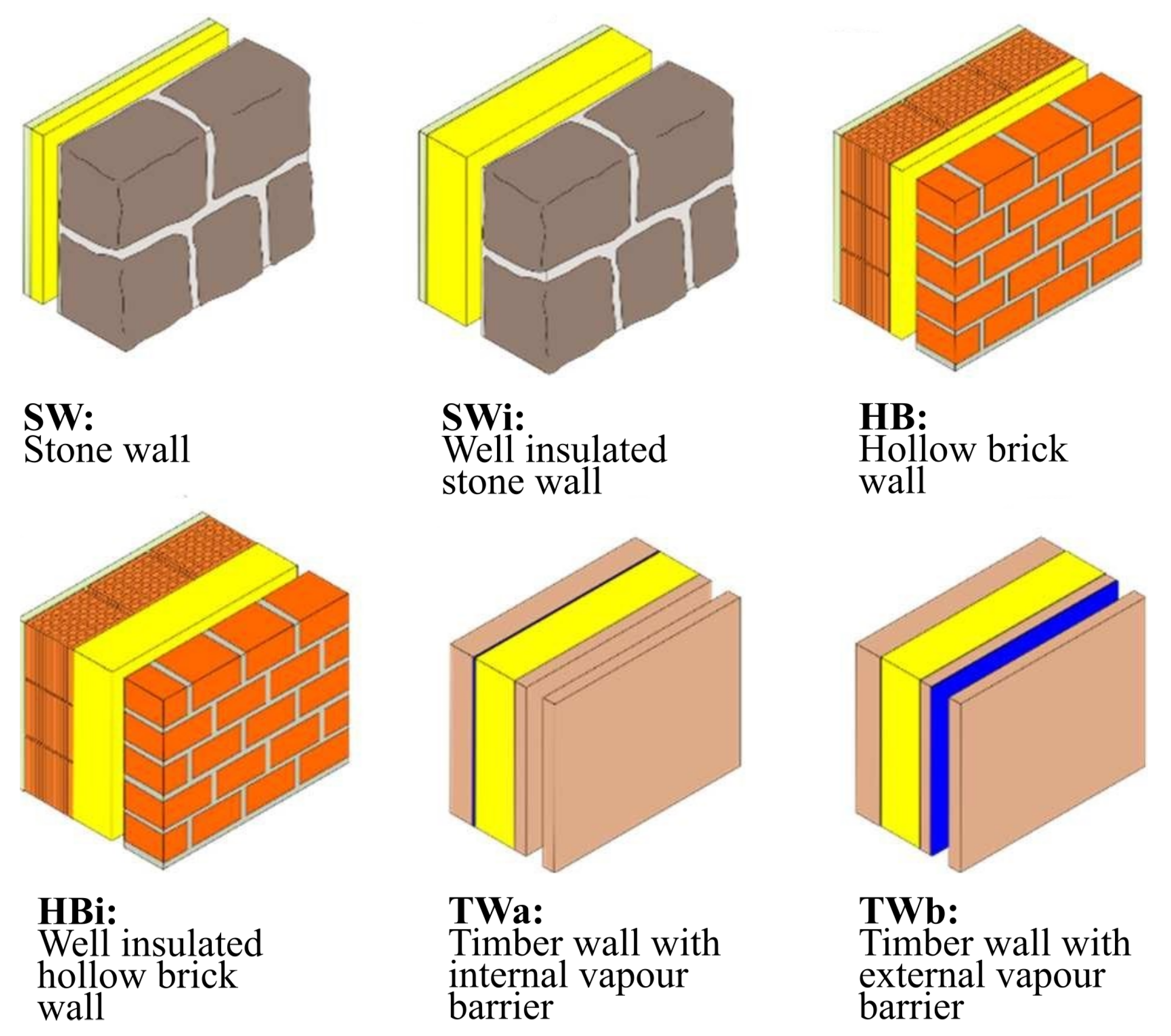
| Wall | Id. | d | U | |
|---|---|---|---|---|
| (m) | (W/mK) | (m) | ||
| Stone wall | SW | 0.38 | 0.70 | 5 |
| Well insulated stone wall | SWi | 0.53 | 0.13 | 50 |
| Hollow brick wall | HB | 0.49 | 0.39 | 7 |
| Well insulated hollow brick wall | HBi | 0.58 | 0.15 | 41 |
| Timber wall with internal vapour barrier | TWa | 0.53 | 0.13 | 56 |
| Timber wall with external vapour barrier | TWb | 0.53 | 0.13 | 56 |
© 2020 by the authors. Licensee MDPI, Basel, Switzerland. This article is an open access article distributed under the terms and conditions of the Creative Commons Attribution (CC BY) license (http://creativecommons.org/licenses/by/4.0/).
Share and Cite
Libralato, M.; Murano, G.; De Angelis, A.; Saro, O.; Corrado, V. Influence of the Meteorological Record Length on the Generation of Representative Weather Files. Energies 2020, 13, 2103. https://0-doi-org.brum.beds.ac.uk/10.3390/en13082103
Libralato M, Murano G, De Angelis A, Saro O, Corrado V. Influence of the Meteorological Record Length on the Generation of Representative Weather Files. Energies. 2020; 13(8):2103. https://0-doi-org.brum.beds.ac.uk/10.3390/en13082103
Chicago/Turabian StyleLibralato, Michele, Giovanni Murano, Alessandra De Angelis, Onorio Saro, and Vincenzo Corrado. 2020. "Influence of the Meteorological Record Length on the Generation of Representative Weather Files" Energies 13, no. 8: 2103. https://0-doi-org.brum.beds.ac.uk/10.3390/en13082103