Electrical Faults Signals Restoring Based on Compressed Sensing Techniques


Electrical Engineering, Universidad Politécnica Salesiana, Quito EC170146, Ecuador
*
Author to whom correspondence should be addressed.
Energies 2020, 13(8), 2121; https://0-doi-org.brum.beds.ac.uk/10.3390/en13082121
Submission received: 17 March 2020
/
Revised: 20 April 2020
/
Accepted: 21 April 2020
/
Published: 24 April 2020
(This article belongs to the Section F: Electrical Engineering)
Abstract
:This research focuses on restoring signals caused by power failures in transmission lines using the basis pursuit, matching pursuit, and orthogonal matching pursuit sensing techniques. The original signal corresponds to the instantaneous current and voltage values of the electrical power system. The heuristic known as brute force is used to find the quasi-optimal number of atoms k in the original signal. Next, we search for the minimum number of samples known as m; this value is necessary to reconstruct the original signal from sparse and random samples. Once the values of k and m have been identified, the signal restoration is performed by sampling sparse and random data at other bus bars of the power electrical system. Basis pursuit allows recovering the original signal from 70% of the random samples of the same signal. The higher the number of samples, the longer the restoration times, approximately 12 s for recovering the entire signal. Matching pursuit allows recovering the same percentage, but with the lowest restoration time. Finally, orthogonal matching pursuit recovers a slightly lower percentage with a higher number of samples with a significant increase in its recovery time. Therefore, for real-time electrical fault signal restoration applications, the best selection will be matching pursuit due to the fact that it presents the lowest machine time, but requires more samples compared with orthogonal matching pursuit. Basis pursuit and orthogonal matching pursuit require fewer sparse and random samples despite the fact that these require a longer processing time for signal recovery. These two techniques can be used to reduce the volume of data that is stored by phasor measurement systems.
1. Introduction
The electrical Power System (PS) is one of the most complex networks in the world; it is an interconnected grid established by generation units, substations, transmission, distribution lines, and loads. The diagnosis of failures in electrical power systems through Signal Processing (SP) is applied to the Power Quality (PQ) associated with the implementation of Smart Grid (SG) technologies. The increasing complexity of the electric grid requires signal processing in order to characterize, identify, and diagnose the system behavior accurately [1,2].
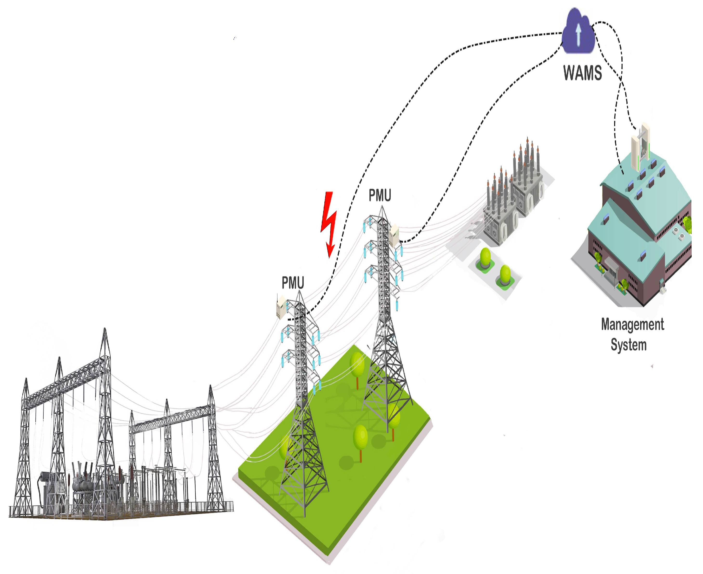
The detection of an event, in electrical power systems, is the basis for carrying out numerous applications in the safety, power quality monitoring, analysis, and control systems fields. It is important to say that the device which is going to be on charge of detecting and evaluating the events that present any type of disturbance or distortion in a electrical system, must be as thorough as possible when evaluating an anomaly in the system, since a poor performance of this device can result in a false alarms on events that are not important [3]. This aim most of the time is not achieved due to the fact that the processed data are so big that the equipment is not able to react on time. As can be seen in Figure 1, currently, the process to transform analog signals to digital signals is carried out by several secondary smart digital devices knows as Phasor Measurement Unit (PMU) that perform the task of controlling, metering, protecting, supervising, and communicating with other modules of the system. The large amount of data that is acquired by sensors installed in the different points of the electricity network consume large amounts of energy, which is necessary to process information as a consequence of the large volume of data traffic [4].
The quality of smart devices is determined by their ability to perform Digital Signal Processing (DSP) using mathematics, algorithms, and techniques to manipulate signals [5,6]. Lets suppose that a it is intended to monitor the energy quality of our system, here there are several elements that are part in the monitoring and measurement process; however, definitively one of the most important is the device that is in charge of detecting the failures of the electrical network. This multifunctional element is available to record real-time events that will be used for future analysis, it also can classify the elements according to their characteristics. In the first case, if a false alarm occurs in the presence of a minor event, this could lead that irrelevant information could saturate the memory space. On the other hand, if the device is not precise enough, an important event could not be detected and the information would simply be lost. As a result of these two scenarios, a new theory known as compressed sensing is applied with the aim of reducing information by cutting the number of samples required to reconstruct the original data. Therefore, using the same idea, the proposal is to minimize the amount of data required to rebuild the original signal needed to recognize and classify a fault or non-fault detection of any device [7].
Recently, particularly high interest has been seen in signal processing, especially how to sample and compress these signals. Because of the desire to process the signal and in particular achieve a higher quality of the acquired signal and obtain a high performance in data compression, some models have been developed that propose that a signal considered dispersed can be efficiently represented or reconstructed from a small set of measurements [8]. The lower number of the sample frequency of the signal is directly related to the decrease in energy consumption and especially the optimization of computational time to process that signal. It is important to say that, due to the advantages of this methodology, it has a very wide application range, especially in devices that have low resolution or in equipment that requires extremely high sampling frequencies.
There are several techniques that can be used for signal reconstruction, but this article will focus on the most relevant, compressed sensing [9]. The main aim of this methodology is that any type of signal can be represented approximated by a sparse signal; that is to say, an input signal can be characterized by a linear combination composed of its most significant terms. Thus, it can be said that compressed sensing is a promising technology, which will contribute to the significant development of the way in which signal processing is currently performed, reducing computational costs and thus optimizing the use of other resources such as energy [10]. Compressed sensing is a versatile tool, which can be applied in several situations. For instance, one case is a small sample set that is a direct consequence of the lack of physical availability. A second case is a study in which the large amount of information collected does not allow the fast processing of such information, and it needs to be reduced to its most significant samples without compromising all the information. In addition, a third case is that the access to the amount of data collected is affected or prohibited by the presence of noise.
Lately, numerous studies have been developed on sparse signal reconstruction, for example a complete analysis of a the orthogonal matching pursuit algorithm technique was presented in [11]. It is an alternative and optimized approach initially posed by the Nyquist–Shannon theorem and based on the fact that a small number of non-adaptive linear projections on a compressible signal contains enough information to rebuild and process it. However, this approach was done for an audio signal. Both Chretien [12] and Tropp [13] provided an extensive and comprehensive report about matching pursuit. The first one used MP to decompose a signal in a linear expansion of waveforms that were selected from a redundant dictionary of functions, which was simply the resulting matrix after applying a transform to the input signal. In this paper, the transform was based on the Gabor function that defines an adaptive time-frequency transform. The second one used alternative methods for the lo-norm. The difference is due to its discrete and discontinuous nature; this theorem does not satisfy all mathematical axioms, since it is simply not a norm. This theorem is based on the total number of nonzero elements in a vector. There are also authors who complement compressed sensing with probabilistic techniques, such as the Bayesian approach. It can be seen as an extension of propositional logic that allows reasoning with propositions whose truthfulness or falseness are uncertain [14].
In contrast, this paper integrates all the basic considerations used by utilities to obtain the best option to reconstruct a sparse signal. It is known that electricity demand is rising, and it is a priority to find new solutions that allow reducing the maintenance and operation costs of the electrical system in a safe and reliable way. Set in this context, fault detection in an electrical system and processing the signal are extremely important in order to meet this objective. Consequently, the proposed algorithm analyzes several methodologies in which a fault signal can be reconstructed, from a few samples, to obtain an accurate selection to process that signal. Additionally, the methodology suggested in this paper can be used in real-life situations and not only as a technical simulation; therefore, the reconstruction of fault signals from a few sampled signals can be useful for academic and practical purposes [15].
2. Compressed Sensing Theory
The ability to detect an electrical signal, under fault conditions, is widely in electrical systems not only for monitoring the event but also for taking preventive actions in order to protect the system. It extremely important that the system separates the difference between a failure event and an event that does not deserve to be considered as a fault, thus it is possible to select exclusively the events that represent a risk for the system and discard events that present false and unimportant information. This characteristic is extremely important since a false reading of the device will lead, in many cases, in the lack of energy along an electrical line that does not present any error at all. At the moment the device detects a fault, it will be able to classify the fault according to the parameters required and previously pre-established by the user. On the other hand, if the device is not capable of identifying a fault that may be critical to the system, the consequences will be catastrophic not only for the system but also for the consumer, because this would lead to a total blackout.
Compressive sensing is an alternative technique for Shannon/Nyquist sampling [16], for reconstruction of a sparse signal that can be well recovered by just components from an basis matrix. For this, x should be sparse, that is to say it must have k different elements from zero where . This technique is used to recover a sparse-enough signal from a small number of measurements [17].
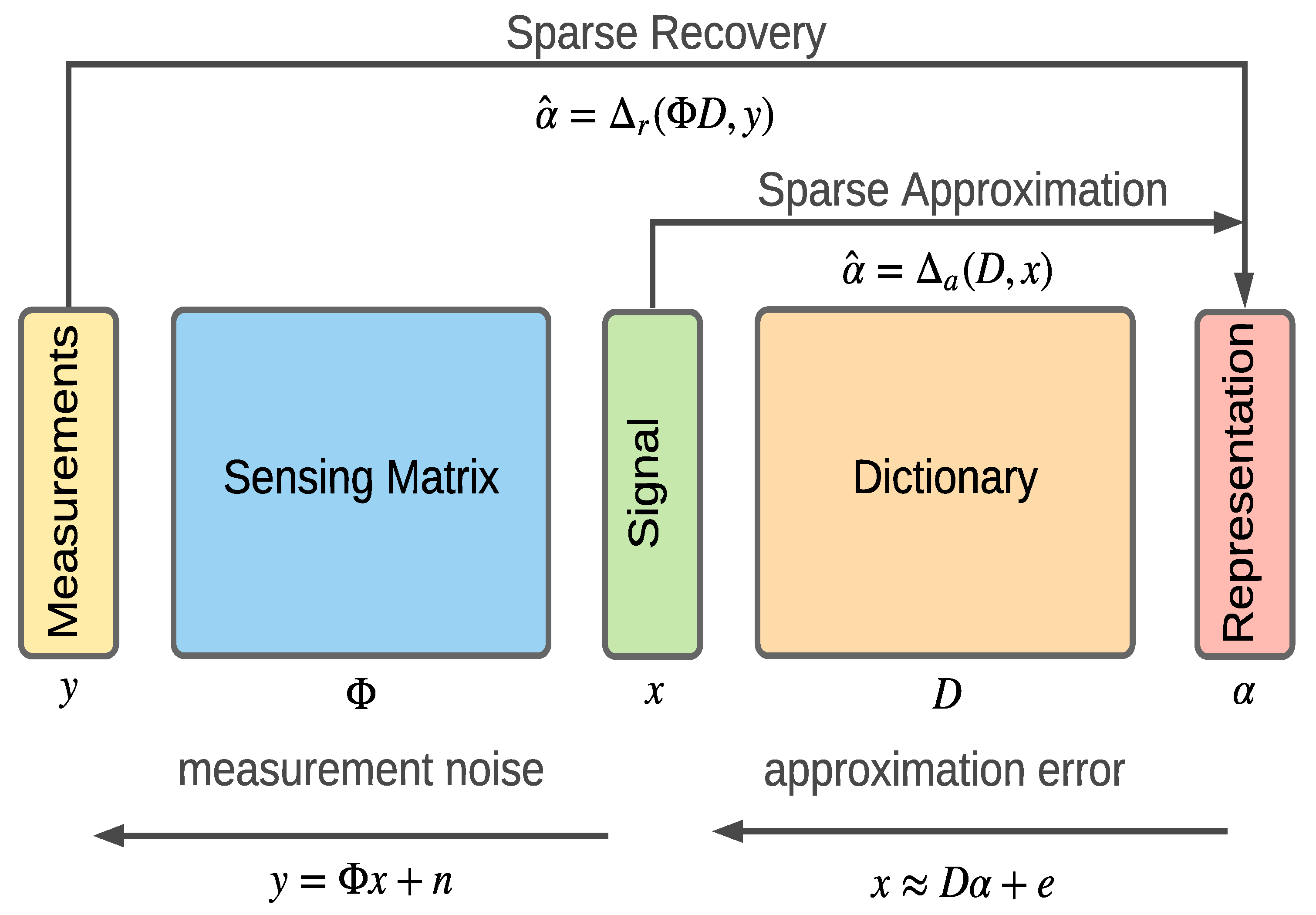
Electrical fault signals have a sparse representation and could be compressed using the framework of sensing shown in Figure 2. Signals are located in a memory spot called . The registers can be configured as the signals located there do not have a significant representation within that and thus this infromation representations can have its own memory space . An algorithm is able to create a description for a signal x in the dictionary D. There is also an error represented by e. However, a little quantity of samples is not enough to determinate the information needed by x. The sensing process create information which can be put together in a vector for a given signal where the existing noise at the measurement process is n. X can be obtained from y, if we obtain the sparse representation by using the sparse recovery algorithm . Finally, [17].
The following equation, which is a matrix expression, is a common definition which represent a typical generic sparse acquisition problem.
where:
- y is the acquired sample vector of dimension [M × 1];
- is the sensing matrix of dimension [M × N];
- is the sparse signal representation of dimension [N × 1];
- n is the additive noise contribution of dimension [N × 1].
To represent a signal with compressive sensing, it is necessary to obtain the dictionary matrix, D, which may be constructed by different elementary waveforms generated from a variety of basic functions, such as Short-Time Fourier Transform (STFT), Wavelet Transform (WT), Discrete Cosine Transform (DCT), Hilbert Transform (HT), Gabor Transform (GT), the Wigner Distribution Function (WDF), S-Transform (ST), Gabor–Wigner Transform (GWT), Hilbert–Haung Transform (HHT), and hybrid transform based methods.
2.1. Restricted Isometry Property
The incoherence criterion relies on the assumption that the signal x admits a k-sparse representation y in a given sparsifying domain. However, in practice, this knowledge is unavailable a priori. The aforementioned decomposition into a sensing and sparsifying matrix is no longer feasible, and the sensing matrix has to be taken into account as a whole
The best way in which the inconsistency criterion could be explained is that given a dispersion domain, there is a signal x which admits another signal y with a k—dispersed representation. Despite the fact that in practice this knowledge is not well developed, it is known that the information previously described can be decomposed into two matrices: a dispersion matrix and a detection matrix which must be considered in its whole domain.
First a signal x must be assumed which is k-sparse or k-compressible in D and . The aim is to obtain x starting from another signal y considering that and D are values which are already known. The process explined previously can be archived by obtaining the sparse representation from y so later we can calculate .
A bad scenario could be the possibility that k-column submatrices of are not well conditioned, so there is a chance that some sparse signals get mapped to very similar measurement vectors. Hence, it is not stable to reconstruct the signal mathematically. Furthermore, if any kind of noise or disturbance is present during the process, the veracity of the process decreases even more [20]. The two authors Candes and Tao describe that due to the nature of a sparse signals, it must be conserved according the action of a sensing matrix. Especially, you have to keep in mind that the space between two sparse signals must be regardless of any disturbances that may exist [21]. Both authors developed this criteria and represented it in the form of a matrix where the the smallest number is for which the following holds:
When , the Equation (3) implies that each collection of k columns from is non-singular. As it is desire that every collection of 2k columns to be non-singular, the value of is needed, which is the minimum requirement for the recovery of k sparse signals.
Additionally, if , it is important to notice that the sensing operator very nearly maintains the l2 distance between any two k sparse signals. As a result of this, invert the sensing process stably is possible.
At this point, it is clear the fact that many randomly generated matrices have excellent RIP performance. It is possible to show that if , then with measurements, the probability to recover x is very high.
2.2. Minimum Norm Solution
norm: In the CS context, it is necessary that will be sparse. The solution presented as follow is a commun representation for the solution recovery:
norm: Assuming a matrix A which satisfy RIP criterion, highly sparse solutions can be obtained by convex optimization. In such a way, the algorithm is commonly know as Basis Pursuit (BP): [22,23].
The problematic present can be recognise as a recovery problem which can be define as a convex optimization. A efficient solution to this problem will be throughout linear programming techniques using a canonical simplex method or the more recent interior point method.
norm: This method is commonly known as the Least Squares (LS) solution, and it aim is to minimize the residual energy in order to ensure adjust data resulting from measurement [24].
2.3. Matching Pursuit
This is also an algorithm (Algorithm 1) which develop an sparse approximation in order to obtain the “best matching” projections of multidimensional data onto the span of an over-complete dictionary D. This means that a signal f cab be represent starting from Hilbert space H approximately as the weighted sum of finitely many functions (called atoms) taken from D [25].
| Algorithm 1: Matching Pursuit [17]. |
| Input: Signal: , dictionary D with normalized columns |
| Output: List of coefficients and indices for corresponding atoms |
| Initialization: |
| Repeat: |
| Find with maximum inner product ; |
| ; |
| ; |
| ; |
| Until stopping condition (for example: ) |
| return |
2.4. Orthogonal Matching Pursuit
The aim of this method is to collect enough information to reconstruct a sparse vector from the process of identify the vector of indices ȷ composed by , so that the columns of are selected accurately in order to minimize the cardinality of the error of the signal compressed in the MDMSand the approximation . In OMP, the amplitude of the atoms most of the time is orthogonal to the residue, this amplitude is named . Thus the found vector ȷ consist of the index . The following equation explains how to solve this problem.
OMP is an ambitious algorithm (Algorithm 2) since it starts by determining the largest atoms of ; and it is also based on matching pursuit. Nevertheless, this work does not expose the characteristics of this algorithm since it was not implemented due to the limitations it contains regarding the increase of the number of iterations [20,26,27].
| Algorithm 2: Orthogonal Matching Pursuit [20]. |
| Input: Measurement matrix A , observed vector y , sparsity k |
| Initialization: |
| for i |
| with maximum inner product ; |
| ; |
| ; |
| ; |
| Until stopping condition (for example: ) |
| return |
2.5. Basis Pursuit
This is another algorithm (Algorithm 3) that can considered as a mathematical optimization problem, the equation which explain this method is presented below.
where x is an solution vector which will be the signal, y is an vector of observations which represent the measurements, is an transform matrix which is usually the measurement matrix, and finally it must to be considered that . This algorithm is commonly used in scenarios where exist an underdetermined system of linear equations such as , this equation must to be totally satisfied, and the sparsest solution in the sense is desired [28].
| Algorithm 3: Basis Pursuit [28]. |
| Input: |
| Procedure: |
| such that and |
| indices corresponding to the k largest magnitude entries in |
| such that and |
| Output: x and T |
3. Problem Formulation
The fact that a sparse signal can be recovered, with high probability, from a small set of random linear projections using nonlinear reconstruction algorithms, has a high level of applicability within several engineering fields. The signal can be sparse in the time or frequency domain, and the number of random projections used to recover the signal, in general, is much less than the number of samples, allowing reducing the sampling frequency and thus also decreasing the analog-to-digital conversion resources, storage resources, and transmission resources. Not many works have been published on the potential of using this theory; however, algorithms such as matching pursuit, orthogonal matching pursuit, and basis pursuit allow developing practical and implementable applications such as fault detection in a power electrical system.
In the new scenario of smart grids, more signal processing methods for electrical parameters are required to keep the network under control and operate at the desired quality of service and reliability. For this purpose, electrical parameters in terms of voltage, current signals considering the magnitude, phase, and waveforms are studied from a more complex point of view where the new frequency components add higher variations that affect measurement parameters. Moreover, monitoring the all the system parameters at every location requires high performance tools for state estimation of system parameters. As a result, the estimation and further processing of electrical power system parameters become an essential feature of power system analysis [29].
The complexity of the electrical grid will require not only advanced signal processing that can identify specific parameters, but also intelligent methods that identify the behavioral patterns of the system under fault conditions. There are no previous studies or comparative analyses of how compressed sensing can be used to detect faults in electric power systems [15,25].
A dual detection problem can be analyzed by two hypotheses. The first one is related to the assumption that a fault occurs; for instance, a short circuit between two phases of the electrical power system. The second one is associated with the supposition that a fault event does not occur; for example, a system is under normal operation. The statistical properties of the hypotheses are usually very complex or unknown. In order to have a better understanding of the process of the signals in either of these situations, techniques such a compressed sensing can be implemented. Compressed sensing is an alternative technique to Nyquist–Shannon sampling, for reconstruction of a sparse signal that can be well recovered by just components from an basis matrix. For this, x should be sparse, that is to say that it must have k different elements from zero where . This technique is used to recover a sparse-enough signal from a small number of measurements.
The technical and economic aspect is also considered, since it is not possible to install measurement sensors along the entire PS; hence, using the concept of the sparse matrix, in which there will be few points where the measurement equipment can be located, a sparse matrix is created from the measurements obtained along the electrical system. In addition, using the concept of compressed sensing, it is projected to find the points at which to locate the measurement equipment under the optimization criteria.
There are some studies on the behavior of communications networks for the transmission of data obtained from the sensors under the Nyquist–Shannon sampling theory [27,30]. According to the information obtained, it has been possible to detect and classify different types of events on transmission lines in electric power systems. First, full access to all the data that arrive at a bus bar due to a fault event has to be assumed. Applying signal processing techniques, a dictionary is found that represents the signal based on the orthonormal bases. The present research focuses on the establishment of the optimal sampling points of the signals under the establishment of the correct dictionary and the use of the and standard under the RIP restrictions and compressed sensing.
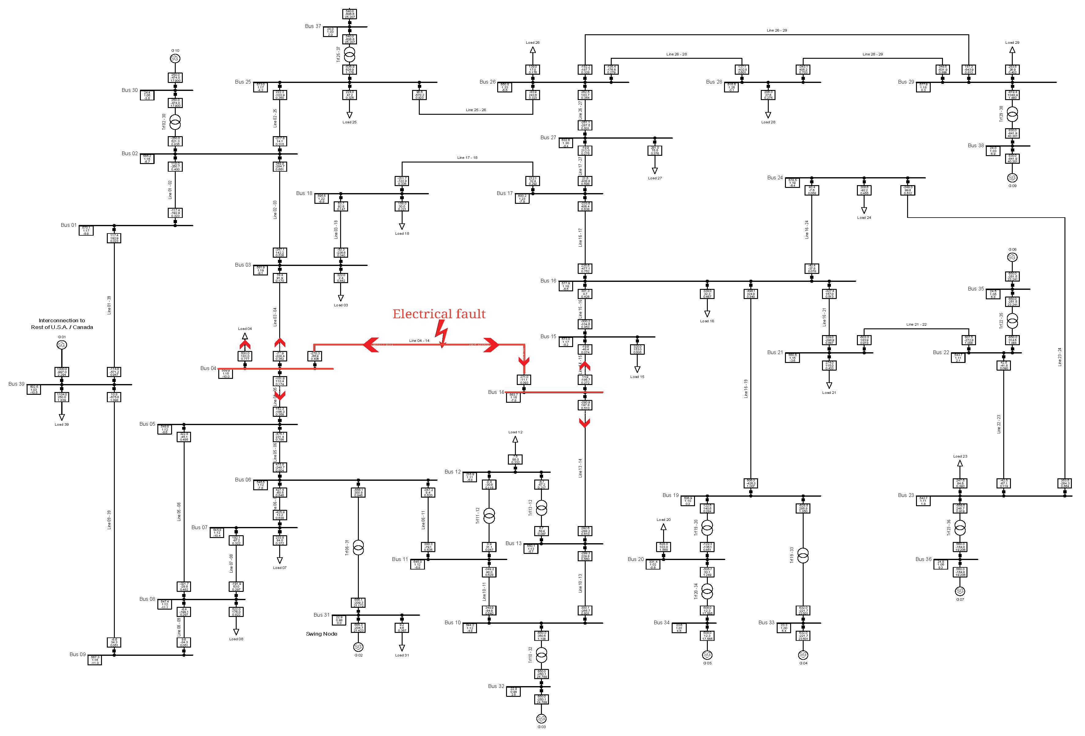
For the present study, the IEEE 39-bar model was taken as a case study. This is a model that shows the arrangement of a transmission line, and it is widely used in the study of electrical flows and fault analysis as well. A fault in a circuit is any event that interferes with the normal flow of current. Most transmission line failures are caused by lightning strikes that result in opening insulators [31]. The high voltage between a conductor and the grounded tower that supports it causes ionization, which provides a path to the ground for an atmospheric discharge. Additionally, opening the switches, to isolate the failed portion of the line from the rest of the system, interrupts current flow in the ionized path and allows deionization in the circuit [32]. Generally, in transmission line operation, a re-connection of the switches is highly successful after a fault. In Figure 3, the red line shows the presence of a fault; this event will generate several post fault voltage and current signals that will be used later as the base of the signal reconstruction. In order to investigate all the possibilities, the 11 types of failures that could occur in transmission lines were simulated; as consequence, it was verified that the results obtained and validated in a three-phase fault included the signals of the remaining 10 types of failures. The three-phase fault produced an electromagnetic phenomena that could be evidenced in the current and voltage signals that were recorded by the PMU at both ends.
4. Analysis and Results
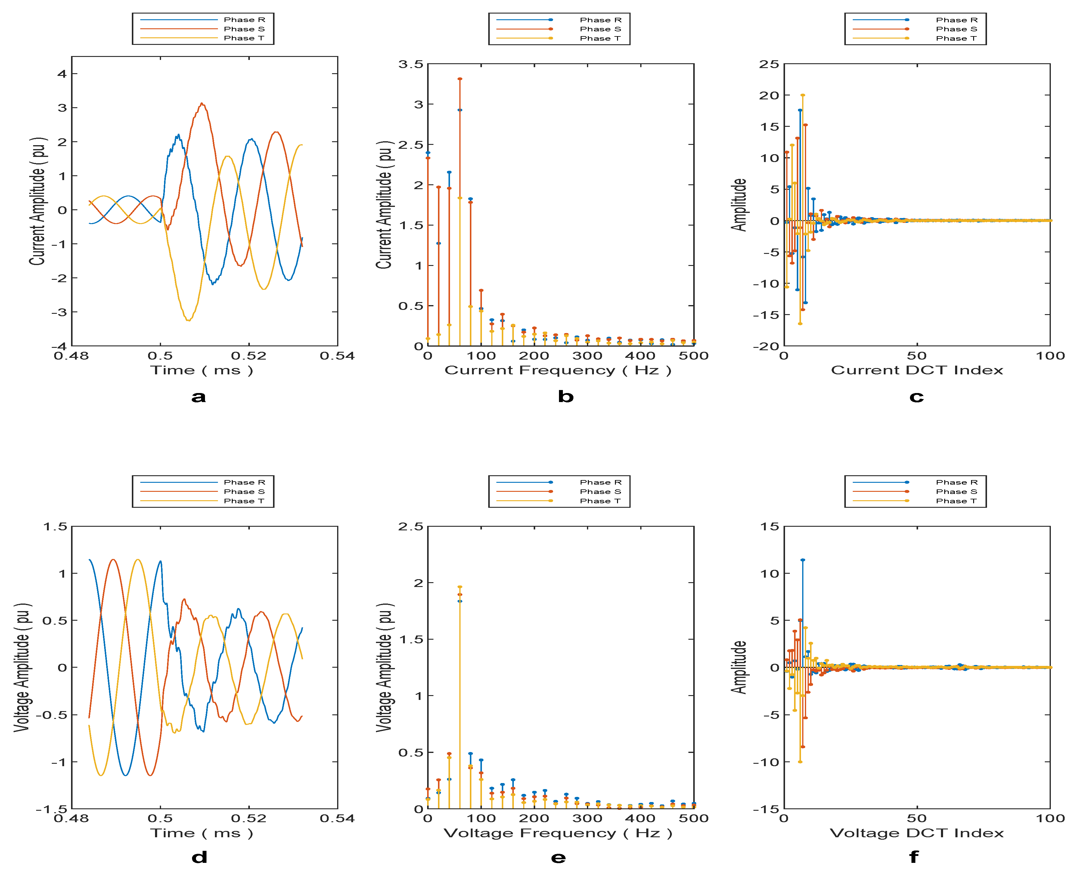
In Figure 4, top left corner, the three-phase current signals in Bus 4 are shown, presenting that there is a phase and magnitude disturbance. The frequency spectrum that is the result of the electrical fault is shown in Figure 4, top center. In this figure, the frequency with greater amplitude is the fundamental one of 60 Hz; however, new frequency components have been included due to the electrical failure. In Figure 4d, the voltage signal presents phase disturbances and a magnitude decrease. The frequency spectrum that is the result of electrical fault is shown in Part e. In this figure, also the frequency with greater amplitude is the fundamental one of 60 Hz; however, new frequency components have been included due to the electrical failure. In Part f, the discrete cosine transform is shown. It can be seen that the energy of the signal is concentrated in a few data, allowing us to create a sparse matrix.
4.1. Matching Pursuit Results
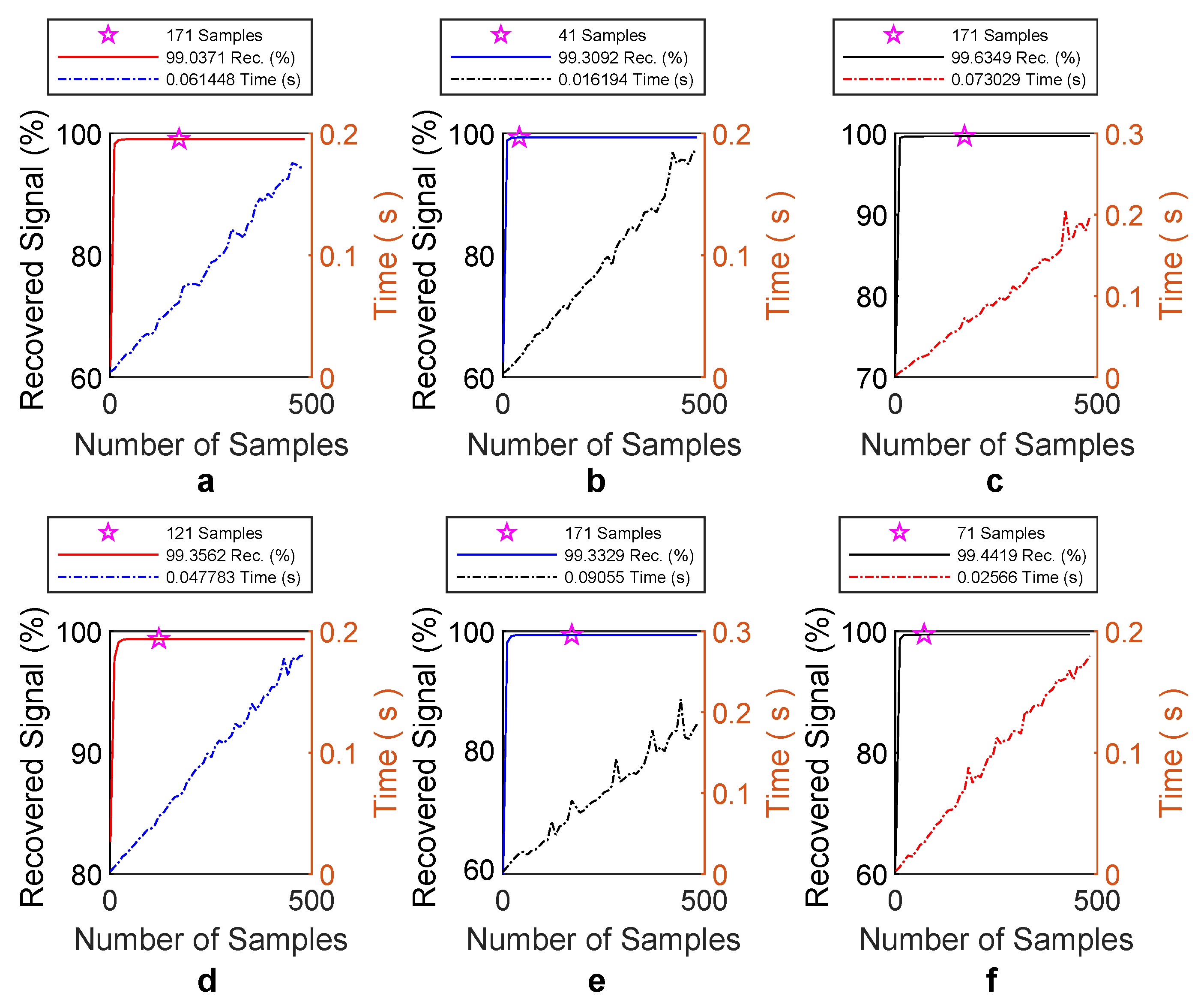
To solve the problem of signal restoration using the matching pursuit model, first, it is necessary to establish the number of atoms in the signal known as k. The atoms of the signal are the minimum number of samples that represent the entire signal. Figure 5 shows the optimal number k signal atoms of the signal under fault conditions; thus, the number of random samples needed by the atoms is 171 for a fault signal with no noise. As can be seen, the execution time of the algorithm to find the optimal value of k is less than 0.2 s.
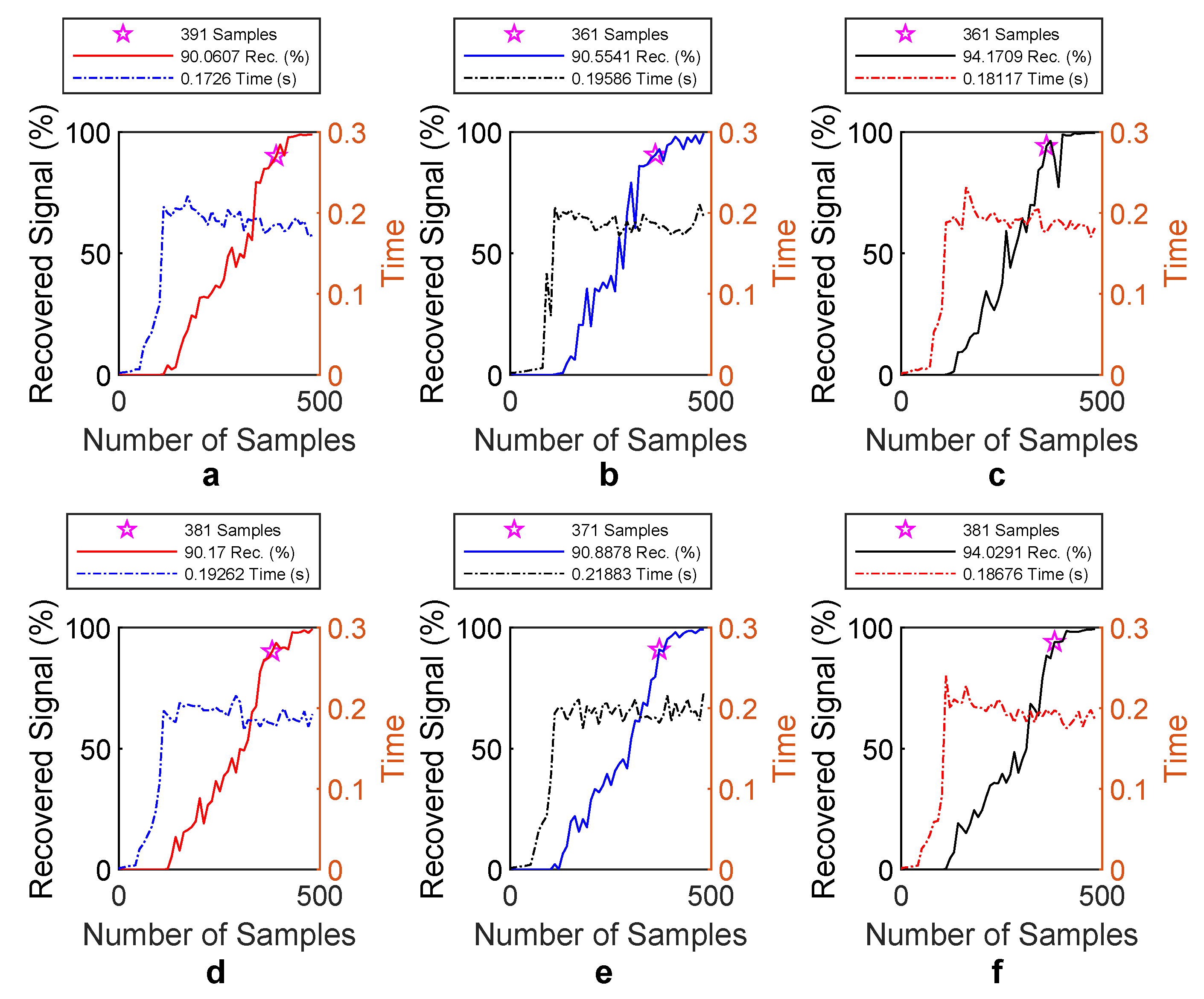
Second, the number of samples needed to reconstruct the signal will be calculated. Figure 6 shows the number of samples needed to reconstruct 90% of the signal as a function of the original one. The scenario with the highest number is Part a. It requires 391 random samples of the original signal, which is equivalent to 80% of the original signal data, and the machine time required to process the algorithm is 0.1726 s.
Finally, once the number of samples is calculated, the optimal values in order to reconstruct the signals can be obtained. For this case, k = 171, which corresponds to 35% of the base signal, and m = 391, corresponding to 80% of the same one. Next, the reconstruction tests of the signals produced by the electrical failures are developed at Bar 14.
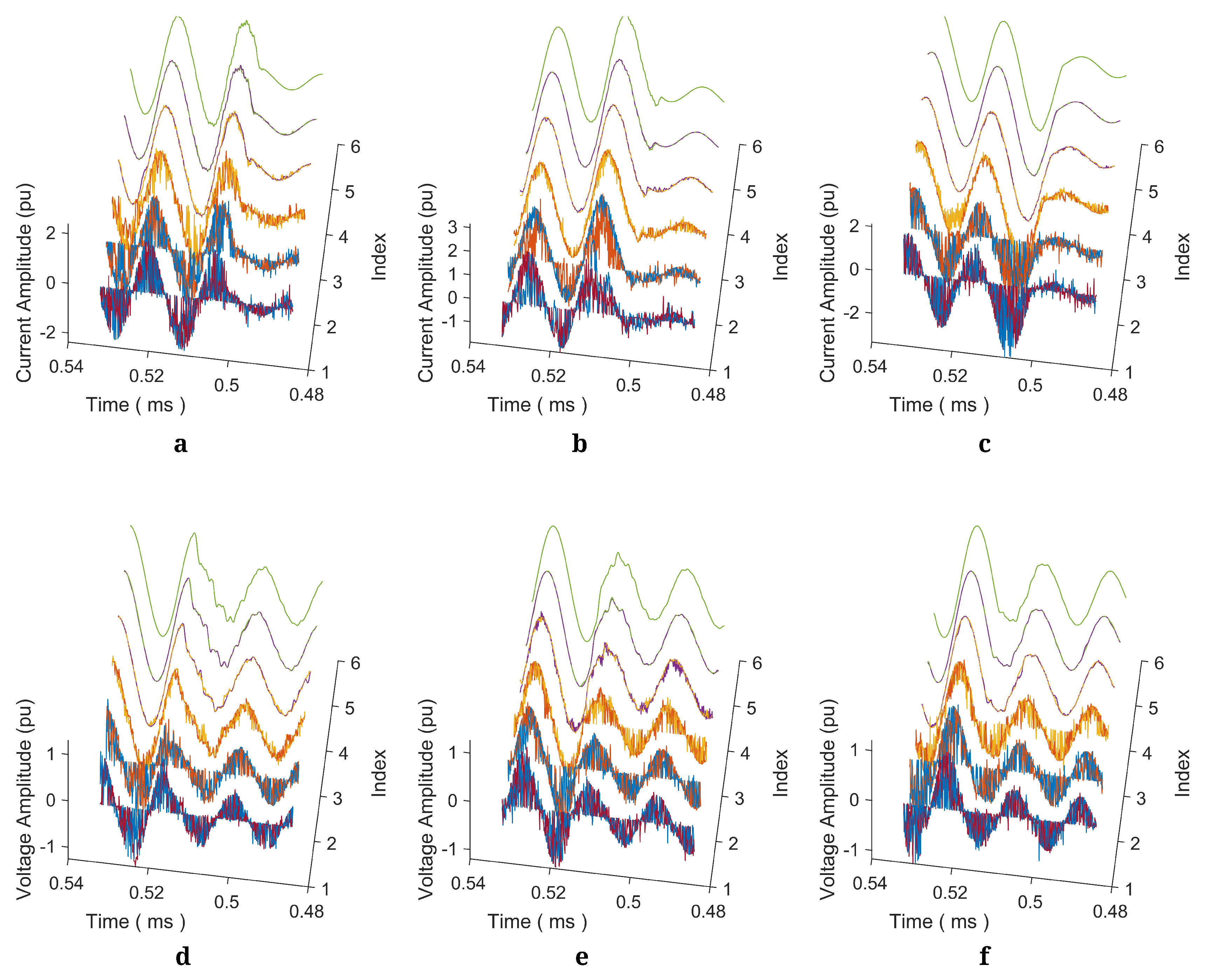
Figure 7 shows the reconstruction of the signal at a different point in the system based on 50% to 100% random samples; thus, the value of k will be 171. It is important to mention that the reconstructed signals were obtained from 80% of the whole information, where orange signals eliminate the noise that occurs when the samples are spread. The machine time to execute this algorithm in order to find the optimal value k was lower than 0.2 s.
4.2. Orthogonal Matching Pursuit Results
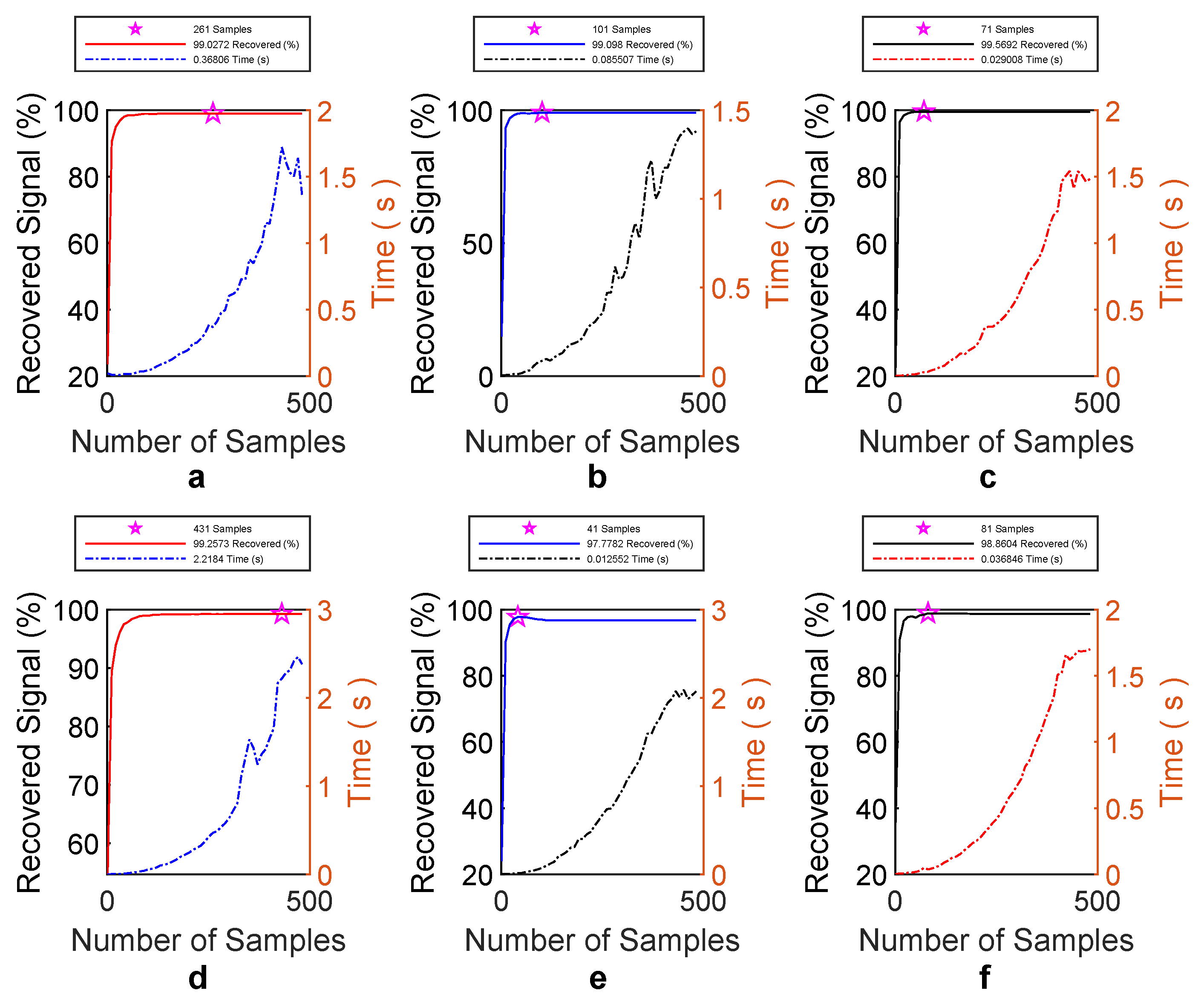
To solve the problem of signal restoration using the orthogonal matching pursuit model, it is necessary to establish the number of atoms of the signal known as k. The atoms of the signal are the samples of the signal that represent the entire signal. Figure 8 shows the optimal number k “atoms” of the fault signal. It is shown that the number of random samples needed by the atoms was 431 (Part d) for a signal under fault conditions without noise. The machine time of the algorithm was less than 1.71 s.
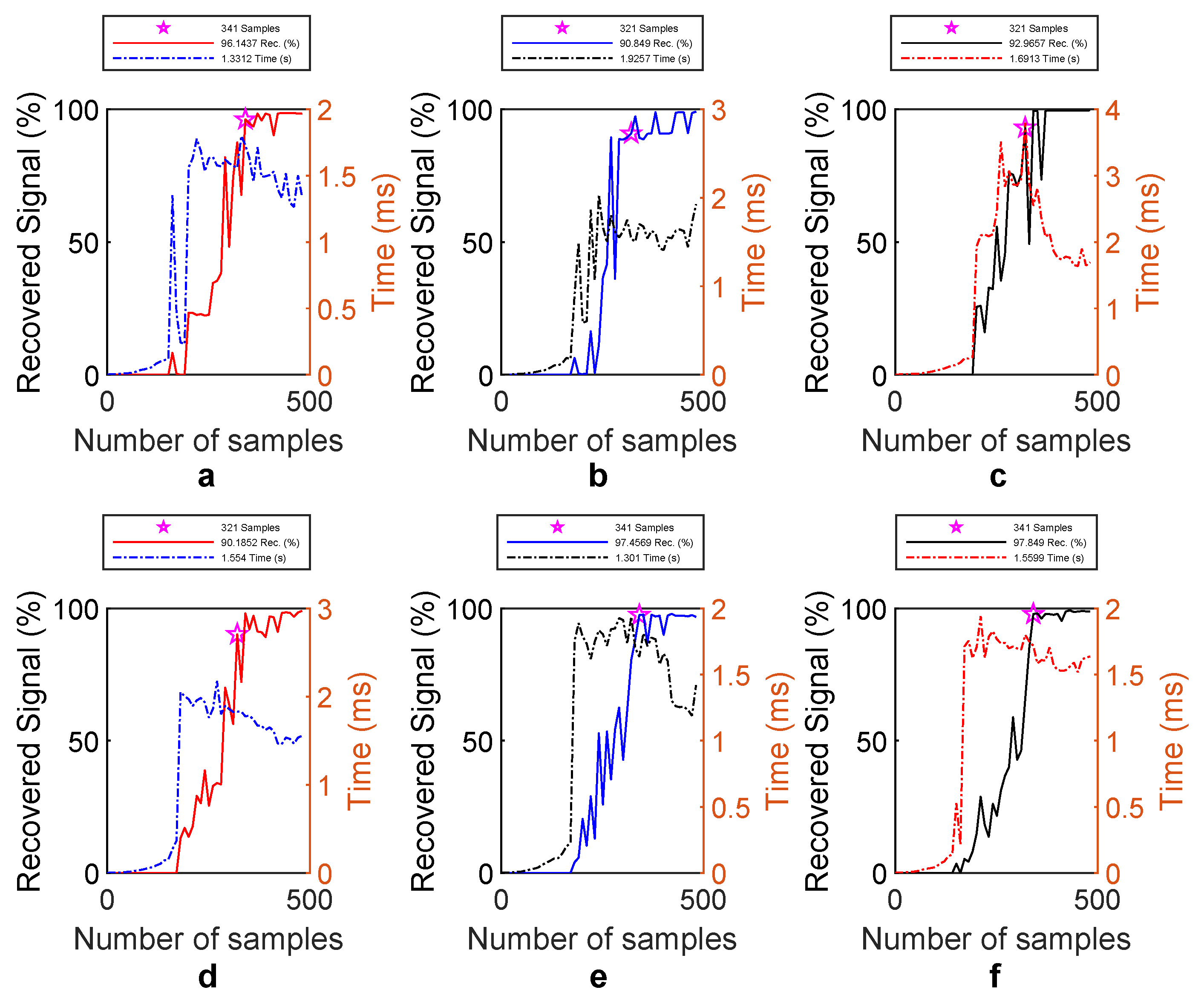
Figure 9 shows the number of samples needed to reconstruct 90% of the signal with respect to the original one. The scenario with the highest number required 341 random samples of the original signal (Parts a and e); however, Part e requires a lower time for the solution of the algorithm, which was 0.182 s.
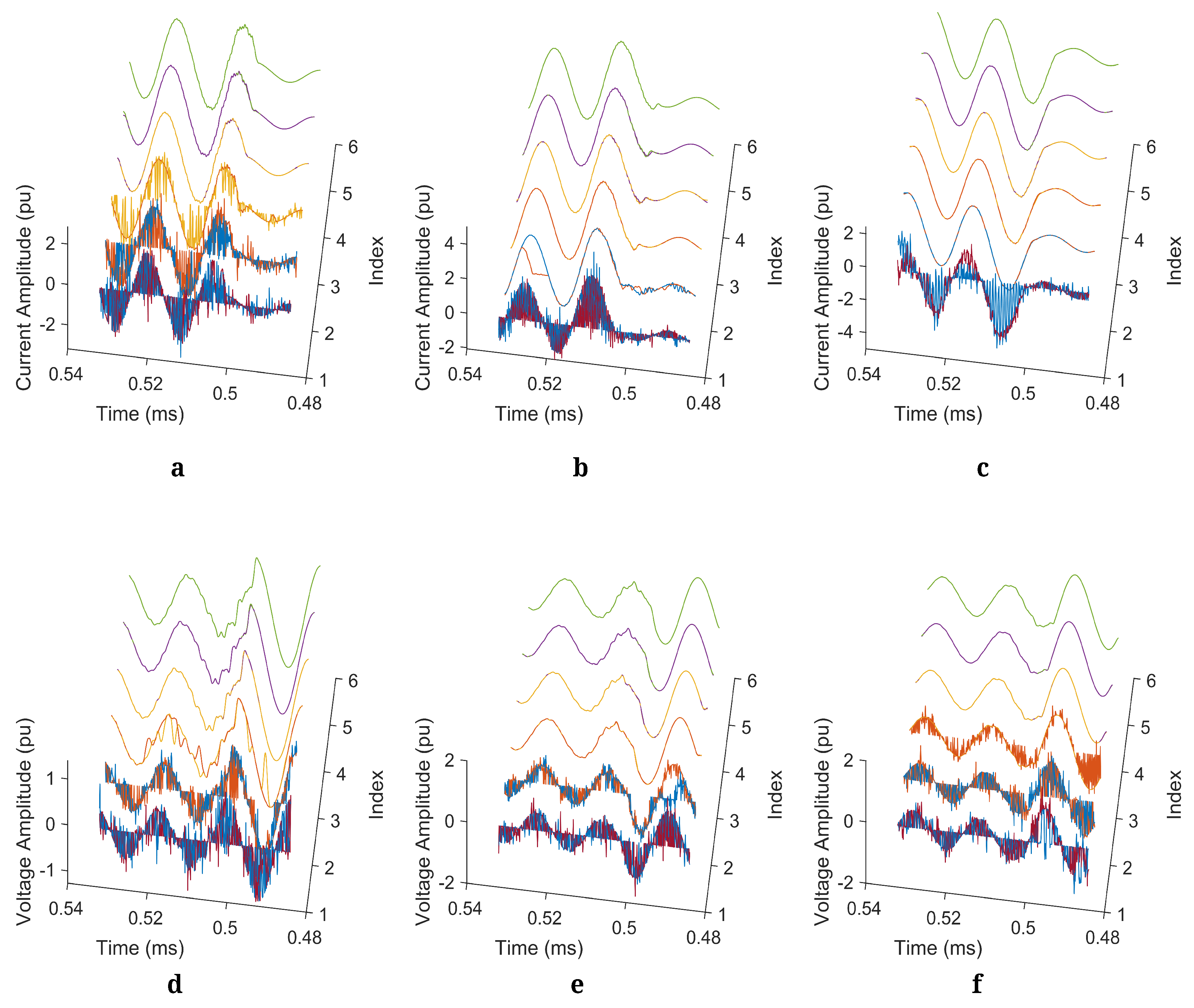
Figure 10 shows the reconstruction of the signal at a different point in the system based on 50% to 100% of random samples; thus, the value of k will be 431, as was described previously. It is important to mention that the reconstructed signals were obtained from 60% of the whole information, where orange signals eliminate the noise that occurs when the samples are spread.
4.3. Basis Pursuit Results
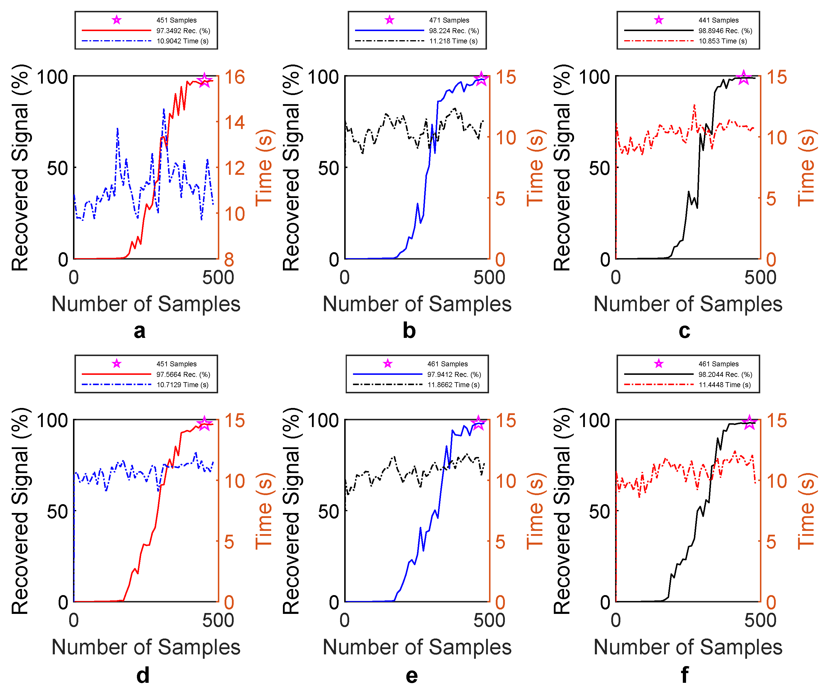
Figure 11 shows the number of samples needed to reconstruct 90% of the signal with respect to the original one. The scenario with the lowest number required 441 random samples of the original signal (Part c), and the time required for the solution of the algorithm was approximately 10.71 s, which was also the lowest time compared to the other samples analyzed in the other subfigures of the same figure.
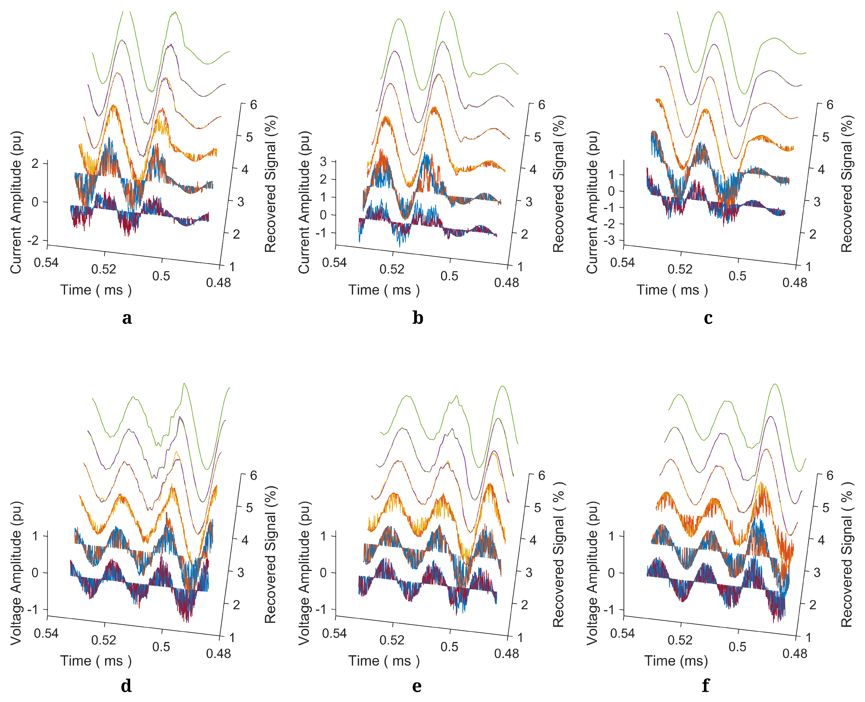
Figure 12 shows the reconstruction of the signal at a different point in the system based on 50% to 100% of random samples; thus, the value of k will be 431. It is important to mention that the reconstructed signals were obtained from 60% of the whole information, where orange signals eliminate the noise that occurs when the samples are spread.
The Table 1 presents the summary of the different BP, MP, and OMP techniques used for signal reconstruction based on compressed sensing. The number of k and m samples necessary to reconstruct the signals is described. The error percentage and the recovery time are detailed as well.
5. Conclusions
- The results obtained in the paper demonstrated that by determining the optimal points of the number of k atoms and the number of spread samples of the signal, between 60 and 80 percent of the original signal could be reconstructed, taking into account that with a smaller number of random samples, the higher the signal reconstruction time.
- It was demonstrated that real-time signal processing algorithms, such as matching pursuit, were a helpful tool that must be implemented due to their quick response in order to find the original signal based on spread signals obtained from sampling. Thus, this algorithm could reconstruct the signal with a random number of samples, approximately 171, greater than 80% of the original one, and the algorithm solution times were less than 0.2 s. This method offered the best of the three solutions because it reconstructed the original signal almost entirely in a short period.
- According to the results obtained, it was evident that the orthogonal matching pursuit solution allowed building a signal from a smaller amount of signals, 60% of the dispersed samples. The number of atoms obtained was 431, and the restoration time was almost 2 s, which was 10 times longer than matching pursuit. Consequently, this was not the best option due to the fact that with a higher number of samples, only a little more than half of the desired signal was obtained.
- It was also evident that the basis pursuit solution allowed building a signal from a smaller amount of spread signals, but its execution time was 100 times longer than matching pursuit because it took almost 12 s in order to reconstruct almost 70% of the signal. The higher the number of samples, the longer the restoration times. As a consequence, this method would not be the best option mainly because it had a high amount of machine time.
Author Contributions
Conceptualization, methodology, software, resources, validation, and formal analysis, M.R.; investigation, writing, original draft preparation, M.R. and I.M. All authors read and agreed to the published version of the manuscript.
Funding
This work was supported by Universidad Politécnica Salesiana and Grupo de Investigación en Redes Eléctricas Inteligentes–GIREI under the project Real-time electrical fault classification in transmission lines based on advanced signal processing techniques.
Conflicts of Interest
The authors declare no conflict of interest.
Abbreviations
| BP | Basis Pursuit |
| CS | Compressed Sensing Theory |
| DCT | Discrete Cosine Transform |
| DSP | Digital Signal Processing |
| GT | Gabor Transform |
| GWT | Gabor–Wigner Transform |
| HHT | Hilbert-–Haung Transform |
| HT | Hilbert Transform |
| LS | Least Squares |
| MP | Matching Pursuit |
| OMP | Orthogonal Matching Pursuit |
| PMU | Phasor Measurement Unit |
| PQ | Power Quality |
| PS | Power Systems |
| RIP | Restricted Isometric Property |
| SG | Smart Grid |
| SP | Signal Processing |
| ST | S-Transform |
| STFT | Short-Time Fourier Transform |
| WDF | Wigner Distribution Function |
| WT | Wavelet Transform |
References
- Vega, T.Y.; Roig, V.F.; San Segundo, H.B. Evolution of signal processing techniques in power quality. In Proceedings of the 2007 9th International Conference on Electrical Power Quality and Utilisation, EPQU, Barcelona, Spain, 9–11 October 2007. [Google Scholar] [CrossRef]
- Karimi-Ghartemani, M.; Bakshai, A.; Eren, S. New generation of signal processing techniques for power system applications. In Proceedings of the 2007 IEEE Canada Electrical Power Conference, EPC 2007, Montreal, QC, Canada, 25–26 October 2007; pp. 256–260. [Google Scholar] [CrossRef]
- Lambert-Torres, G.; Fonseca, E.F.; Coutinho, M.P.; Rossi, R. Intelligent alarm processing. In Proceedings of the 2006 International Conference on Power System Technology, POWERCON2006, Chongqing, China, 22–26 October 2006. [Google Scholar] [CrossRef]
- Shi, L.B.; Chang, N.C.; Lan, Z.; Zhao, D.P.; Zhou, H.F.; Tam, P.T.; Ni, Y.X.; Wu, F.F. Implementation of a power system dynamic security assessment and early warning system. In Proceedings of the 2007 IEEE Power Engineering Society General Meeting, PES, Tampa, FL, USA, 24–28 June 2007; pp. 1–6. [Google Scholar] [CrossRef]
- Abiyev, A.N. A new digital signal processing based approach for evaluation of reactive power and energy in power distribution systems. In Proceedings of the Innovations’07: 4th International Conference on Innovations in Information Technology, IIT, Dubai, UAE, 18–20 November 2007; pp. 426–430. [Google Scholar] [CrossRef]
- Al-Nujaimi, A.; Al-Muhanna, A.; Zerguine, A. Digital signal processing effect on power system overcurrent protection relay behavior and operation time. In Proceedings of the 2017 9th IEEE-GCC Conference and Exhibition, GCCCE 2017, Manama, Bahrain, 8–11 May 2017; pp. 1–5. [Google Scholar] [CrossRef]
- Ignatova, V.; Styczynski, Z.; Granjon, P.; Bacha, S. Statistical matrix representation of time-varying electrical signals. reconstruction and prediction applications. In Proceedings of the 2006 9th International Conference on Probabilistic Methods Applied to Power Systems, PMAPS, Stockholm, Sweden, 11–15 June 2006; pp. 1–6. [Google Scholar] [CrossRef]
- Franco-Tinoco, C.; Astro-Bohorquez, R.; Garcia-Mora, D. A Signal Reconstruction Technique for Power Delivery Analysis. In Proceedings of the 2019 IEEE 10th Latin American Symposium on Circuits and Systems, LASCAS 2019, Armenia, Colombia, 24–27 February 2019; pp. 209–212. [Google Scholar] [CrossRef]
- Zhang, Q.; Chen, Y.; Chen, Y.; Chi, L.; Wu, Y. A cognitive signals reconstruction algorithm based on compressed sensing. In Proceedings of the 2015 IEEE 5th Asia-Pacific Conference on Synthetic Aperture Radar, APSAR 2015, Singapore, 1–4 September 2015; pp. 724–727. [Google Scholar] [CrossRef]
- Yan, B.; Lijun, T.; Yunxing, G.; Yanwen, H. Load modeling based on power quality monitoring system applied compressed sensing. In Proceedings of the 2017 IEEE Transportation Electrification Conference and Expo, Asia-Pacific, ITEC Asia-Pacific 2017, Harbin, China, 7–10 August 2017. [Google Scholar] [CrossRef]
- Sun, H.; Ni, L. Compressed sensing data reconstruction using adaptive generalized orthogonal matching pursuit algorithm. In Proceedings of the 2013 3rd International Conference on Computer Science and Network Technology, ICCSNT 2013, Dalian, China, 12–13 October 2013; pp. 1102–1106. [Google Scholar] [CrossRef]
- Chrétien, S. An alternating ℓ1 approach to the compressed sensing problem. IEEE Signal Process. Lett. 2010, 17, 181–184. [Google Scholar] [CrossRef]
- Tropp, J.A.; Gilbert, A.C. Signal recovery from random measurements via orthogonal matching pursuit. IEEE Trans. Inf. Theory 2007, 53, 4655–4666. [Google Scholar] [CrossRef] [Green Version]
- Chen, K.; Li, Z.; Cheng, J.; Zhou, Z.; Lu, H. A variational Bayesian approach to remote sensing image change detection. Int. Geosci. Remote Sens. Symp. (IGARSS) 2009, 3, III-204–III-207. [Google Scholar] [CrossRef]
- Rozenberg, I.; Levron, Y. Applications of compressed sensing and sparse representations for state estimation in power systems. In Proceedings of the 2015 IEEE International Conference on Microwaves, Communications, Antennas and Electronic Systems, COMCAS 2015, Tel Aviv, Israel, 2–4 November 2015. [Google Scholar] [CrossRef]
- Guo, L.P.; Kok, C.W.; So, H.C.; Tam, W.S. Two-band signal reconstruction from periodic nonuniform samples. In Proceedings of the 2019 27th European Signal Processing Conference (EUSIPCO), A Coruna, Spain, 2–6 September 2019; pp. 1–5. [Google Scholar] [CrossRef]
- Kumar, S. Illustrated Compressed Sensing. Creative Commons Attribution 3.0 Unported License. Delhi, India. 2014, p. 1. Available online: http://indigits.com/assets/research/notes_compressed_sensing.pdf (accessed on 21 April 2020).
- Mo, Q.; Shen, Y. A remark on the restricted isometry property in orthogonal matching pursuit. IEEE Trans. Inf. Theory 2012, 58, 3654–3656. [Google Scholar] [CrossRef]
- Song, C.B.; Xia, S.T. Sparse signal recovery by ℓq minimization under restricted isometry property. IEEE Signal Process. Lett. 2014, 21, 1154–1158. [Google Scholar] [CrossRef] [Green Version]
- Sahoo, S.K.; Makur, A. Signal recovery from random measurements via extended orthogonal matching pursuit. IEEE Trans. Signal Process. 2015, 63, 2572–2581. [Google Scholar] [CrossRef]
- Candes, E.J.; Tao, T. Near-optimal signal recovery from random projections: Universal encoding strategies? IEEE Trans. Inf. Theory 2006, 52, 5406–5425. [Google Scholar] [CrossRef] [Green Version]
- Donoho, D.L. For most large underdetermined systems of linear equations the minimal ℓ1-norm solution is also the sparsest solution. Commun. Pure Appl. Math. 2006, 59, 797–829. [Google Scholar] [CrossRef]
- Narayanan, S.; Sahoo, S.K.; Makur, A. Greedy pursuits based gradual weighting strategy for weighted ℓ1-Minimization. In Proceedings of the 2018 IEEE International Conference on Acoustics, Speech and Signal Processing (ICASSP), Calgary, AB, Canada, 15–20 April 2018; pp. 4664–4668. [Google Scholar] [CrossRef]
- Narayanan, S.; Sahoo, S.K.; Makur, A. PT US CR. Signal Process. 2017. [Google Scholar] [CrossRef]
- Carta, D.; Pegoraro, P.A.; Sulis, S. Impact of Measurement Accuracy on Fault Detection Obtained with Compressive Sensing. In Proceedings of the 2018 IEEE 9th International Workshop on Applied Measurements for Power Systems (AMPS), Bologna, Italy, 26–28 September 2018; pp. 1–5. [Google Scholar] [CrossRef]
- Wang, J.; Kwon, S.; Li, P.; Shim, B. Recovery of sparse signals via generalized orthogonal matching pursuit: A new analysis. IEEE Trans. Signal Process. 2016, 64, 1076–1089. [Google Scholar] [CrossRef] [Green Version]
- Li, H.; Ma, Y.; Fu, Y. An improve d RIP-base d performance guarantee for sparse signal recovery via simultaneous orthogonal matching pursuit. Signal Process. 2018, 144, 29–35. [Google Scholar] [CrossRef]
- Narayanan, S.; Sahoo, S.K.; Makur, A. Greedy pursuits assisted basis pursuit for compressive sensing. In Proceedings of the 23rd European Signal Processing Conference, EUSIPCO 2015, Nice, France, 31 August–4 September 2015. [Google Scholar] [CrossRef]
- Zhao, J.; Gómez-Expósito, A.; Netto, M.; Mili, L.; Abur, A.; Terzija, V.; Kamwa, I.; Pal, B.; Singh, A.K.; Qi, J.; et al. Power System Dynamic State Estimation: Motivations, Definitions, Methodologies, and Future Work. IEEE Trans. Power Syst. 2019, 34, 3188–3198. [Google Scholar] [CrossRef]
- Odejide, O.O.; Akujuobi, C.M.; Annamalai, A.; Fudge, G. Joint design of channel-source coding for compressive sampling systems. In Proceedings of the 2010 7th IEEE Consumer Communications and Networking Conference, CCNC 2010, Las Vegas, NV, USA, 9–12 January 2010. [Google Scholar] [CrossRef]
- Zhang, Y.; Zhang, J.; Ma, J.; Wang, Z. Fault diagnosis based on BFS in electric power system. In Proceedings of the 2009 International Conference on Measuring Technology and Mechatronics Automation, ICMTMA 2009, Zhangjiajie, Hunan, China, 11–12 April 2009; Volume 1, pp. 643–646. [Google Scholar] [CrossRef]
- He, S.; Yang, D.; Li, W.; Xia, Y.; Tang, Y. Detection and fault diagnosis of power transmission line in infrared image. In Proceedings of the 2015 IEEE International Conference on Cyber Technology in Automation, Control and Intelligent Systems, IEEE-CYBER 2015, Shenyang, China, 8–12 June 2015; pp. 431–435. [Google Scholar] [CrossRef]
Figure 1.
Management and control of the electrical power system.

Figure 2.
Framework of compressed sensing [17].
Figure 2.
Framework of compressed sensing [17].

Figure 3.
Electrical fault in the power system IEEE 39-bar.

Figure 4.
(a) Time signals of current at bus 4, (b) frequency spectrum of current at bus 4, (c) DCT index of current at bus 4, (d) Time signals of voltage at bus 4, (e) frequency spectrum of voltage at bus 4, (f) DCT index of voltage at bus 4.
Figure 4.
(a) Time signals of current at bus 4, (b) frequency spectrum of current at bus 4, (c) DCT index of current at bus 4, (d) Time signals of voltage at bus 4, (e) frequency spectrum of voltage at bus 4, (f) DCT index of voltage at bus 4.

Figure 5.
Calculation of the number of k atoms vs. processing time ((a–c) current and (d–f) voltage at bus 4).
Figure 5.
Calculation of the number of k atoms vs. processing time ((a–c) current and (d–f) voltage at bus 4).

Figure 6.
Number of m samples necessary to recover the original signal vs. processing time ((a–c) current and (d–f) voltage at bus 4).
Figure 6.
Number of m samples necessary to recover the original signal vs. processing time ((a–c) current and (d–f) voltage at bus 4).

Figure 7.
Signal reconstruction using k and m values vs. processing time ((a–c) current and (d–f) voltage at bus 14).
Figure 7.
Signal reconstruction using k and m values vs. processing time ((a–c) current and (d–f) voltage at bus 14).

Figure 8.
Calculation of the number of k atoms vs. processing time ((a–c) current and (d–f) voltage at bus 4).
Figure 8.
Calculation of the number of k atoms vs. processing time ((a–c) current and (d–f) voltage at bus 4).

Figure 9.
Number of m samples needed to recover the signal vs processing time ((a–c) current and (d–f) voltage at bus 4).
Figure 9.
Number of m samples needed to recover the signal vs processing time ((a–c) current and (d–f) voltage at bus 4).

Figure 10.
Signal reconstruction using k and m values vs. processing time ((a–c) current and (d–f) voltage at bus 14).
Figure 10.
Signal reconstruction using k and m values vs. processing time ((a–c) current and (d–f) voltage at bus 14).

Figure 11.
Number of samples m needed to recover the signal vs. processing time ((a–c) current and (d–f) voltage at bus 4).
Figure 11.
Number of samples m needed to recover the signal vs. processing time ((a–c) current and (d–f) voltage at bus 4).

Figure 12.
Signal reconstruction using m values vs. processing time ((a–c) current and (d–f) voltage at bus 14).
Figure 12.
Signal reconstruction using m values vs. processing time ((a–c) current and (d–f) voltage at bus 14).


Table 1.
Results of signal reconstruction techniques.
| k Samples | BP (%) | MP (%) | OMP (%) |
| Current | N/A | 35.4 | 54.1 |
| Voltage | N/A | 35.4 | 89.2 |
| m Samples | BP (%) | MP (%) | OMP (%) |
| Current | 90.9 | 76.8 | 70.6 |
| Voltage | 93.4 | 80.9 | 70.6 |
| Error | BP (%) | MP (%) | OMP (%) |
| Current | 1.105 | 4.451 | 3.856 |
| Voltage | 2.433 | 4.784 | 2.151 |
| Time for Recovery | BP (s) | MP (s) | OMP (s) |
| Current | 10.853 | 0.182 | 1.331 |
| Voltage | 10.712 | 0.191 | 1.559 |
© 2020 by the authors. Licensee MDPI, Basel, Switzerland. This article is an open access article distributed under the terms and conditions of the Creative Commons Attribution (CC BY) license (http://creativecommons.org/licenses/by/4.0/).
Share and Cite
MDPI and ACS Style
Ruiz, M.; Montalvo, I. Electrical Faults Signals Restoring Based on Compressed Sensing Techniques. Energies 2020, 13, 2121. https://0-doi-org.brum.beds.ac.uk/10.3390/en13082121
AMA Style
Ruiz M, Montalvo I. Electrical Faults Signals Restoring Based on Compressed Sensing Techniques. Energies. 2020; 13(8):2121. https://0-doi-org.brum.beds.ac.uk/10.3390/en13082121
Chicago/Turabian StyleRuiz, Milton, and Iván Montalvo. 2020. "Electrical Faults Signals Restoring Based on Compressed Sensing Techniques" Energies 13, no. 8: 2121. https://0-doi-org.brum.beds.ac.uk/10.3390/en13082121
Note that from the first issue of 2016, this journal uses article numbers instead of page numbers. See further details here.