A Deep Recurrent Neural Network for Non-Intrusive Load Monitoring Based on Multi-Feature Input Space and Post-Processing

Abstract

Non-intrusive load monitoring (NILM) is a process of estimating operational states and power consumption of individual appliances, which if implemented in real-time, can provide actionable feedback in terms of energy usage and personalized recommendations to consumers. Intelligent disaggregation algorithms such as deep neural networks can fulfill this objective if they possess high estimation accuracy and lowest generalization error. In order to achieve these two goals, this paper presents a disaggregation algorithm based on a deep recurrent neural network using multi-feature input space and post-processing. First, the mutual information method was used to select electrical parameters that had the most influence on the power consumption of each target appliance. Second, selected steady-state parameters based multi-feature input space (MFS) was used to train the 4-layered bidirectional long short-term memory (LSTM) model for each target appliance. Finally, a post-processing technique was used at the disaggregation stage to eliminate irrelevant predicted sequences, enhancing the classification and estimation accuracy of the algorithm. A comprehensive evaluation was conducted on 1-Hz sampled UKDALE and ECO datasets in a noised scenario with seen and unseen test cases. Performance evaluation showed that the MFS-LSTM algorithm is computationally efficient, scalable, and possesses better estimation accuracy in a noised scenario, and generalized to unseen loads as compared to benchmark algorithms. Presented results proved that the proposed algorithm fulfills practical application requirements and can be deployed in real-time.

1. Introduction

Energy conservation in residential and commercial buildings through smart electrification has been a hot topic for researchers in recent years [1,2]. Because of the large deployments of smart meters, non-intrusive load monitoring (NILM) has become a very valuable tool to achieve this objective. NILM or simply energy disaggregation system estimates power consumption of individual household appliances or other electrical apparatus from an aggregated power signal, which is acquired through single-point sensing from a smart meter using some supervised/unsupervised technique [3,4]. A practical NILM system can provide real-time actionable feedback to consumers that gives them an idea about an individual appliance operation state, its power consumption, and cumulative energy usage. Studies have shown that appliance specific feedback urges the consumer to use energy wisely which as a result can save up to 12% energy in residential and commercial buildings [5,6]. For utility companies, this information can be useful in foreseeing the power demands, and efficiently operate electric power facilities [7].

The most efficient and cost-effective approach to achieve energy conservation goals through NILM is to use intelligent yet practically feasible algorithms. Existing disaggregation algorithms use either low or high frequency sampled electrical signatures to perform the NILM task [8]. However, being able to provide power consumption information for all types of appliances (type-1, type-2, type-3, and type-4) [9] is not adequate for practical application. There are some requirements such as scalability [10], performance in the presence of unidentified appliances, and generalization [11] that must be satisfied by the disaggregation algorithm to be used for the practical NILM system. Earlier NILM research was focused on identifying appliance states and their classification using signature-based [12,13,14,15,16] and event-based approaches [9,17,18]. However, these works were restricted to the identification and classification of type-1 appliances only due to their simple architecture. Additionally, transient-signature based approaches require a high sampling rate to capture transients, which is its major drawback for practical application [19].

In recent years, learning-based approaches are proposed to classify and directly estimate the power consumption of type-1 and type-2 appliances from an aggregated signal. Learning-based approaches are further classified into unsupervised [17] and supervised learning [20]. Unsupervised learning-based approaches do not require pre-training thus, they are more suitable for real-world application. Most recent works relevant to this category used the Hidden Markov Model (HMM) and its variants to disaggregate various types of appliances with reasonable classification accuracies [21,22,23]. A combination of Additive HMM (AFHMM) and Differential HMM (DFHMM) was proposed in [22] which was improved by [24] where inference on multiple HMMs set of states was computed using the Maximum a Posteriori (MAP) algorithm. Although FHMM-based NILM approaches are extensively used for power disaggregation, their performance is limited to the accurate approximation of appliance actual power consumption especially for type-2 (multi-state) and type-4 (always-on) appliances. Moreover, HMM-based methods have been reported to suffer from scalability and generalization, which limits its real-world application. Supervised learning based approaches used either machine learning (feed-forward neural networks [25], support vector machines [26]) or deep neural networks (DNN) to fulfil the NILM objective.

In contrast to classical event-based and state-based approaches, deep neural networks are capable of dealing with time complexity issues, scalability issues, and can learn very complex appliance signatures if trained with sufficient data [11,19]. Most recent NILM works employing deep neural networks used 1/6-Hz or 1/3-Hz sampled active power measurement as an input feature to train various deep neural networks such as long short-term memory (LSTM) networks [27,28,29,30], denoised autoencoder [31,32] and convolutional neural networks (CNN) [33,34,35,36]. Kelly [31] and He [29] proposed a LSTM based deep neural network architecture and trained it using 6-sec sampled data with only active power as an input feature. Their LSTM based DNN model was unable to identify multi-state appliances. To solve the multi-state appliance identification issue, Mauch and Yang [27] proposed a two-layer bidirectional LSTM based DNN model. They also evaluated their models on unseen test data to ensure the generalization capability. Similarly, Zhang et al. [35] proposed a two-step approach to identify multi-state appliances. They used a deep CNN model to identify the type of appliances and then used a k-means clustering algorithm to calculate the number of states of appliances. Zhang et al. [33] proposed sequence-to-point learning-based CNN architecture and evaluated it on 3-sec and 6-sec sampled data with only active power as an input feature. D’Incecco et al. [36] took one step further and evaluated Zhang’s [33] sequence-to-point algorithm performance on new unseen dataset to ensure transferability across appliances and datasets. However, their cross-domain transfer learning approach required fine-tuning of fully connected layers before performing load disaggregation that might cause a delay during online disaggregation if implemented in real-time.

In context, existing DNN-based disaggregation algorithms have shown better performance in terms of scalability and learning feature-rich appliance signatures. However, the practical feasibility of these approaches is still an open problem [11,37]. From an algorithm point-of-view, high power estimation accuracy and generalization are two most essential abilities that an algorithm should possess in order to be feasible for practical application. DNN models can be made generalized and highly accurate if they are trained on a large quantity of data and/or by performing hyperparameter optimization [31], [38]. Training machine learning or deep learning models on a huge amount of data with lots of features does not guarantee the best performance due to some misleading and irrelevant features [39]. However, low time complexity and better performance can be achieved with limited data if it is comprised of the most effective features [40,41]. Previous DNN-based works used either steady-state active power, reactive power or both as input features. Similarly, [42] showed that apart from active power, other electrical features (line current, line voltage, neutral current, and load angle) significantly improve the events classification accuracy for non-linear appliances. This implies that many electrical features, when combined to make a feature space can be a substitute for DNN models requiring a high amount of data for training. Recent multi-feature input based NILM approaches [24,43,44] selected the steady-state features using experiments and previous knowledge. Although those approaches reported an overall improvement in accuracy. However, disaggregation performance of individual loads deteriorated in some cases because of the ineffectiveness of selected feature(s) on individual appliances. Therefore, there is a need to determine a comprehensive set of features that can aid in disaggregating all types of appliances with high estimation accuracy and lowest generalization error. For that purpose, the influence of steady-state electrical features on the power consumption of individual appliances should be analyzed to make an intuition about relevant and most effective features.

At the disaggregation stage, deep neural networks tend to predict irrelevant activations, which does not belong to target appliance activations. Kong et al. [45] tackled this problem through post-processing, which included training a separate deep CNN model to classify predicted appliance activations. Their classification model ensured whether the predicted sequence belongs to a target appliance activation or not. Following a similar problem domain, this paper also proposes a training-less yet effective post-processing technique (as a part of disaggregation algorithm), which eliminates irrelevant activations by comparing the lengths of actual and predicted appliance activations.

In this paper, we explicitly focus on determining relevant and effective electrical features that can aid in achieving high estimation accuracy for type-1 and type-2 appliances, and generalized on unseen data. We present a multi-feature subspace for an LSTM (MFS-LSTM) algorithm that forms multi-feature input data by using the mutual information method and train deep LSTM models for individual appliances. The mutual information method measures the influence of steady-state electrical measurements on the active power consumption of individual appliances. From that information, relevant and most influential electrical features are selected to form multi-feature input data. This paper also proposes an effective post-processing technique that eliminates irrelevant appliance activations during the disaggregation stage and helps to keep predicted energy close to ground-truth energy. In addition, to make an effort towards a deployable deep learning-based NILM solution, we also design a three-stage practical NILM framework that intends to use pre-trained models (trained with the MFS-LSTM algorithm) to perform online disaggregation.

The rest of the paper is organized as follows. Section 2 introduces the MFS-LSTM algorithm in terms of multi-feature input space and post-processing. The design of a deep learning-based practical NILM framework is also discussed in Section 2. Section 3 presents a case study by providing details of the chosen dataset, model training, testing scenarios, and evaluation metrics. Section 4 presents the results. Section 5 concludes the work presented in this paper.

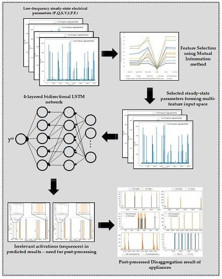
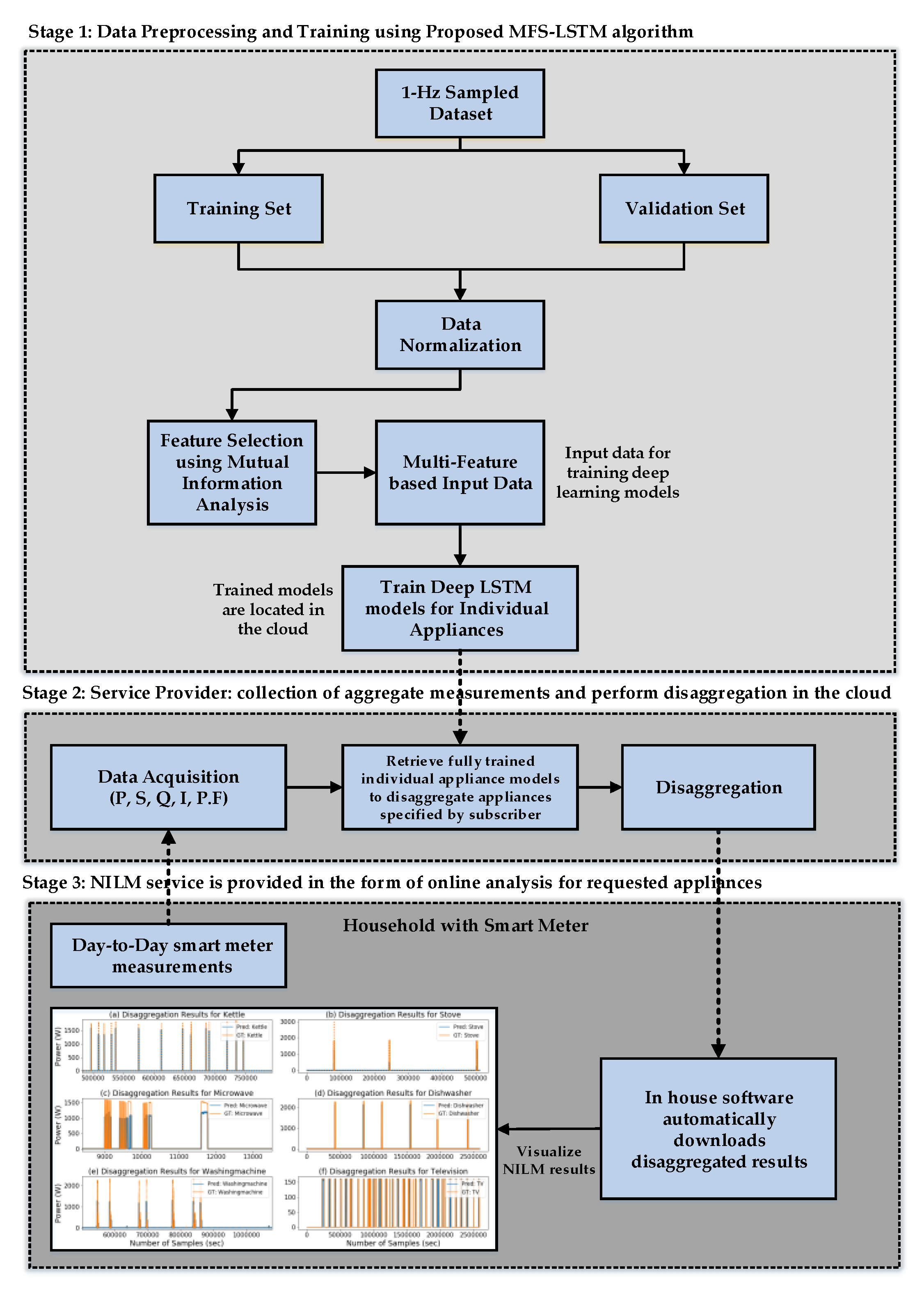
2. Proposed Energy Disaggregation Approach (MFS-LSTM Algorithm)

To achieve high estimation accuracy and lowest generalization error with a limited amount of data, this paper proposes a three-stage disaggregation algorithm based on a deep LSTM network. At the data pre-processing stage (first stage), multi-feature input data based on low-frequency electrical measurements were prepared that aims to extract more useful information from the limited training data. To prepare multi-feature input data; first, a mutual information principle was used to select the relevant and most effective features. A set of five features were used to make multi-feature input data for a deep LSTM network.

At the training stage (second stage), multi-feature input data were used to train four-layered bidirectional LSTM models for each target appliance. Hyperparameter optimization was performed to tune parameters that lead to the lowest training error and lowest convergence time for each deep LSTM model. At the third stage (disaggregation stage), a post-processing technique was employed to eliminate irrelevant appliance activations to improve disaggregation performance. Figure 1 shows the detailed architecture of our proposed energy disaggregation algorithm. Shaded regions in a grey color points-out the three stages of the disaggregation algorithm.

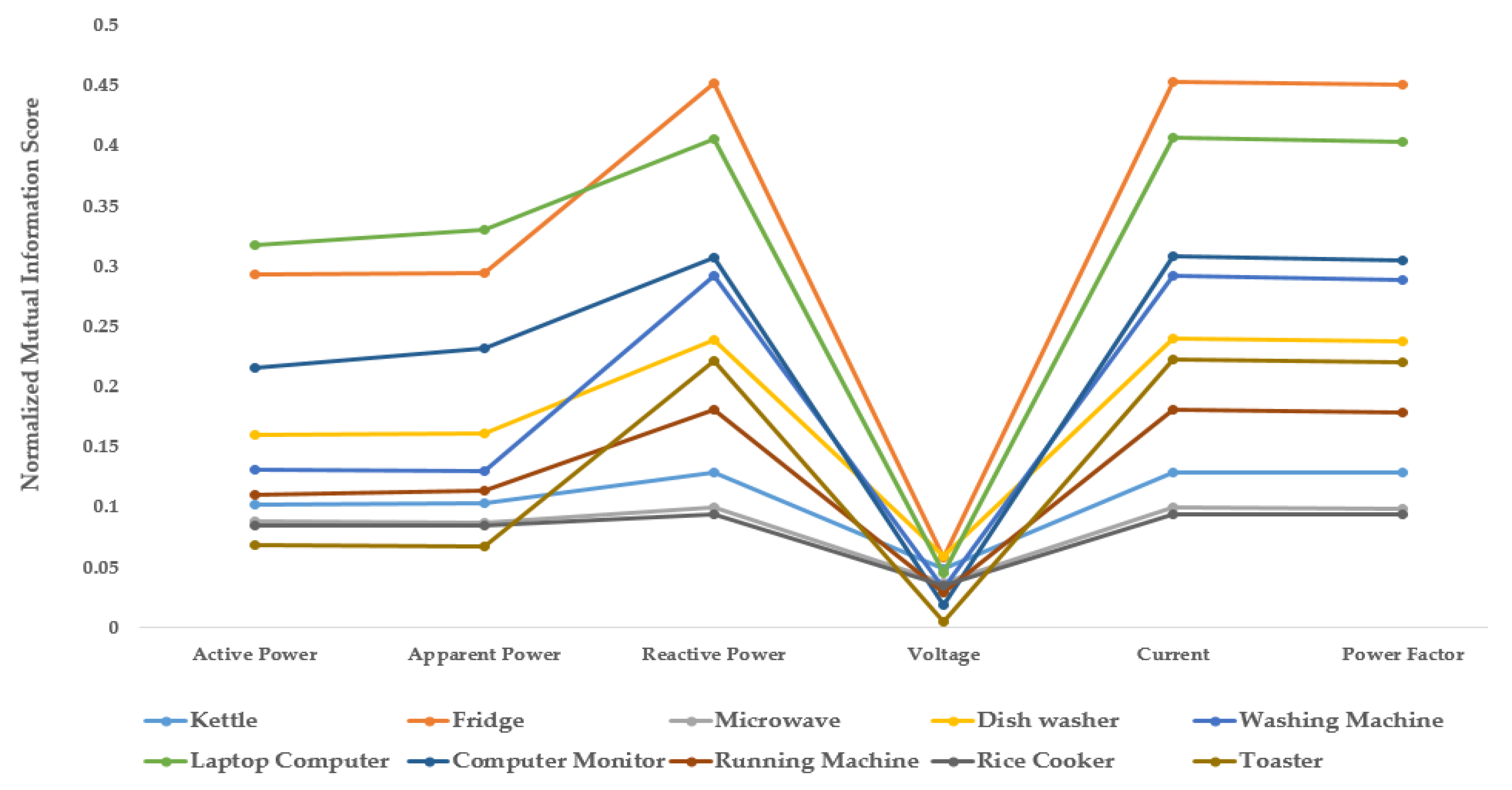
2.1. Steady-State Signatures as Multi-Feature Input Subspace

Input space construction is the starting point of any machine learning/deep learning modeling. In this paper, multi-feature input space was used to extract more information from the limited amount of data to improve the accuracy of the proposed deep recurrent neural networks (RNN)-based LSTM model.

In the field of NILM, variables including active power (P), apparent power (S), reactive power (Q), voltage ($V_{rms}$), current ($I_{rms}$), and power factor ($\cos \theta$) are available through measurement instruments and they are constrained by the following relationships:

$$\begin{array}{c}P=V_{rms}{I}_{rms}\cos \theta \\ Q=V_{rms}{I}_{rms}\sin \theta \\ S=\sqrt{P^2+Q^2}\end{array}$$

(1)

Equation (1) shows that all the variables provide some information that indicates an appliance’s state of operation and amount of power consumption. This implies that many electrical features, when combined to make a feature space, have so much to offer for energy disaggregation.

It would also be meaningful if we can analyze the influence of each electrical feature on the active power consumption of different type-1 and type-2 appliances so that insight into relevant and irrelevant features can be gained. For this purpose, he mutual information method is used in this paper. Mutual information measures share information contained in two variables, and knowing how much the value of one variable reduces the unpredictability on the other [46].

Previously in NILM research, the mutual information method is used for selecting delay parameters for different datasets [47] and for formulating utility-privacy trade-offs [48]. We have used the mutual information method to select relevant and most effective electrical features, which would make a feature space for our deep RNN model. First, the mutual information value between each electrical feature and power consumption of each target appliance was calculated using the formula stated in (2).

$$I\left(X, Y\right)={{\displaystyle \iint }}^{}p\left(x,y\right) \log \frac{p\left(x,y\right)}{p\left(x\right)p\left(y\right)}dxdy$$

(2)

where $p\left(x\right)$ and $p\left(y\right)$ are probability density functions of $x$ and $y$, and $p\left(x,y\right)$ denotes joint probability functions of two variables.

Secondly, results from (2) were combined in a tabular form, where rows represented power consumption of target appliances and columns represented each electrical feature considered for the analysis. Mutual information values were categorized into three ranges of strong, moderate, and weak influence. Those features, which had a weak influence on the power consumption of each target appliance were discarded, and those which had strong or moderate influence were selected to form multi-feature input space. This was unlike previous multi-feature NILM algorithms that made conclusions about relevant features based on the final results. Details of the mutual information analysis are provided in Section 3.1.

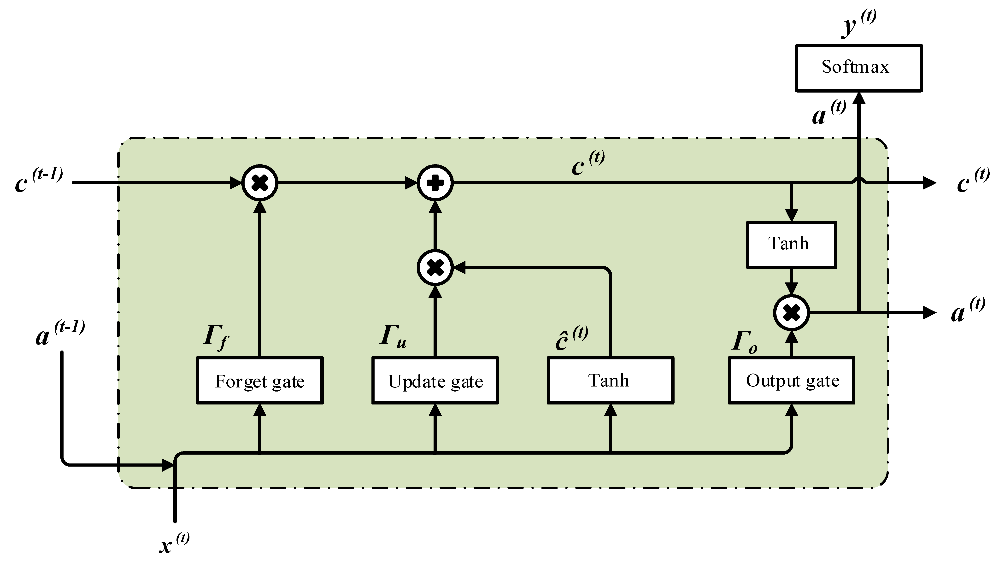
2.2. LSTM-based Deep Recurrent Neural Network

Deep recurrent neural networks (RNNs) are a variation of feed-forward neural networks that are used to process sequential data. Among the family of RNNs, the bidirectional LSTM network uses both previous and future information to predict current value; therefore, they are a natural fit for the NILM problem. In addition, they have longer memory and are able to deal with vanishing gradient problems [27,28].

Figure 2 shows the LSTM architecture in a single RNN unit. The decision on which information should be stored and which should be discarded is made by the forget layer (forget gate). The output of the forget gate is calculated using the weight and bias values of the current input sample x^(t) and information from the previous time step a^(t-1). This is represented by the following equation:

$${\Gamma }_f=\sigma \left(W_f\left[a^{\left(t-1\right)},x^{\left(t\right)}\right]+b_f\right)$$

(3)

where, ${\Gamma }_f$ is the output of the forget layer, $\sigma$ is the sigmoid function, $W_f$ is the weight for the forget layer, and $b_f$ is the bias value for the forget layer. The output of the forget layer can be either 0 or 1. Zero (0) means totally discard the information, and ‘1’ means totally store the information. Applying sigmoid activation to these values gives us the value of the forget state between 0 and 1. After discarding some information from the input sequence, a decision is made on what new information is to be stored at the current time step. This step is completed in two stages through the update gate and the Tanh layer (Tanh gate). The update gate works in the same manner as the forget gate and it decides which values will be updated using the following relationship:

$${\Gamma }_u=\sigma \left(W_u\left[a^{\left(t-1\right)},x^{\left(t\right)}\right]+b_u\right)$$

(4)

The Tanh layer creates a vector of new candidate values that could be added to the state. The ‘Tanh’ function is used in this step instead of the sigmoid function as shown in (5).

$${\widehat{c}}^{\left(t\right)}=\tan \mathrm{h}\left(W_c\left[a^{\left(t-1\right)},x^{\left(t\right)}\right]+b_c\right)$$

(5)

where, ${\widehat{c}}^{\left(t\right)}$ is the output of Tanh layer, $W_c$ is the weight for the Tanh layer, and $b_c$ is the bias value for the Tanh layer. The memory cell is updated from $c^{\left(t-1\right)}$ to $c^{\left(t\right)}$ in the third step. The new cell state $c^{\left(t\right)}$ is calculated using the information from the update gate (${\Gamma }_u$) and forget gate (${\Gamma }_f$) and the previous cell state ($c^{\left(t-1\right)}$):

$$c^{\left(t\right)}={\Gamma }_u\times {\widehat{c}}^{\left(t\right)}+{\Gamma }_f\times c^{\left(t-1\right)}$$

(6)

Th elast step is to update the activation function $a^{\left(t\right)}$ which is updated by multiplying the output gate with the current cell state.

$${\Gamma }_o=\sigma \left(W_o\left[a^{\left(t-1\right)},x^{\left(t\right)}\right]+b_o\right)$$

(7)

$$a^{\left(t\right)}={\Gamma }_o\times \tan \mathrm{h}\left(c^{\left(t\right)}\right)$$

(8)

Equations (4) to (8) are used to update the cell state of the LSTM in a single hidden unit. A deep LSTM architecture is a variation of LSTM where more than one LSTM hidden layers are stacked after each other to form a deep recurrent neural network.

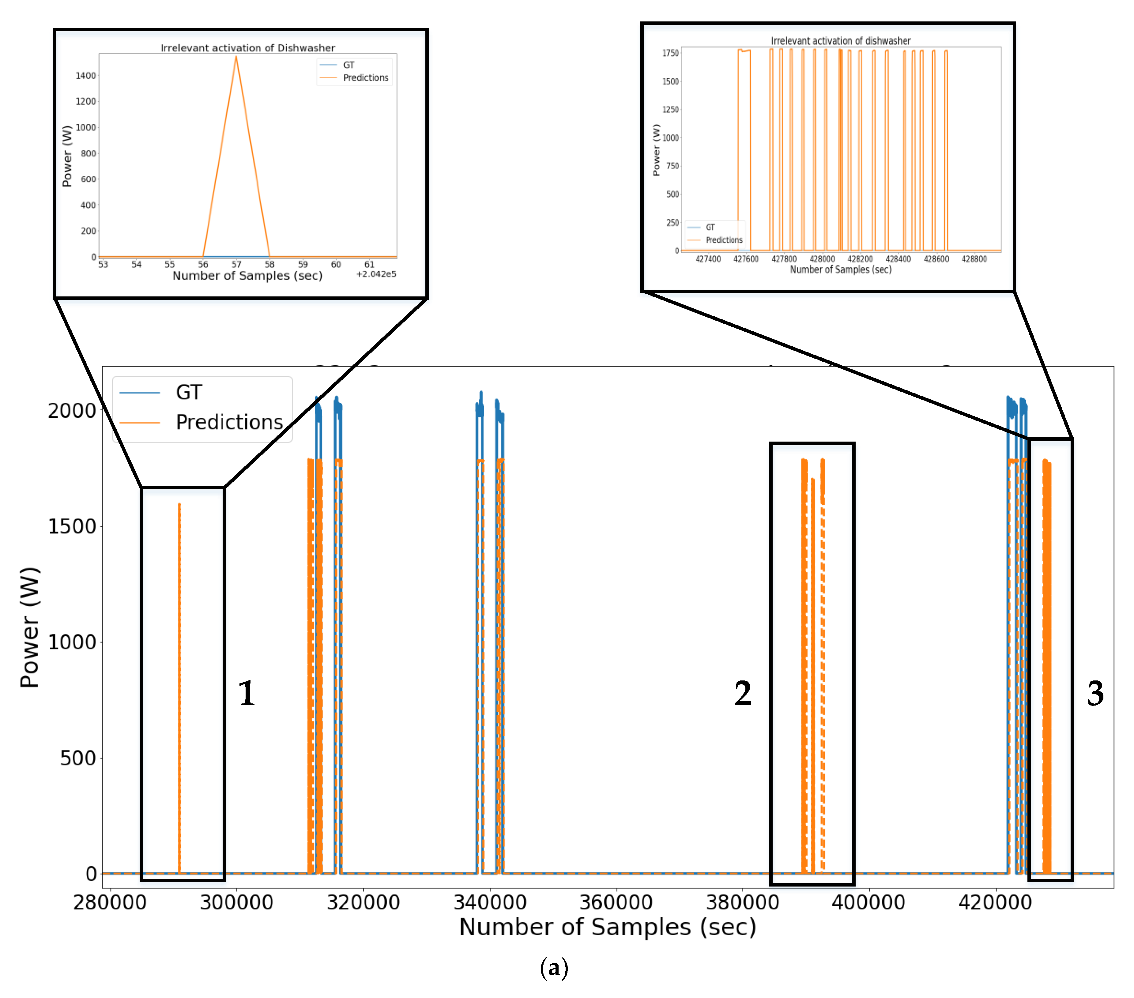
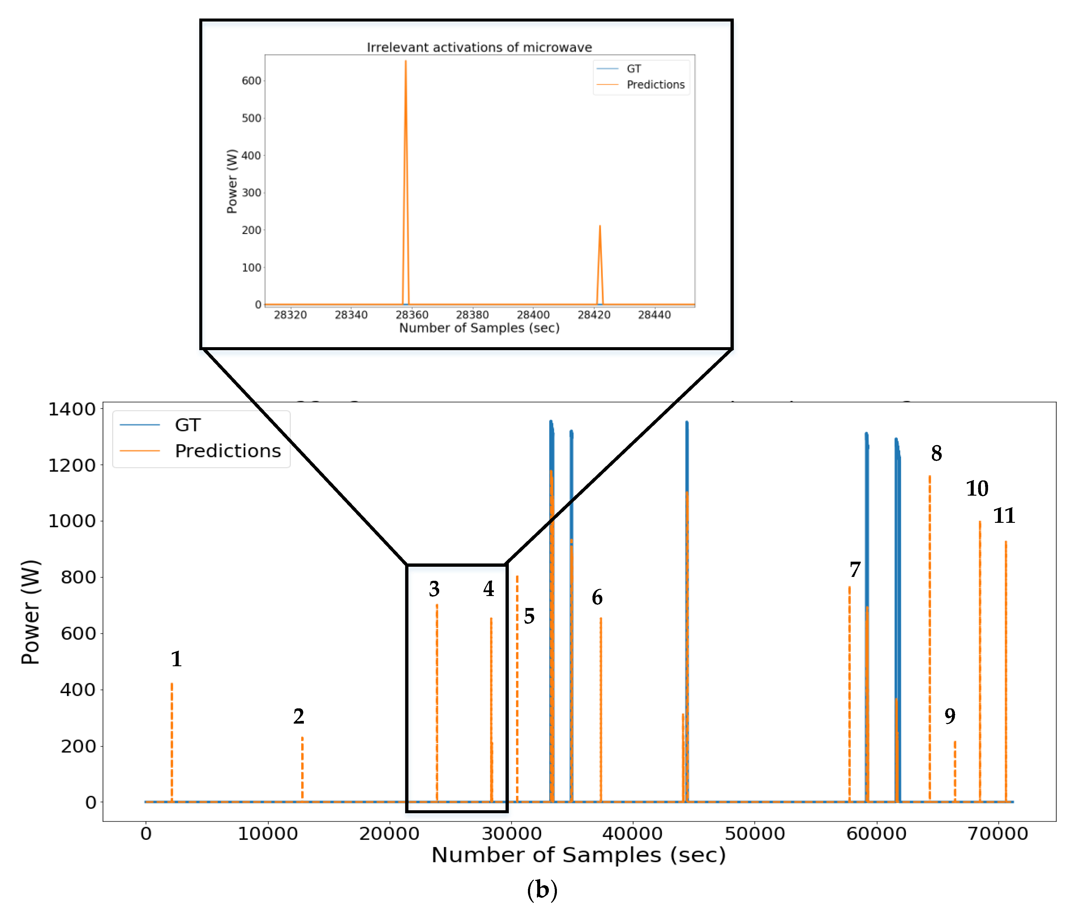
2.3. Post-Processing

Most of the type-1 and type-2 appliances have activation durations lasting from a few minutes (in the case of a microwave) to hours (dishwashers, washing machines) depending upon their actions to perform a task. However, predicted energy of target appliances not only contains ground-truth activations but some irrelevant activations as well, whose lengths (activation durations) are less than ground-truth activations as shown in Figure 3. These irrelevant activations lead to high false-positive cases that compromise the performance of the DNN algorithm.

Based on a visual analysis of irregular activations, an effective and robust post-processing technique is adopted in this paper. Unlike in [45], our proposed technique does not require training a separate DNN model. In fact, it eliminates irrelevant activations during the disaggregation stage by comparing the lengths of ground-truth and predicted appliance activations of both type-1 and type-2 appliances.

Our proposed post-processing algorithm is mainly composed of five steps. Given the ground-truth energy ($E_g$) and predicted energy profile ($E_p$), the first step is to calculate target appliance ground-truth activations $A_g=\left\{a_{1a}, a_{2a}, \cdots , a_{na}\right\}$ and predicted appliance activations $A_p=\left\{a_{1p}, a_{2p}, \cdots , a_{np}\right\}$. For that purpose, we use customized get_activations() function from NILMTK toolkit [49]. Here, ground-truth energy ($E_g$) refers to actual sub-metered power consumption of an appliance containing both ON and OFF events in a given period, and predicted energy ($E_p$) refers to estimated power consumption of an appliance by the algorithm.

At the second step, our post-processing algorithm calculates the length of ground-truth activations of a target appliance and creates a separate list of these activation lengths. The third step determines the minimum length from the list of ground-truth activations. At the fourth step, our post-processing algorithm compares minimum length with the length of every predicted appliance activation. At the fifth step, our algorithm eliminates all those predicted appliance activations whose length was less than the minimum length of ground-truth activations. In this way, we ensured that the total predicted energy is close to the ground-truth energy (sub-metered energy) of a target appliance. Details of the post-processing algorithm are provided in

Table 1. Detailed Post-Processing Algorithm.

Algorithm 1: Post-processing to eliminate irrelevant activations
1	Inputs: target appliance ground-truth activations set $A_g$ and predicted activations set $A_p$
2	Zero initialization of updated predicted activation profile (${\widehat{A}}_p$), and updated predicted energy profile (${\widehat{E}}_p$)
3	Calculate lengths of each activation from $A_g$ and $A_p$: $l_g=len\left\{A_g\right\}$ and $l_p=len\left\{A_p\right\}$
4	Determine minimum length from list of actual activations lengths: min{$l_g$}
5	Set pointer j = 0
6	For$jϵ\left(0,n\right):$
7	If $len\left(a_{jp}\right)<\min \left\{l_g\right\}$:
8	$a_{jp}=0$;
9	Update ${\widehat{A}}_p$ and ${\widehat{E}}_p$;
10	End if
11	End For
12	Return${\widehat{E}}_p$

.

2.4. Real-time Deployable NILM Framework

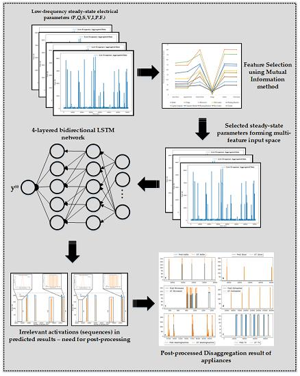
Existing deep learning-based NILM algorithms have used low-frequency steady-state measurements to disaggregate household appliances. However, those algorithms do not comply with practical application requirements such as generalization, the high number of disaggregated appliances, and high power estimation accuracy on a noised scenario. Therefore, those algorithms are not feasible for real-time deployment. As in this paper, we are proposing a multi-feature input space and post-processing based deep learning algorithm to achieve high estimation accuracy in a noised scenario and lowest generalization error on unseen data. Therefore, we attempted to design a real-time deployable NILM framework that incorporates our proposed MFS-LSTM algorithm.

Our proposed real-time deployable NILM framework intends to use pre-trained deep learning models (trained by the MFS-LSTM algorithm) to perform online disaggregation. Figure 4 shows the design of our three-stage deep learning-based practical NILM framework. At the first stage, deep LSTM models for individual appliances will be trained using the MFS-LSTM algorithm and will be integrated into the cloud-based server. This stage is called the data preprocessing and training stage because it prepares multi-feature input data and trains deep LSTM models according to the MFS-LSTM algorithm shown in Figure 1. In the second stage, the NILM service provider will collect the customer’s aggregate measurement (in the form of active power, apparent power, reactive power, current, and power factor) using a Consumer Access Device (CAD) [50] and will upload to the cloud server where online disaggregation will be performed using pre-trained deep LSTM models. The third stage refers to the NILM analysis in which post-processed disaggregation results along with energy consumption analysis will be downloaded to the customer.

3. Case Study

3.1. Datasets and Pre-Processing

Two publicly available datasets: UK-Domestic Appliance-Level Electricity (UK-DALE) dataset [50] and Electricity Consumption and Occupancy (ECO) dataset [51] were used for training and testing of our proposed algorithm. In UKDALE, aggregated mains power data is comprised of active power, apparent power, and voltage measurements; whereas sub-metered data contains only active power measurement sampled at 1/6 Hz, which we up-sampled to 1-Hz. The ECO dataset contains five electrical measurements, which are sampled at 1-Hz. Whereas, sub-meter data contains only active power measurements sampled at 1-Hz.

Based on the methodology given in Section 2.1, we considered six steady-state electrical measurements (active power, apparent power, reactive power, line voltage, line current, and power factor) for mutual information analysis, and the results are shown in Figure 5. As the mutual information score ranges between [0, +∞], we normalized it to lie in the range [0, 1]. Mutual information scores were categorized into three ranges: scores above 0.2 were considered high; scores between 0.1 and 0.2 were considered moderate, and; scores below 0.1 were considered weak.

There could be a couple of interpretations of these scores. The first noticeable factor was that reactive power, current, and power factors have higher scores as compared to other electrical features. This implies that these three electrical features have a high influence on all appliances’ power consumption except the kettle, microwave, and rice cooker. Similarly, active power and apparent power comparatively have less influence on all appliances with the score range between 0.103 and 0.318. Voltage is the only feature that had the weakest influence on all appliances. Therefore, we considered voltage as an irrelevant feature and selected only five electrical features to form the multi-feature input space for training the deep LSTM network. Another useful insight is that all electrical features (except voltage) have shown influence on all target appliances, which indicate that if these features are combined to form a multi-feature input space, then better disaggregation accuracy can be expected for all disaggregated appliances as compared to one or two feature-based input data.

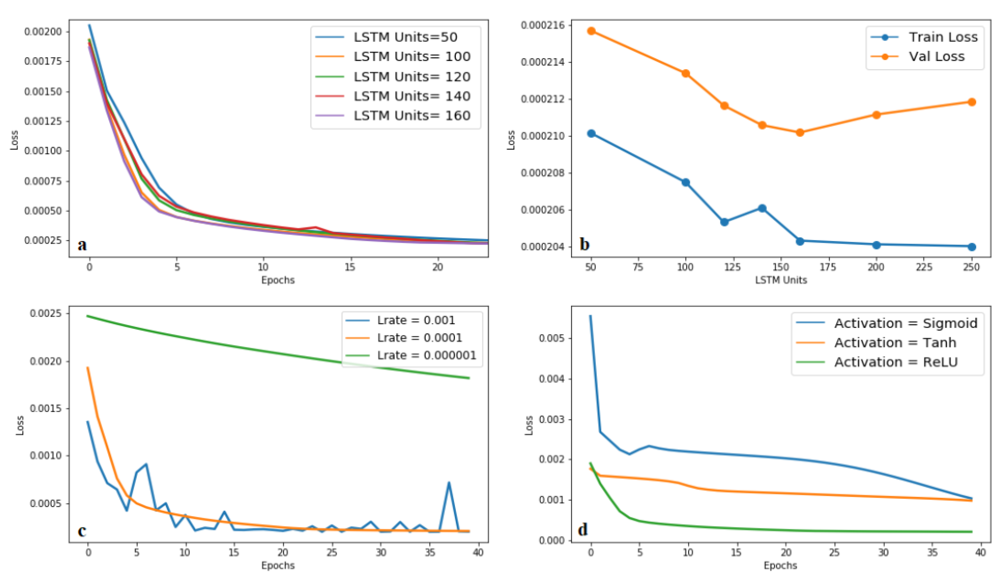
3.2. Training and Hyperparameter Optimization

For training deep LSTM (MFS-LSTM) models, at first, we split the input data into training data, validation data, and testing data. After data pre-processing, we trained our proposed architecture on multi-feature based training data using the Keras library [52] with GPU based Tensorflow as a backend engine. GPU used for training was NVIDIA GeForce GTX 1060 6GB.

We selected the LSTM architecture presented in [28] as our baseline model, which was composed of two hidden layers. We performed comprehensive hyperparameter tuning to select those hyperparameters values, which had the most influence on the learning behavior of the deep LSTM network for the reduction in the generalization error and convergence time. In particular, we focused mainly on three parameters: the number of hidden units, learning rate, and the activation function to see which combination of values aids in achieving local minima. We trained one model for each target appliance with different layer widths ranging from 50 to 250 for the first hidden layer. Whereas, the number of hidden units in the second layer was twice that of the first layer. We kept the number of units consistent with the first and second layers in each trial. This means the number of units in the second hidden layer varied from 100 to 500 (double of first layer units). Similarly, we varied the learning rate by the factor of 10 starting from 0.1 to 1 × 10⁻⁶. We also tried three activation functions depending upon the learning curve responses.

Figure 6a shows the learning behavior with varying layer widths corresponding to the first layer. Because, the number of units in each layer was varied simultaneously, the learning response shown in Figure 6a also stands for the second layer width. Increasing the layer width from 50 to 200 units demonstrated a downward response. Figure 6b shows the influence of the layer width on the training and validation loss. Increasing the hidden units (layer width) decreases the training loss but the network tends to overfit for larger units. This response urged us to use a layer width of 150 units for the first layer and 300 units for the second layer. Figure 6c shows the influence of the learning rate on the training loss. At a high learning rate, for instance, at 0.1, 0.001, the training loss and validation loss fluctuated, which revealed that the weights diverged, and the network was broken as a result. We ramped down the learning rate by a factor of 10 and achieved an optimal learning response at a learning rate of 1 × 10⁻⁴. Figure 6(d) shows the impact of the activation function on learning behavior. The rectified linear unit (ReLU) activation function was found to be the optimal activation function in our case. The dropout rate varied between 0.2 and 0.5 and a 0.3 rate was found to be the best in reducing overfitting.

After tweaking various hyperparameters, the four-layered deep recurrent neural network (deep LSTM) architecture was finalized. Complete architecture with optimized hyperparameter values are given below:

• 1D convolutional layer: input shape (5, 1), filter size = 4, and number of filters = 16
• 1 bidirectional LSTM layer: number of hidden units = 150, activation = ‘ReLu’
• Dropout layer with dropout = 0.3
• 1 bidirectional LSTM layer: number of hidden units = 300, activation = ‘ReLu’
• Dropout layer with dropout = 0.3
• Fully connected dense layer: number of units = 1, activation = ‘linear’

3.3. Performance Evaluation Metrics

In this paper, we have evaluated our approach considering the noised test data from house-2 and house-5 of the UKDALE dataset, and house-1 and house-2 of the ECO dataset. Percent noise ratio [37,38] was calculated on actual data using the following equation:

$$\%-NR=\frac{{{\displaystyle \sum }}_{t=1}^T\left|y_t-{{\displaystyle \sum }}_{k=1}^K{y}_t^k\right|}{{{\displaystyle \sum }}_{t=1}^T{y}_t}$$

(9)

Since our approach is based on classification and power estimation of target appliances, which requires both classification and estimation evaluation metrics to be used. We used state-based precision, recall, and F1 measure metrics, which are defined as:

$$precision=\frac{TP}{TP+FP}$$

(10)

$$recall=\frac{TP}{TP+FN}$$

(11)

$$F1=2\times \frac{precision\times recall}{precision+recall}$$

(12)

where TP, FP, and FN refer to the total number of true positives, false positives, and false negatives in the data, respectively. For power estimation evaluation, we have used the mean absolute error (MAE), signal aggregate error (SAE), and estimation accuracy (EA) metrics, which are defined in (13), (14), and (15), respectively:

$$MAE=\frac{1}{T}{\displaystyle \sum }_{t=1}^T\left|y_t-{\widehat{y}}_t\right|$$

(13)

where ${\widehat{y}}_t$ refers to predicted power at time t, and $y_t$ refers to ground truth power at time t.

$$SAE=\frac{\left|E_p-E_g\right|}{E_g}$$

(14)

where $E_p$ is total predicted energy and $E_g$ is total ground truth energy for each appliance. The estimation accuracy (EA) [53] metric was proposed to calculate the correct value of accuracy and error for power estimation based NILM problems. For each appliance, the estimation accuracy is defined as:

$$E{A}^k=1-\frac{{{\displaystyle \sum }}_{t=1}^T\left|{\widehat{y}}_t^k-y_t^k\right|}{2\times {{\displaystyle \sum }}_{t=1}^T{y}_t^k}$$

(15)

where ${\widehat{y}}_t^k$ is predicted power for appliance k at time t, and $y_t^k$ is ground truth power for appliance k at time t. K refers to the total number of target appliances and T refers to the total time sequence used for testing.

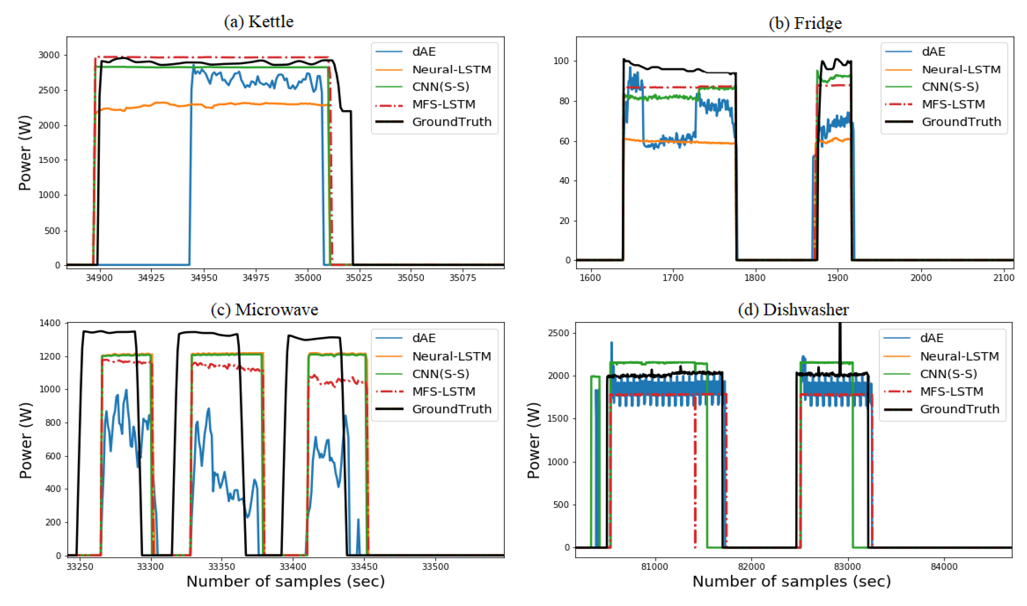
4. Results and Discussion

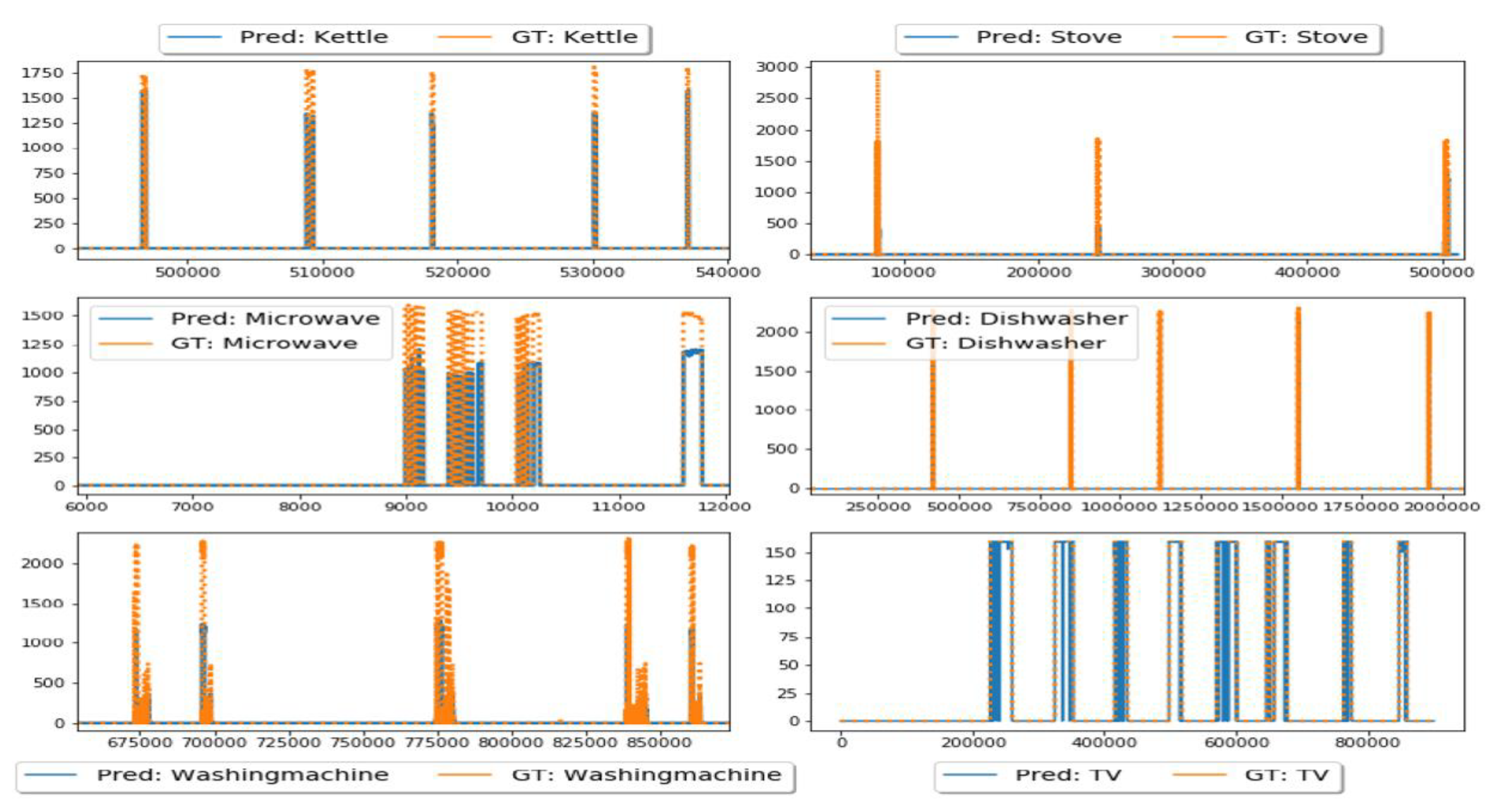
4.1. Testing in Seen Scenario (Unseen Data from UKDALE House-2 and ECO House-1,2,5)

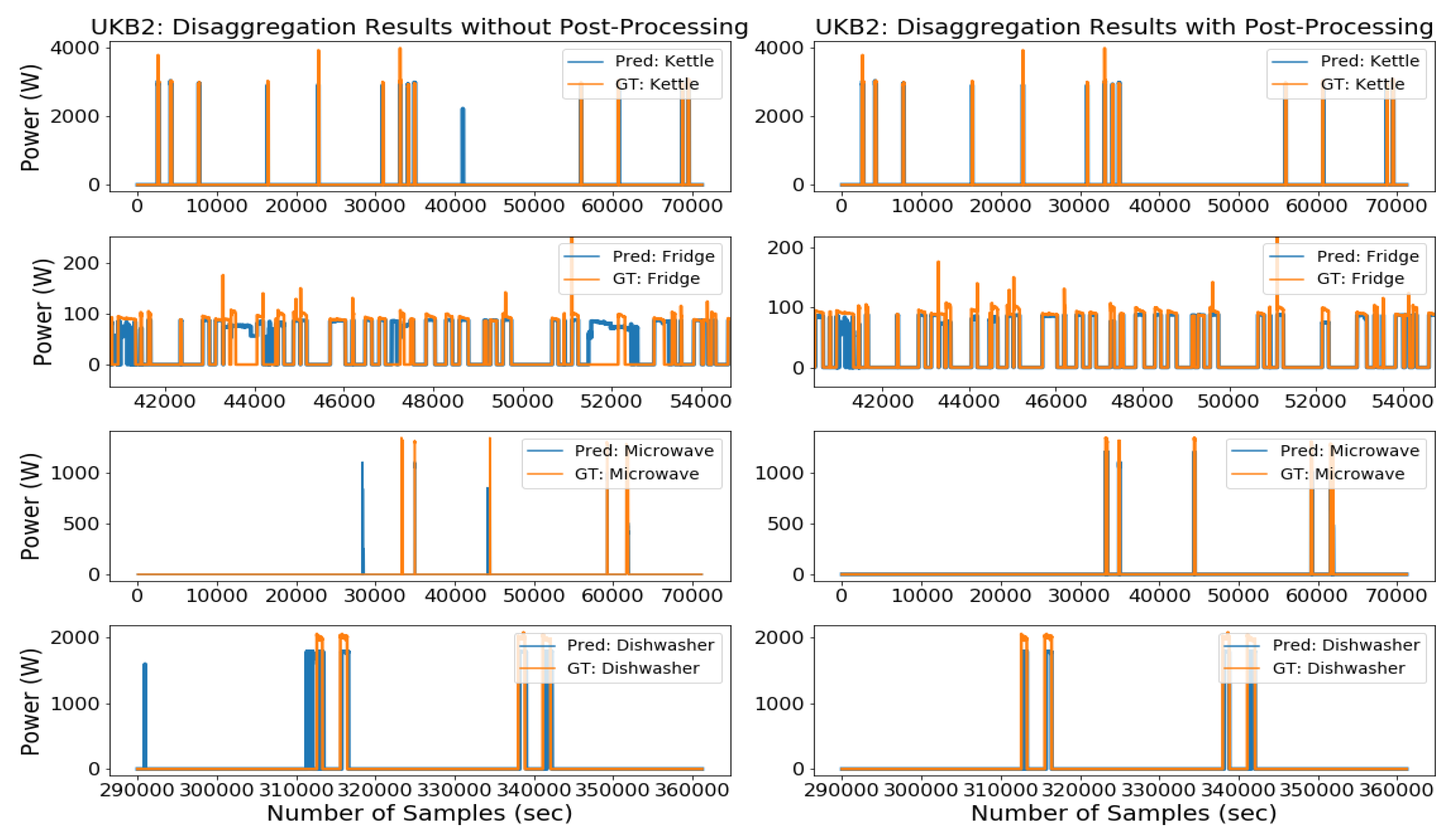
4.1.1. Results with the UKDALE Dataset

Seen scenario refers to test data, which was unseen during training. We tested individual appliance models of the kettle, microwave, dishwasher, fridge, washing machine, rice cooker, electric oven, and television on last week’s data from two houses of the UKDALE dataset. Submeter data of six appliances were taken from house-2 of the UKDALE dataset, whereas the electric oven and television data were obtained from house-5 of the UKDALE dataset. Last week’s data was unused during the training which makes it unseen data during training. Trained MFS-LSTM models for each target appliance were tested using a noised aggregated signal as input and the algorithm’s task was to predict a clean disaggregated signal for each target appliance. Figure 7 shows the disaggregation results of some of the target appliances. Visual inspection of Figure 7 shows that our proposed MFS-LSTM algorithm successfully predicted activations and energy consumption sequences of all target appliances in a given period. The proposed algorithm also predicted some irrelevant activations, which were successfully eliminated using our post-processing technique. Elimination of irrelevant activations improved precision and reduced extra predicted energy, which in turn improved classification and power estimation results of all target appliances. Numerical results of eight target appliances of UKDALE in a seen scenario are presented in

Table 2. Performance evaluation of the proposed algorithm in a seen scenario based on the UKDALE datasets.

House #	Appliances	Without Post-Processing				With Post-Processing
		F1	MAE (W)	SAE	EA	F1	MAE (W)	SAE	EA
1	Kettle	0.658	2.162	0.179	0.911	0.995	1.837	0.217	0.891
1	Fridge	0.497	13.980	0.138	0.919	0.997	5.679	0.347	0.826
5	Microwave	0.535	65.090	0.028	0.986	0.719	21.450	0.515	0.743
2	Dishwasher	0.559	13.076	0.094	0.953	0.749	5.877	0.419	0.790
1	Washing Machine	0.322	65.720	1.010	0.492	0.795	18.870	0.655	0.673
2	Electric Stove	0.886	3.519	0.623	0.688	0.981	0.240	0.005	0.997
2	Television	0.976	0.976	0.018	0.991	0.995	0.497	0.012	0.994
	Overall	0.633	23.503	0.298	0.848	0.890	7.778	0.310	0.845

. With the help of the post-processing technique, overall F1 scores (average score of all target appliances) improved from 0.688 to 0.976 (30% improvement) and MAE reduced from 23.541 watts to 8.999 watts on the UKDALE dataset. Similarly, the estimation accuracy improved from 0.714 to 0.959. Although, a significant improvement in F1-scores and MAE was observed with the use of the post-processing technique, the SAE and EA results have slightly decreased for the kettle, microwave, and dishwasher as compared to the results without post-processing. The reasons for the decrease in estimation accuracy and increase in signal aggregate error is due to the overall decrease in predicted energy after eliminating irrelevant activations.

4.1.2. Results with the ECO Dataset

The disaggregation results of seven appliances are shown in

Table 3. Performance evaluation of the proposed algorithm in a seen scenario based on the ECO datasets.

House #	Appliances	Without Post-Processing				With Post-Processing
		F1	MAE (W)	SAE	EA	F1	MAE (W)	SAE	EA
2	Kettle	0.961	3.906	0.004	0.998	0.981	2.353	0.043	0.978
2	Fridge	0.838	13.667	0.170	0.915	0.995	4.039	0.121	0.939
2	Microwave	0.721	7.285	0.276	0.862	0.869	5.402	0.437	0.781
2	Dishwasher	0.745	25.736	0.024	0.988	0.891	12.346	0.288	0.856
2	Washing Machine	0.189	30.990	0.686	−0.09	0.701	5.400	0.641	0.679
2	Rice Cooker	0.299	8.900	0.699	−0.161	0.781	1.115	0.378	0.811
5	Electric Oven	0.550	68.611	0.448	0.594	0.736	28.911	0.013	0.993
5	Television	0.512	5.695	0.219	0.890	0.879	3.428	0.649	0.675
	Overall	0.688	23.541	0.361	0.714	0.976	8.999	0.367	0.959

. These results were calculated using 1-month data which was unseen during training. Not all the appliances were present in all six houses of the ECO dataset. Kettle, fridge, and washing machine data were obtained from house-1, whereas dishwasher, electric stove, and television data were retrieved from house-2 of the ECO dataset. Similarly, microwave data were obtained from house-5 of the ECO dataset. Type-2 appliances such as the dishwasher and washing machine are very hard to classify because of various operational cycles present during their operation. With our proposed MFS-LSTM integrated with post-processing, type-2 appliances have successfully been classified and their power consumption estimation resembles ground-truth consumption according to Figure 8.

Although our algorithm was able to classify all target appliance activations, the presence of irrelevant activations in Figure 6 (left) indicates that the deep LSTM model learned some features of non-target appliances during training. This can happen due to the similar looking activation profiles of type-1 and type-2 appliances. This effect was eliminated with the use of the post-processing technique whose advantage can easily be realized with the results shown in Table 2 and Table 3 for a seen scenario.

4.2. Testing in an Unseen Scenario (Unseen Data from UKDALE House-5)

The generalization capability of our network was tested using unseen data during training. Data used for testing the algorithms was completely unseen for the trained model. In this test case, we used entire house-5 data from the UKDALE dataset for disaggregation and made sure that the testing period contains activations from all target appliances. The UKDALE dataset contains 1-sec and 6-sec sampled mains and sub-metered data, therefore, we up-sampled ground truth data to 1-sec for comparison.

Performance evaluation results of the proposed algorithm with and without post-processing in the unseen scenario are presented in

Table 4. Performance evaluation of the proposed algorithm in an unseen scenario based on the UKDALE dataset.

House #	Appliances	Without Post-Processing				With Post-Processing
		F1	MAE (W)	SAE	EA	F1	MAE (W)	SAE	EA
5	Kettle	0.701	14.973	0.685	0.657	0.965	1.966	0.058	0.971
5	Fridge	0.732	27.863	0.270	0.865	0.872	19.608	0.467	0.766
5	Microwave	0.242	0.546	0.504	0.748	0.317	0.392	0.828	0.586
5	Dishwasher	0.554	35.129	0.273	0.863	0.809	15.275	0.323	0.838
5	Washing Machine	0.189	30.990	2.18	−0.09	0.765	14.422	0.512	0.744
	Overall	0.484	21.900	0.782	0.609	0.746	10.333	0.438	0.781

. In the unseen scenario, the post-processed MFS-LSTM algorithm achieved an overall F1-score of 0.746, which was 54% better than without post-processing. Similarly, MAE reduced from 26.90W to 10.33W, SAE reduced from 0.782 to 0.438, and estimation accuracy (EA) improved from 0.609 to 0.781 (28% improvement). When MAE, SAE, and EA scores of the unseen test case were compared with the seen scenario then a visible difference in overall results was observed. One obvious reason for this difference was the different power consumption patterns of house-5 appliances; also, %-NR was higher in house-5 (72%) as compared to the house-2 noise ratio, which was 19%. However, overall results prove that the proposed algorithm can estimate the power consumption of target appliances from the seen house but can also identify appliances from a completely unseen house with unseen appliance activations.

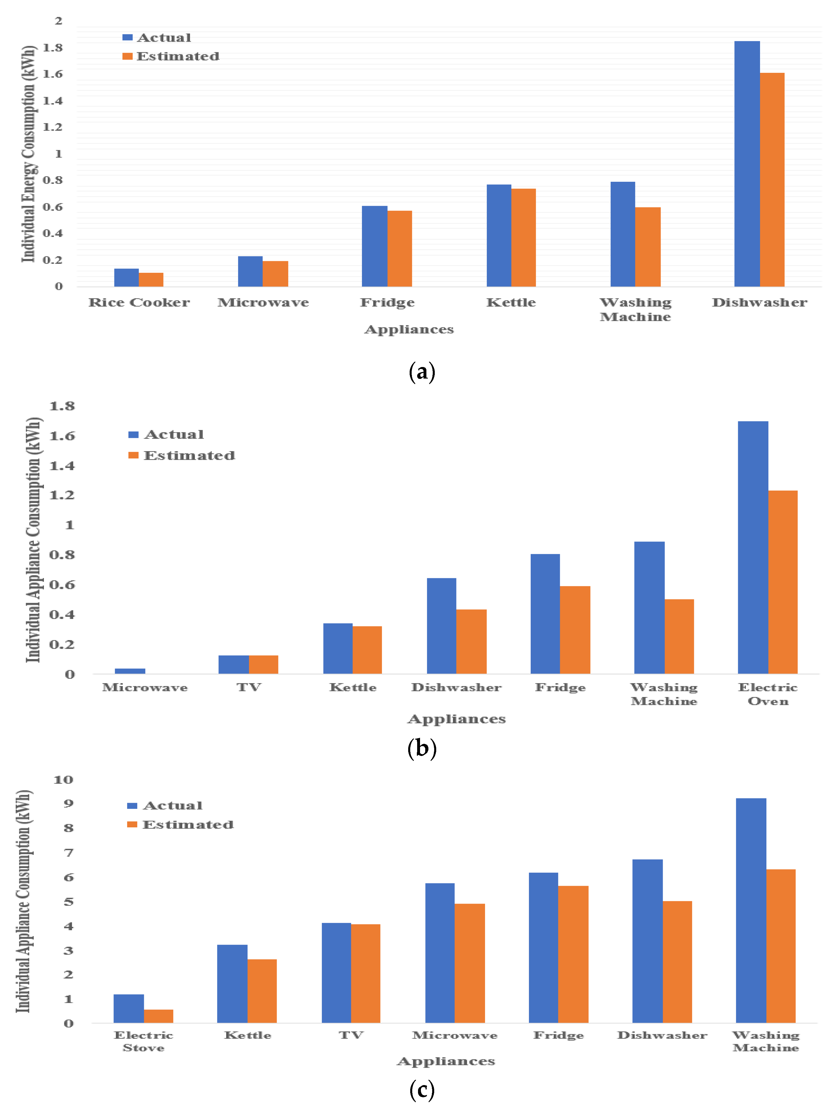
4.3. Energy Contributions by Target Appliances

Apart from individual appliance evaluation, it is also necessary to analyze total energy contributions from each target appliance. In this way, we can understand the overall performance of the algorithms when acting as a part of the NILM system. This information is helpful to analyze algorithm performance on estimating power consumption of composite appliances for a given period and how it is closely related to actual aggregated power consumption.

Figure 9 shows energy contributions from all target appliances in both seen and unseen test cases from the UKDALE and ECO datasets. The first thing to notice from Figure 9 is the amount of estimated power consumption, which is less than actual power consumption in both datasets. This happened because of the elimination of irrelevant activations which caused extra predicted energy. Another useful insight is the difference between the amount of estimated power consumption and actual consumption for type-2 appliances (dishwasher, washing machine, electric oven), which is relatively higher than the type-1 appliances difference. This could have happened due to multiple operational states of type-2 appliances which are very hard to identify as well as their power consumption is also very difficult to estimate by the DNN models. Energy contributions for all target appliances of the ECO dataset (Figure 7) are higher as compared to UKDALE appliances. This is due to the time span during which energy consumption by individual appliances was computed. For the UKDALE dataset, 1-week test data was used for evaluation. Whereas for the ECO dataset, one-month data was used for evaluation. Detailed results for energy consumption evaluation in terms of noise-ratio, percentage of disaggregated energy, and estimation accuracy are shown in

Table 5. Details of energy contributions by target appliances in UKDALE and ECO datasets.

Metrics	UKDALE H-2	UKDALE H-5	ECO H-1	ECO H-2
Noise Ratio (%)	19.34	72.08	83.76	70.51
Actual Disaggregated Energy (%)	80.66	27.92	16.24	29.49
Predicted Energy (%)	63.15	21.57	12.99	24.53
Estimation Accuracy	0.891	0.886	0.900	0.916

.

As described in Section 3.3, the noise ratio refers to energy contribution by non-target appliances. In our test cases, total energy contributions by all target appliances in said houses were 80.66%, 27.92%, 16.24%, and 79.49% respectively. Based on the results presented in Table 5, our algorithm successfully estimated power consumption of target appliances with an accuracy of 0.891 in UKDALE house-2, 0.886 in UKDALE house-5, 0.900 for ECO house-1, and 0.916 for ECO house-2.

4.4. Performance Comparison with State-of-the-Art Disaggregation Algorithms

We compared the performance of our proposed MFS-LSTM algorithm with the neural-LSTM [31], denoising autoencoder (dAE) algorithm [32], CNN based sequence-to-sequence algorithm CNN(S-S) [33], and benchmark implementations of the factorial hidden Markov model (FHMM) algorithm, and the combinatorial optimization (CO) algorithm [12] from the NILM toolkit [49]. We chose these algorithms for comparison for various reasons. First, the neural LSTM, dAE, and CNN(S-S) were also evaluated on the UKDALE dataset. Secondly, these algorithms were validated on individual appliance models as we did. Thirdly, [31,32,33] also evaluated their approach on both seen and unseen scenarios. Lastly, recent NILM works [45,54,55] have used these algorithms (CNN(S-S), CNN(S-P), neural-LSTM) to compare their approaches. That is why these three are referred to as benchmark algorithms in the NILM research.

UKDALE house-2 and house-5 data were used to train and test benchmark algorithms for seen and unseen test cases. Four-month data was used for training, whereas 10-day data was used for testing. The min-max scaling method was used to normalize the input data and individual models of five appliances were prepared for comparison. Hardware and software specifications were the same as described in Section 3.2.

Table 6. Computation time comparison between disaggregation algorithms (in seconds).

Algorithms	Training (133 Days)	Testing (10 Days)
CO	11	1.00
FHMM	166	50.63
dAE	300	0.02
Neural-LSTM	1280	0.68
CNN (S-S)	1899	1.19
MFS-LSTM	908	0.65

shows training and testing times for the above-mentioned disaggregation algorithms in terms of length of days. Many factors affect the training time of algorithms, including training samples, trainable parameters, hyper-parameters, GPU power, and complexity of the algorithm. Considering these factors, the combinatorial optimization (CO) algorithm has the lowest complexity, thus it is the fastest to execute [56]. This can also be observed from the training time of the CO algorithm from Table 6. The FHMM algorithm was the second-fastest followed by the dAE algorithm. Training time results show that the proposed MFS-LSTM algorithm has faster execution time than the neural-LSTM and CNN(S-S) because of the fewer parameters and relatively simple deep RNN architecture.

Figure 10 shows the load disaggregation comparison of the MFS-LSTM with dAE, CNN(S-S), and neural-LSTM algorithms in the seen scenario. Qualitative comparison from Figure 10 shows that the MFS-LSTM algorithm disaggregated all target appliances and proved better as compared to the dAE, neural-LSTM, and CNN(S-S) algorithms in terms of power estimation and states estimation accuracy. Although, all algorithms correctly estimated operational states of target appliances. However, the dAE algorithm showed relatively poor power estimation performance for the disaggregating kettle, fridge, and microwave. The CNN(S-S) performance was better for the disaggregating microwave. However, for all other appliances, its performance seemed to be comparative with the MFS-LSTM algorithm. These findings can be better understood through quantitative scores for all algorithms in terms of the F1 score and estimation accuracy as shown in

Table 7. Performance evaluation of disaggregation algorithms in the seen scenario.

Performance Metrics	Algorithms	Kettle	Fridge	Microwave	Dishwasher	Washing Machine	Overall
F1	CO	0.291	0.493	0.322	0.125	0.067	0.259
	FHMM	0.263	0.442	0.397	0.053	0.112	0.253
	dAE	0.641	0.735	0.786	0.746	0.485	0.679
	Neural-LSTM	0.961	0.791	0.774	0.419	0.152	0.619
	CNN(S-S)	0.940	0.912	0.923	0.708	0.759	0.848
	MFS-LSTM	0.981	0.995	0.869	0.891	0.701	0.887
MAE (Watts)	CO	61.892	53.200	59.141	71.776	121.541	73.510
	FHMM	84.270	67.244	53.472	107.655	147.330	91.994
	dAE	22.913	23.356	9.591	24.193	27.339	21.478
	Neural-LSTM	7.324	22.571	7.449	19.465	109.144	33.190
	CNN(S-S)	5.033	13.501	7.004	26.516	8.414	12.094
	MFS-LSTM	2.353	4.039	5.402	12.346	5.400	5.908
SAE	CO	0.438	0.358	0.747	0.472	0.611	0.525
	FHMM	0.463	0.516	0.849	0.594	0.523	0.589
	dAE	0.576	0.108	0.681	0.028	0.217	0.322
	Neural-LSTM	0.114	0.028	0.309	0.711	0.695	0.371
	CNN(S-S)	0.052	0.154	0.368	0.575	0.433	0.316
	MFS-LSTM	0.043	0.121	0.437	0.288	0.641	0.306
EA	CO	0.926	0.915	0.838	0.581	0.847	0.821
	FHMM	0.902	0.912	0.829	0.543	0.802	0.798
	dAE	0.711	0.946	0.659	0.986	0.723	0.805
	Neural-LSTM	0.943	0.940	0.845	0.645	0.614	0.797
	CNN(S-S)	0.972	0.930	0.717	0.723	0.745	0.817
	MFS-LSTM	0.978	0.939	0.781	0.856	0.679	0.847

.

As shown in Figure 10, the dAE’s F1 score was lower for the kettle as compared to all other algorithms. The neural-LSTM performed better in terms of the F1 score except for the dishwasher and washing machine. The CNN(S-S) performance remained comparative with the MFS-LSTM for all target appliances. The CO and FHMM algorithms showed lower state estimation accuracy compared to all other algorithms. When overall (average score) performance was considered, the MFS-LSTM achieved an overall F1 score of 0.887, which was 5% better than the CNN(S-S), 31% better than the dAE, and 43% better than the neural-LSTM and 200% better than the CO and FHMM algorithms. Considering the MAE scores, the MFS-LSTM achieved the lowest mean absolute error for all target appliances with an overall score of 5.908 watts. Only the CNN(S-S) scores were a bit close to the MFS-LSTM scores, however, the overall MAE score of the MSF-LSTM was two times less than CNN (S-S), almost four times less than the dAE, and six times less than the neural-LSTM.

Considering SAE scores, our algorithm achieved lowest SAE score of 0.043 for kettle, 0.121 for fridge, and 0.288 for dishwasher. MFS-LSTM algorithm’s consistent scores for all target appliances ensured an overall SAE score of 0.306, which was very competitive with CNN(S-S), Neural-LSTM and dAE. However, overall score of 0.306 was 71.6% lower than CO, and 92.5% lower than FHMM algorithm. When estimation accuracy scores were considered, then dAE power estimation accuracy was higher for fridge and dishwasher, and lower for microwave and washing machine. EA scores for Neural-LSTM algorithm were lower for multi-state appliances. However, MFS-LSTM algorithm achieved an overall estimation accuracy of 0.847 for being consistent in disaggregating all target appliances with high classification and power estimation accuracy.

Table 8. Performance evaluation of disaggregation algorithms in the unseen scenario.

Performance Metrics	Algorithms	Kettle	Fridge	Microwave	Dishwasher	Washing Machine	Overall
F1	CO	0.327	0.382	0.086	0.128	0.124	0.209
	FHMM	0.181	0.539	0.022	0.047	0.101	0.178
	dAE	0.746	0.671	0.432	0.652	0.415	0.583
	Neural-LSTM	0.331	0.364	0.216	0.165	0.113	0.238
	CNN(S-S)	0.783	0.684	0.226	0.495	0.533	0.544
	MFS-LSTM	0.965	0.872	0.317	0.809	0.765	0.746
MAE (Watts)	CO	113.457	89.922	77.264	81.131	77.902	87.935
	FHMM	174.744	78.511	183.472	105.626	128.756	134.222
	dAE	64.864	56.785	19.283	164.931	23.958	65.964
	Neural-LSTM	89.514	58.562	14.841	106.390	103.654	74.592
	CNN(S-S)	54.244	23.675	21.191	113.447	115.783	65.668
	MFS-LSTM	1.966	19.608	0.392	15.275	14.422	10.333
SAE	CO	0.813	0.374	0.951	0.625	0.715	0.696
	FHMM	0.871	0.569	0.982	0.754	0.763	0.788
	dAE	0.581	0.552	0.867	2.112	0.585	0.939
	Neural-LSTM	1.588	0.573	0.815	0.505	0.614	0.819
	CNN(S-S)	0.523	0.624	0.843	0.339	0.691	0.604
	MFS-LSTM	0.058	0.467	0.828	0.323	0.512	0.438
EA	CO	0.608	0.633	0.405	0.443	0.431	0.504
	FHMM	0.589	0.551	0.336	0.417	0.584	0.495
	dAE	0.709	0.724	0.566	−0.061	0.375	0.463
	Neural-LSTM	0.209	0.713	0.592	0.749	0.540	0.561
	CNN(S-S)	0.581	0.778	0.533	0.417	0.634	0.589
	MFS-LSTM	0.971	0.766	0.586	0.838	0.744	0.781

shows performance evaluation scores for benchmark algorithms in unseen scenario. F1, MAE, SAE, and estimation accuracy scores again proves effectiveness of MFS-LSTM algorithm in unseen scenario compared to benchmark algorithms. Considering F1 score, it can be observed that MFS-LSTM algorithm achieved more than 0.76 score for all target appliances except for microwave. MFS-LSTM achieved an overall score of 0.746, which was 200% better than Neural-LSTM, 27% better than CNN(S-S) and 22% better than dAE algorithm. MAE scores for MFS-LSTM were lower for all target appliances as compared to benchmark algorithms in unseen scenario. Our algorithm achieved an overall score of 10.33 watt, which was six times lower than dAE and CNN(S-S), and seven times lower than Neural-LSTM. Same trend was also observed with SAE scores, in which MFS-LSTM algorithm achieved lowest SAE scores for all target appliances except for microwave. An overall SAE score of 0.438 for MFS-LSTM algorithm was 38% lower than CNN(S-S), 59% lower than CO, 80% lower than FHMM and 87% lower than Neural-LSTM.

Estimation accuracy scores were also high for the MFS-LSTM with an overall score of 0.781. One noticeable factor is the difference in scores between the MFS-LSTM and all other algorithms in the unseen scenario. The differences shown prove the superiority of the proposed algorithm in the unseen scenario as well. Considering the noised aggregate power signal, our multi-feature input space-based approach together with post-processing can disaggregate target appliances with high power estimation accuracy as compared to state-of-the-art algorithms.

In accordance with Table 5 parameters, UKDALE house-2 and house-5 noise ratio was 19.34% and 72.08%, respectively. This implies that total predictable power was 80.66% and 27.92%. In order to estimate the percentage of predicted energy (energy contributions by all target appliances), estimation accuracy scores for all disaggregation algorithms are shown in

Table 9. Evaluation of total energy contributions by target appliances in disaggregation algorithms.

Algorithms	Estimation Accuracy (EA)
	Seen Scenario	Unseen Scenario
CO	0.907	0.544
FHMM	0.813	0.536
dAE	0.888	0.518
Neural-LSTM	0.891	0.289
CNN (S-S)	0.924	0.633
MFS-LSTM	0.964	0.856

. Presented results also highlight the proposed algorithm’s superior performance with an estimation accuracy of 0.994 and 0.956 in the seen and unseen test cases, respectively. These results suggest that our proposed algorithm efficiently estimates the power consumption of all target appliances for a given period of time.

5. Conclusions

The ultimate goal of a NILM solution is to apply it in real-time, which is possible if the disaggregation algorithm fulfills practical application requirements. Intelligent and viable disaggregation algorithms such as deep neural networks can fulfill the NILM objective if they have high estimation accuracy and lowest generalization error. However, high accuracy and lowest error are subject to the availability of a sufficient amount of training data. Recent applications of deep learning have proved that feature space exploration is a viable substitute for a high amount of data. Therefore, in order to achieve high estimation accuracy and lowest generalization error in a noised scenario, this paper proposed a multi-feature subspace-based LSTM algorithm integrated with post-processing.

First, the mutual information method was used to select those electrical features, which had a strong influence on the target appliance’s active power consumption. Based on the mutual information analysis, five electrical features were selected to form a multi-feature input space. After training individual models of nine target appliances using multi-feature input data, we tested them on unseen data from a seen house during training and unseen data from an unseen house during training in a noised scenario. The proposed MFS-LSTM algorithm successfully predicted appliance activations, along with some irrelevant activations. To eliminate those sporadic activations, we introduced a post-processing technique at the disaggregation stage. Our post-processor compared the lengths of actual and predicted activations and eliminated those activations whose lengths were less than actual activations. In order to make our solution deployable in real-time, we also proposed a three-stage NILM framework that aimed to use pre-trained appliance models (trained with the MFS-LSTM algorithm) to perform online disaggregation.

To prove our approach commendable, we compared our MFS-LSTM based deep RNN model with state-of-the-art disaggregation algorithms and accomplished an overall 66% improvement in F1-score in the seen scenario, and 120% improvement in the unseen scenario. In terms of MAE scores, we achieved 60% less error in the seen scenario and 69% less error in the unseen scenario for the MFS-LSTM algorithm. Considering SAE scores, the MFS-LSTM algorithm achieved an overall 15% less error in the seen scenario and 34% less error in the unseen scenario. Similarly, we achieved a 5% and 40% improvement in estimation accuracy in the seen and unseen test cases respectively. Results showed individual appliance performance degradation in the unseen test case due to the high percentage of noise present in the unseen test data and different power consumption patterns of the unseen target house. However, when the actual measured power and percentage of its disaggregation were considered, our proposed algorithm was able to disaggregate target appliances with more than 0.88 estimation accuracy in all target houses despite the high amount of noise present. Apart from better estimation accuracy and generalization, we also showed that the proposed algorithm is computationally efficient and its performance is independent of the increased number of appliances that make it more suitable for practical application. Future work relevant to this study will focus on training more appliances using both real and synthetic data so that trained models are generalized for various appliances having different shapes and lengths.

References

1. Zhang, G.; Wang, G.G.; Farhangi, H.; Palizban, A. Data Mining of Smart Meters for Load Category Based Disaggregation of Residential Power Consumption. Sustain. Energy Grids Netw. 2017, 10, 92–103. [Google Scholar] [CrossRef]
2. Singhal, V.; Maggu, J.; Majumdar, A. Simultaneous Detection of Multiple Appliances from Smart-Meter Measurements via Multi-Label Consistent Deep Dictionary Learning and Deep Transform Learning. IEEE Trans. Smart Grid. 2018, 10, 2969–2978. [Google Scholar] [CrossRef] [Green Version]
3. IEC. Coping with the Energy Challenge The IEC’s Role from 2010 to 2030; International Electrotechnical Commission: Geneva, Switzerland, September 2010; pp. 1–75. [Google Scholar]
4. Froehlich, J.; Larson, E.; Gupta, S.; Cohn, G.; Reynolds, M.; Patel, S. Disaggregated End-Use Energy Sensing for the Smart Grid. IEEE Pervasive Comput. 2011, 10, 28–39. [Google Scholar] [CrossRef]
5. Laitner, J.; Erhardt-Martinez, K. Examining the Scale of the Behaviour Energy Efficiency Continuum. In People-Centred Initiatives for Increasing Energy Savings; American Council for Energy Efficient Economy: Washington, DC, USA, 2010; pp. 20–31. [Google Scholar]
6. Carrie Armel, K.; Gupta, A.; Shrimali, G.; Albert, A. Is Disaggregation the Holy Grail of Energy Efficiency? The Case of Electricity. Energy Policy 2013, 52, 213–223. [Google Scholar] [CrossRef] [Green Version]
7. Paterakis, N.G.; Erdinç, O.; Bakirtzis, A.G.; Catalão, J.P.S. Optimal Household Appliances Scheduling under Day-Ahead Pricing and Load-Shaping Demand Response Strategies. IEEE Trans. Ind. Informa. 2015, 11, 1509–1519. [Google Scholar] [CrossRef]
8. De Baets, L.; Develder, C.; Dhaene, T.; Deschrijver, D. Detection of Unidentified Appliances in Non-Intrusive Load Monitoring Using Siamese Neural Networks. Int. J. Electr. Power Energy Syst. 2019, 104, 645–653. [Google Scholar] [CrossRef]
9. Zoha, A.; Gluhak, A.; Imran, M.A.; Rajasegarar, S. Non-Intrusive Load Monitoring Approaches for Disaggregated Energy Sensing: A Survey. Sensors 2012, 12, 16838–16866. [Google Scholar] [CrossRef] [Green Version]
10. Zeifman, M. Disaggregation of Home Energy Display Data Using Probabilistic Approach. IEEE Trans. Consum. Electron. 2012, 58, 23–31. [Google Scholar] [CrossRef]
11. Nalmpantis, C.; Vrakas, D. Machine Learning Approaches for Non-Intrusive Load Monitoring: From Qualitative to Quantitative Comparation. Artif. Intell. Rev. 2018, 52, 1–27. [Google Scholar] [CrossRef]
12. Hart, G.W. Nonintrusive Appliance Load Monitoring. Proc. IEEE 1992, 80, 1870–1891. [Google Scholar] [CrossRef]
13. Figueiredo, M.B.; De Almeida, A.; Ribeiro, B. An Experimental Study on Electrical Signature Identification of Non-Intrusive Load Monitoring (NILM) Systems. In Proceedings of the International Conference on Adaptive and Natural Computing Algorithms, ICANNGA, Ljubljana, Slovenia, 14–16 April 2011; pp. 31–40. [Google Scholar] [CrossRef]
14. Chang, H.H. Non-Intrusive Demand Monitoring and Load Identification for Energy Management Systems Based on Transient Feature Analyses. Energies 2012, 5, 4569–4589. [Google Scholar] [CrossRef] [Green Version]
15. Jiang, L.; Luo, S.H.; Li, J.M. Intelligent Electrical Appliance Event Recognition Using Multi-Load Decomposition. Adv. Mater. Res. 2013, 805–806, 1039–1045. [Google Scholar] [CrossRef]
16. Meehan, P.; McArdle, C.; Daniels, S. An Efficient, Scalable Time-Frequency Method for Tracking Energy Usage of Domestic Appliances Using a Two-Step Classification Algorithm. Energies 2014, 7, 7041–7066. [Google Scholar] [CrossRef] [Green Version]
17. Zeifman, M.; Roth, K. Nonintrusive Appliance Load Monitoring: Review and Outlook. IEEE Trans. Consum. Electron. 2011, 57, 76–84. [Google Scholar] [CrossRef]
18. Altrabalsi, H.; Stankovic, L.; Liao, J.; Stankovic, V. A Low-Complexity Energy Disaggregation Method: Performance and Robustness. In Proceedings of the IEEE Symposium on Computational Intelligence Applications in Smart Grid, CIASG, Orlando, FL, USA, 9–12 December 2014; pp. 1–8. [Google Scholar] [CrossRef] [Green Version]
19. Faustine, A.; Mvungi, N.H.; Kaijage, S.; Michael, K. A Survey on Non-Intrusive Load Monitoring Methodies and Techniques for Energy Disaggregation Problem. ArXiv 2017, arXiv:1703.00785. [Google Scholar]
20. Esa, N.F.; Abdullah, M.P.; Hassan, M.Y. A Review Disaggregation Method in Non-Intrusive Appliance Load Monitoring. Renew. Sustain. Energy Rev. 2016, 66, 163–173. [Google Scholar] [CrossRef]
21. Kolter, J.Z.; Johnson, M.J. REDD: A Public Data Set for Energy Disaggregation Research. In Proceedings of the ACM Workshop on Data Mining Applications in Sustainability (SustKDD), San Diego, California, 21 August 2011; pp. 1–6. [Google Scholar]
22. Kolter, Z.; Jaakkola, T.; Kolter, J.Z. Approximate Inference in Additive Factorial HMMs with Application to Energy Disaggregation. J. Mach. Learn. Res. 2012, 22, 1472–1482. [Google Scholar]
23. Zoha, A.; Gluhak, A.; Nati, M.; Imran, M.A. Low-Power Appliance Monitoring Using Factorial Hidden Markov Models. In Proceedings of the 2013 IEEE 8th International Conference on Intelligent Sensors, Sensor Networks and Information Processing: Sensing the Future, ISSNIP 2013, Melbourne, Australia, 2–5 April 2013; Volume 1, pp. 527–532. [Google Scholar] [CrossRef] [Green Version]
24. Bonfigli, R.; Principi, E.; Fagiani, M.; Severini, M.; Squartini, S.; Piazza, F. Non-Intrusive Load Monitoring by Using Active and Reactive Power in Additive Factorial Hidden Markov Models. Appl. Energy 2017, 208, 1590–1607. [Google Scholar] [CrossRef]
25. Ruzzelli, A.G.; Nicolas, C.; Schoofs, A.; O’Hare, G.M.P. Real-Time Recognition and Profiling of Appliances through a Single Electricity Sensor. In Proceedings of the SECON 2010—2010 7th Annual IEEE Communications Society Conference on Sensor, Mesh and Ad Hoc Communications and Networks, Boston, MA, USA, 21–25 June 2010. [Google Scholar] [CrossRef] [Green Version]
26. Lin, G.Y.; Lee, S.C.; Hsu, J.Y.J.; Jih, W.R. Applying Power Meters for Appliance Recognition on the Electric Panel. In Proceedings of the 2010 5th IEEE Conference on Industrial Electronics and Applications, ICIEA 2010, Taichung, Taiwan, 15–17 June 2010; pp. 2254–2259. [Google Scholar] [CrossRef]
27. Mauch, L.; Yang, B. A New Approach for Supervised Power Disaggregation by Using a Deep Recurrent LSTM Network. In Proceedings of the 2015 IEEE Global Conference on Signal and Information Processing, GlobalSIP 2015, Orlando, FL, USA, 14–16 December 2015; pp. 63–67. [Google Scholar] [CrossRef]
28. Rafiq, H.; Zhang, H.; Li, H.; Ochani, M.K. Regularized LSTM Based Deep Learning Model: First Step towards Real-Time Non-Intrusive Load Monitoring. In Proceedings of the IEEE International Conference on Smart Energy Grid Engineering (SEGE), Oshawa, ON, Canada, 12–15 August 2018; pp. 234–239. [Google Scholar] [CrossRef]
29. He, W.; Chai, Y. An Empirical Study on Energy Disaggregation via Deep Learning. Adv. Intell. Syst. Res. 2016, 133, 338–342. [Google Scholar] [CrossRef] [Green Version]
30. Kim, J.; Le, T.-T.-H.; Kim, H. Nonintrusive Load Monitoring Based on Advanced Deep Learning and Novel Signature. Comput. Intell. Neurosci. 2017, 2017, 4216281. [Google Scholar] [CrossRef]
31. Kelly, J.; Knottenbelt, W. Neural NILM: Deep Neural Networks Applied to Energy Disaggregation. In Proceedings of the ACM International Conference on Embedded Systems for Energy-Efficient Built Environments, Seoul, South Korea, 3–4 November 2015; pp. 55–64. [Google Scholar] [CrossRef] [Green Version]
32. Bonfigli, R.; Felicetti, A.; Principi, E.; Fagiani, M.; Squartini, S.; Piazza, F. Denoising Autoencoders for Non-Intrusive Load Monitoring: Improvements and Comparative Evaluation. Energy Build. 2018, 158, 1461–1474. [Google Scholar] [CrossRef]
33. Zhang, C.; Zhong, M.; Wang, Z.; Goddard, N.; Sutton, C. Sequence-to-Point Learning with Neural Networks for Nonintrusive Load Monitoring. In Proceedings of the Thirty-Second AAAI Conference on Artificial Intelligence, New Orleans, LA, USA, 2–7 February 2018; pp. 1–8. [Google Scholar]
34. Barsim, K.S.; Yang, B. On the Feasibility of Generic Deep Disaggregation for Single-Load Extraction. ArXiv 2018, arXiv:1802.02139. [Google Scholar]
35. Zhang, Y.; Yin, B.; Cong, Y.; Du, Z. Multi-state Household Appliance Identification Based on Convolutional Neural Networks and Clustering. Energies 2020, 13, 792. [Google Scholar] [CrossRef] [Green Version]
36. D’Incecco, M.; Squartini, S.; Zhong, M. Transfer Learning for Non-Intrusive Load Monitoring. IEEE Trans. Smart Grid 2020, 11, 1419–1429. [Google Scholar] [CrossRef]
37. Singh, S.; Majumdar, A. Deep Sparse Coding for Non-Intrusive Load Monitoring. IEEE Trans. Smart Grid 2018, 9, 4669–4678. [Google Scholar] [CrossRef] [Green Version]
38. Cho, J.; Hu, Z.; Sartipi, M. Non-Intrusive A/C Load Disaggregation Using Deep Learning. In Proceedings of the IEEE Power Engineering Society Transmission and Distribution Conference, Denver, CO, USA, 16–19 April 2018; pp. 1–5. [Google Scholar] [CrossRef]
39. Miao, J.; Niu, L. A Survey on Feature Selection. Procedia Comput. Sci. 2016, 91, 919–926. [Google Scholar] [CrossRef] [Green Version]
40. Masoudi-Sobhanzadeh, Y.; Motieghader, H.; Masoudi-Nejad, A. FeatureSelect: A Software for Feature Selection Based on Machine Learning Approaches. BMC Bioinformatics 2019, 20, 170. [Google Scholar] [CrossRef]
41. Zhu, Z.; Wei, Z.; Yin, B.; Liu, T.; Huang, X. Feature Selection of Non-Intrusive Load Monitoring System Using RFE and RF. J. Phys. Conf. Ser. 2019, 1176, 1–8. [Google Scholar] [CrossRef]
42. Schirmer, P.A.; Mporas, I. Statistical and Electrical Features Evaluation for Electrical Appliances Energy Disaggregation. Sustainability 2019, 11, 3222. [Google Scholar] [CrossRef] [Green Version]
43. Valenti, M.; Bonfigli, R.; Principi, E.; Squartini, S. Exploiting the Reactive Power in Deep Neural Models for Non-Intrusive Load Monitoring. In Proceedings of the International Joint Conference on Neural Networks, Rio de Janeiro, Brazil, 8–13 July 2018; 2018; pp. 1–8. [Google Scholar] [CrossRef]
44. Harell, A.; Makonin, S.; Bajic, I.V. Wavenilm: A Causal Neural Network for Power Disaggregation from the Complex Power Signal. In Proceedings of the ICASSP, IEEE International Conference on Acoustics, Speech and Signal Processing—Proceedings, Brighton, UK, 12–17 May 2019. [Google Scholar] [CrossRef] [Green Version]
45. Kong, W.; Dong, Z.Y.; Wang, B.; Zhao, J.; Huang, J. A Practical Solution for Non-Intrusive Type II Load Monitoring Based on Deep Learning and Post-Processing. IEEE Trans. Smart Grid 2020, 11, 148–160. [Google Scholar] [CrossRef]
46. Beraha, M.; Metelli, A.M.; Papini, M.; Tirinzoni, A.; Restelli, M. Feature Selection via Mutual Information: New Theoretical Insights. In Proceedings of the International Joint Conference on Neural Networks (IJCNN), Budapest, Hungary, 14–19 July 2019; pp. 1–9. [Google Scholar] [CrossRef] [Green Version]
47. Tabatabaei, S.M. Decomposition Techniques for Non-Intrusive Home Appliance Load Monitoring; University of Alberta: Edmonton, AB, Canada, 2014. [Google Scholar] [CrossRef]
48. Asif, W.; Rajarajan, M.; Lestas, M. Increasing User Controllability on Device Specific Privacy in the Internet of Things. Comput. Commun. 2018, 116, 200–211. [Google Scholar] [CrossRef] [Green Version]
49. Batra, N.; Kelly, J.; Parson, O.; Dutta, H.; Knottenbelt, W.; Rogers, A.; Singh, A.; Srivastava, M. NILMTK: An Open Source Toolkit for Non-Intrusive Load Monitoring Categories and Subject Descriptors. In Proceedings of the International Conference on Future Energy Systems (ACM e-Energy), Cambridge, UK, 11–13 June 2014; pp. 1–4. [Google Scholar] [CrossRef] [Green Version]
50. Kelly, J.; Knottenbelt, W. The UK-DALE Dataset, Domestic Appliance-Level Electricity Demand and Whole-House Demand from Five UK Homes. Sci. Data 2015, 2, 150007. [Google Scholar] [CrossRef] [PubMed] [Green Version]
51. Beckel, C.; Kleiminger, W.; Cicchetti, R.; Staake, T.; Santini, S. The ECO Data Set and the Performance of Non-Intrusive Load Monitoring Algorithms. In Proceedings of the 1st ACM Conference on Embedded Systems for Energy-Efficient Buildings—BuildSys ’14, Memphis, TN, USA, 5–6 November 2014; pp. 80–89. [Google Scholar] [CrossRef]
52. Chollet, F. Keras: The Python Deep Learning Library. Available online: https://keras.io (accessed on 8 April 2020).
53. Makonin, S.; Popowich, F. Nonintrusive Load Monitoring (NILM) Performance Evaluation A Unified Approach for Accuracy Reporting. Energy Effic. 2015, 8, 809–814. [Google Scholar] [CrossRef]
54. Gomes, E.; Pereira, L. PB-NILM: Pinball Guided Deep Non-Intrusive Load Monitoring. IEEE Access 2020, 8, 48386–48398. [Google Scholar] [CrossRef]
55. Xia, M.; Liu, W.; Wang, K.; Zhang, X.; Xu, Y. Non-Intrusive Load Disaggregation Based on Deep Dilated Residual Network. Electr. Power Syst. Res. 2019, 170, 277–285. [Google Scholar] [CrossRef]
56. Manivannan, M.; Najafi, B.; Rinaldi, F. Machine Learning-Based Short-Term Prediction of Air-Conditioning Load through Smart Meter Analytics. Energies 2017, 11, 1905. [Google Scholar] [CrossRef] [Green Version]
Figure 1. Proposed architecture of the three-stage multi-feature input space (MFS)- long short-term memory (LSTM) algorithm.
Energies 13 02195 g001
Figure 2. A single recurrent neural networks (RNN) unit showing LSTM architecture.
Energies 13 02195 g002
Figure 3. An example of predicted energy sequence of (a) dishwasher and (b) microwave showing the presence of irrelevant activations with a zoomed-in view of irrelevant activation shape and length that does not correspond to ground-truth activation.
Energies 13 02195 g003aEnergies 13 02195 g003b
Figure 4. Real-time deployable NILM framework employing MFS-LSTM algorithm.
Energies 13 02195 g004
Figure 5. Normalized mutual information scores between various electrical features and target appliance power consumption.
Energies 13 02195 g005
Figure 6. Effects of different hyperparameters on the learning behavior of the MFS-LSTM. (a) the learning behavior with varying layer widths corresponding to the first layer. (b) the influence of the layer width on the training and validation loss. (c) the influence of the learning rate on the training loss. (d) the impact of the activation function on learning behavior.
Energies 13 02195 g006
Figure 7. Seen Scenario—Disaggregation results of some target appliances from the UKDALE dataset with and without post-processing.
Energies 13 02195 g007
Figure 8. Seen Scenario: Disaggregation results of all target appliances from the ECO dataset
Energies 13 02195 g008
Figure 9. Energy contributions by individual appliances from (a) UKDALE House-2, (b) UKDALE House-5, (c) ECO House-1 and 2.
Energies 13 02195 g009
Figure 10. Comparison of disaggregation algorithms in the seen scenario based on the UKDALE dataset.
Energies 13 02195 g010