Route Guidance Strategies for Electric Vehicles by Considering Stochastic Charging Demands in a Time-Varying Road Network


1
School of Traffic and Transportation, Beijing Jiaotong University, Beijing 100044, China
2
Key Laboratory of Transport Industry of Big Data Application Technologies for Comprehensive Transport, Beijing Jiaotong University, Beijing 100044, China
3
Department of Civil and Environmental Engineering, Norwegian University of Science and Technology, 7033 Trondheim, Norway
*
Author to whom correspondence should be addressed.
Energies 2020, 13(9), 2287; https://0-doi-org.brum.beds.ac.uk/10.3390/en13092287
Submission received: 2 February 2020
/
Revised: 27 April 2020
/
Accepted: 28 April 2020
/
Published: 5 May 2020
(This article belongs to the Special Issue Electric Systems for Transportation)
Abstract
:Electric vehicles (EVs) are being increasingly adopted because of global concerns about petroleum dependence and greenhouse gas emissions. However, their limited driving range results in increased charging demands with a stochastic characteristic in real-world situations, and the charging demands should be attributed toward charging stations in time-varying road networks. To this end, this study proposes guidance strategies to provide efficient choice for charging stations and corresponding routes, and it includes the time-varying characteristic of road networks in problem formulation. Specifically, we propose two route guidance strategies from different perspectives based on the charging demand information. The first strategy focuses on the effects of the number of EVs on the charging stations’ operation, and the reachable charging stations with the fewest vehicles are selected as the heuristic suggested ones. The other strategy considers the travel cost of individual drivers and selects the charging stations nearest to the destination as heuristic suggested ones. Both strategies ensure that the selected charging stations can be reached in a time-varying road network. In addition, we carry out a simulation analysis to investigate the performance of the proposed route guidance strategies and introduce relevant insights and recommendations for the application of the strategies under various scenarios.
1. Introduction
Dependence on petroleum contributes to a serious environmental and energy problem. The transportation sector is one of the major economic industries that contribute to energy consumption and greenhouse gas emissions. The International Energy Agency found that the transportation sector contributes 28% of global energy consumption and 23% of global greenhouse gas emissions [1]. Electric vehicles (EVs), which are highly energy-efficient, are recognized as a promising solution to alleviate the problem of fossil fuel dependency and increasing greenhouse gas emissions, especially if the energy used for their charging is obtained from a renewable energy source [2]. However, unlike conventional internal combustion engine vehicles, EVs have a relatively short driving range because of their limited battery capacity, thus requiring drivers to recharge their vehicles often to reach their destinations. Insufficient charging infrastructure often causes difficulties in finding charging stations, thus resulting in the range anxiety of EV drivers [3]. Range anxiety can be effectively alleviated by providing guidance information for EV charging based on specific service platforms, such as a smart charging service. Drivers could file charging demands to the charging service provider and receive recommended charging stations through their mobile devices [4]. Guidance strategies should be developed in consideration of charging demand information to determine the recommended charging stations and corresponding travel routes. The traffic condition on a road network also affects the route choice of EVs from departure points to charging stations, because the traffic volume would vary as time progresses in real-world situations, due to the factors such as rush hour, which is regarded as the time-varying characteristic for a road network [5]. Such a characteristic would influence vehicle driving state and should be considered in the route guidance strategies. The stochastic characteristic intrinsic to the charging demands substantially affects the strategies, thus further increasing the difficulty of dealing with charging demands. Large-scale charging behaviors with stochastic characteristics considerably affect the operation efficiency of charging stations. Therefore, given the widespread adoption of EVs, solving stochastic charging demands in complex real-world situations is a critical issue for the current and future global transportation system.
Directing EVs to suitable charging stations is an important and fundamental problem for the adoption of EVs in urban transportation systems. As introduced in Section 2, the traditional methods of route guidance for EVs mainly focus on the problems with deterministic charging demands in a static road network. Although several studies considered the impacts of a time-varying road network on the driving state of vehicles, less attention was paid to the stochastic characteristics intrinsic to charging demands. Therefore, a route guidance method that can be used to deal with stochastic charging demands and that takes into account the time-varying road network is expected. To fill the gap, this study develops route guidance strategies for stochastic charging demands in a time-varying road network from two different perspectives. The performance of the route guidance strategies is explored by considering their effects on the operation efficiency of charging stations. Both strategies can direct EVs with stochastic charging demands to reachable charging stations by considering the time-varying traffic conditions on the routes.
This study makes the following unique contributions: firstly, the stochastic characteristic of charging demands is investigated given the situation with large-scale adoption of EVs. A route guidance problem with stochastic charging demands is formulated by combining the time-varying road network. A dynamic recursive equation is developed to obtain the EV number in charging stations, which varies as time progresses. Secondly, to address stochastic charging demands, two route guidance strategies are established, and the operation efficiency of charging stations and travel cost of individual drivers are considered in the strategies. In actual situations, the operation efficiency of charging stations could be affected by the number of EVs in them, because the sustainable number of EVs for a charging station is limited and the queuing time is increased as vehicle number increases. Therefore, we use the number of EVs in charging stations as the matric to reflect the operation efficiency of charging stations. In addition, the travel cost of individual drivers is generally composed of travel time, energy consumption, and charging cost. These travel cost components are closely correlated with driving distance. Thus, the driving distance is employed to reflect the integration of travel cost components. The reachability of the selected charging stations can be ensured by both strategies in a time-varying road network. Lastly, the proposed strategies are applied in simulation examples to provide guidance for stochastic charging demands in a time-varying road network. The performance of the two strategies is compared in different simulation scenarios, and application recommendations in terms of the strategies are presented based on the simulation results.
The remaining portions of this paper are arranged as follows: in Section 2, the literature review is presented. In Section 3, the route guidance problem is formulated by considering the stochastic charging demands in a time-varying road network. In Section 4, the metrics regarding the charging station selection are analyzed from two different perspectives, and the route guidance strategies are presented. In Section 5, the simulated results are presented to compare the performance of the proposed strategies. Lastly, the conclusions and future studies are discussed in Section 6.
2. Literature Review
EVs are a potential solution to environmental and energy problems because they have high energy efficiency and can be charged by using renewable energy source. Thus, the traveling and charging problems of EVs attracted increasing interest from the scientific community. Given the limited driving range of EVs, several studies attempted to find optimal routes for EVs on the basis of the framework of the constrained shortest path problem [6,7,8]. However, charging behavior was not involved in the methods. Considering the charging demands incurred by EV travels, Wang et al. used geometric approaches and designed an algorithm for route guidance by considering the charging demand information from drivers [4]. Driving direction and distance were used as choice indicators for optimal charging stations. Sweda et al. proposed two heuristic methods for making adaptive routing and recharging decisions for EVs [9]. Charging costs were involved in the solution. In addition to charging processes, Qin and Zhang and Said et al. considered the effects of queuing time on charging station selection [10,11]. Queuing theory was used to optimize the route guidance. Several studies combined driving time, charging time, and queuing time to discuss charging and route optimization for EVs [12,13,14]. Wang et al. incorporated energy constraints during travel and proposed an energy-aware routing model for EVs [15]. Cao et al. and Liu et al. considered the effects of charging costs on charging station selection to investigate EV charging problems [16,17]. Yagcitekin and Uzunoglu developed a smart route guidance strategy based on double-layer optimization theory [18]. Sun and Zhou compared the effects of different factors on route selection of EVs by using a cost-optimal algorithm [19]. The trade-off between traveling cost and time consumed was obtained to guide drivers in traveling and charging. Wang et al. integrated drivers’ intended traveling and charging choices [20]. A multiobjective model was established to provide guidance for EV charging; the objectives include minimized traveling time, charging costs, and energy consumption. In view of the environmental effects for EV adoption, many studies aimed to search for energy-efficient routes for EVs under different situations [21,22,23,24,25]. However, the aforementioned methods for route guidance are mainly based on problems in a static road network, in which the time or energy consumed in each link is constant. Consequently, the effects of traffic condition on driving state are ignored, which makes the solution unrealistic in complex situations with respect to urban road networks.
In view of this, Alizadeh et al. incorporated time-varying traffic conditions in the traveling and charging problems for EVs to improve the accuracy of route guidance schemes [26]. An extended transportation graph was used to find the optimal routes. Yi and Bauer proposed a model to investigate the effects of traffic condition on energy cost of EVs [27]. The primal–dual interior point algorithm was used to construct the optimal paths. Zhang et al. proposed a multiobjective routing model for EV travel, in which the effects of traffic condition on travel time, driving distance, and energy consumption were considered [28]. The ant colony optimization algorithm was employed to search for optimal routes. Jafari and Boyles incorporated route reliability in the solution for an EV traveling problem under a road network with time-varying traffic condition [29]. Daina et al. explored the EV charging problem by considering uncertain traffic conditions on the basis of random utility theory [30]. The trade-off among driving distance, charging time, and costs for charging selection was analyzed. Huber and Bogenberger utilized real-time traffic information to investigate the time-varying characteristic of traffic conditions and their effects on the EV driving state [31]. Several works introduced network equilibrium theory to explore the optimization models for EV charging and traveling [32,33,34,35]. They modeled changing traffic conditions by changing the number of vehicles in each link. However, most existing methods assume that the charging demands of EV drivers are predetermined and overlook their stochastic characteristics. In real-world situations, charging demands with variable information may be made at different periods, and the charging service providers are unable to know the information before they receive the charging demands. Therefore, the previous methods are unable to solve stochastic charging demands in complex real-world situations.
Furthermore, to address stochastic charging demands, Hung and Michailidis proposed a route guidance strategy based on the queuing modeling framework, in which charging demands occur in accordance with a general process during a time period [36]. Nevertheless, the study did not consider the time-varying characteristic of road networks. EVs were assumed to operate with a constant speed in the road network. Energy consumption, which considerably influences the reachability of charging stations, was also ignored in the method. To our knowledge, few studies investigated the route guidance methods of EVs by comprehensively considering stochastic charging demands and a time-varying road network.
Overall, even though the previous studies made achievements in route guidance for EVs, there are still some limitations, as mentioned above. To further clarify the existing studies, we summarize the aforementioned references with respect to their considerations, as listed in Table 1 (considered factors are marked as “√”; otherwise, unconsidered factors are marked as “×”). In view of the limitations, two heuristic-based strategies for route guidance are proposed and introduced in the following sections, which aim to deal with stochastic charging demands in a time-varying road network.
3. Problem Description
During trips, EV drivers often need to recharge their vehicles to reach their destinations, thus resulting in charging demands in a road network with EVs. The charging demand information is assumed to include drivers’ travel destinations and the remaining energy of vehicles. Travel destination is one of the critical factors in drivers’ travel demand. The remaining energy of EVs can be directly obtained through built-in vehicle dashboards. When EV drivers notice that the remaining energy of their vehicle may be insufficient to reach their destinations, they send the information of charging demands to the charging service provider by using their mobile devices. When receiving charging demands from EV drivers, the charging service provider needs to determine the suitable charging station for each charging demand according to the given information. Note that charging demands in real-world situations have uncertainty and variability by time. That is, the charging demands received in different periods may contain different information about travel destinations of drivers and the remaining energy of EVs. Specifically, both travel destinations and remaining energy have uncertainty from the perspective of the charging service provider, because they derive from the individual travel demands of drivers and operation state of EVs, respectively, thus preventing the charging service provider from predicting the detailed information of charging demands in advance. In situations with large-scale charging demands, multiple charging demands during identical periods often have different information on travel destinations and remaining energy. In actual situations, the charging service provider can obtain the information on EV and charging station locations by using positioning devices. EV drivers do not need to send the location information to the charging service provider, whether the charging demands occur or their detailed information is not predetermined at different periods. Thus, the charging demands in a road network have a significant stochastic characteristic as time progresses. To realize problem formulation, the time is discretized into finite time slots normalized to integral units. Let denote the set of time slots, where T is the total number of the time slots. With the identical duration for each time slot, the time horizon increases as T increases. The charging demand that occurs in node i and at time slot t is denoted by , which is a binary variable in the problem formulation. Its value is equal to 1 if there exists a charging demand that occurs in normal node i at time slot t; otherwise, it is equal to 0. For each charging demand , its information includes the travel destination and remaining energy, which are denoted as and , respectively. The travel destination and remaining energy from different charging demands may vary. The charging service provider cannot understand or predict before time slots t. Thus, the decision-making for all the charging demands needs to be determined based on the traffic condition at corresponding time slots.
The stochastic characteristic of charging demands is one of the challenges in situations with large-scale adoption of EVs. Traffic conditions in a road network also affect the driving speed and energy consumption of EVs, thus affecting their traveling and charging process [37]. Traffic conditions often have time-varying characteristic in real-world situations because of environmental factors [38]. Consequently, the energy and time that are spent while traversing the same links may vary at different time slots. The time-varying characteristic of a road network should be considered to improve the effectiveness of route guidance schemes. The road network structure and EV operating characteristics are combined, and the time-varying road network is defined as , where V and A denote the sets of nodes and links, respectively. In set V, two types of nodes, namely, normal and charging station nodes, exist. The latter has the ability to charge EVs. For problem formulation, set V is assumed to consist of m normal nodes and n charging station nodes. and in G denote the driving time and energy consumption on link a at time slot t, respectively, where . In every time slot, the values of and randomly change within a reasonable range, which reflects the time-varying characteristic of the road network. The conventional optimization problems with time-varying networks often assume that the links remain stable for the duration of a time slot [39]. For the problem of route guidance for EV charging, the assumption signifies the constant driving time and energy consumption during a separate time slot. The assumption conforms to the traffic condition characteristic in an actual road network if the duration for each time slot is relatively short. Therefore, we follow such an assumption in the route guidance problem for EV charging.
The route guidance problem for EV charging is formulated by combining stochastic charging demands and time-varying road networks. The charging demands are assumed to occur in the normal nodes only. The charging station nodes could not generate charging demands. Such an assumption is reasonable, because drivers seek help from the charging service provider only when they have difficulty finding nearby charging stations. The guidance strategies aim to help EV drivers from normal nodes select heuristic suggested charging station nodes based on specific objectives. The binary decision variable in the problem formulation is denoted by , which is equal to 1 if the charging demand generated in normal node i at time slot t is assigned to charging station node j ; otherwise, this variable is 0. In every time slot, all the normal nodes in a road network have the potential to generate charging demands. However, whether the charging demands occur or not in every time slot is an uncertain event. In order to reflect such a characteristic of charging demand occurrence, the possibility of the charging demand occurring in node i at each time slot is denoted as , as shown in Equation (1).
where Pr (Λ) represents the possibility of the occurrence of event Λ.
Note that, given the definition of charging demand occurrence as shown in Equation (1), we assume that each normal node is able to generate at most one charging demand following a specific possibility during a time slot. The assumption conforms to the characteristic of charging demand occurrence in actual situations if the duration for each time slot is relatively short. Moreover, to reduce the complexity of problem formulation, we assume that the charging demand occurrence for each node follows a uniform distribution. For example, the possibility of charging demand occurrence for node i has a uniform value as time progresses, which does not have a time-varying characteristic and is influenced by the node location. Although node i has a constant possibility for every time slot, the travel destination and remaining energy from the charging demands may vary at different time slots.
When addressing the charging demands at each time slot, the first step is to ensure that the remaining energy can enable the EVs to reach the target charging stations. In a time-varying road network, the energy consumption between normal and charging station nodes may vary at different time slots. Thus, before charging stations are selected, the energy consumption on the routes should be observed, and only the reachable charging stations can be considered as candidates, as shown in Figure 1.
In Figure 1, the energy consumptions between node 1 and CS 1 at time slots t1 and t2 are different. The green check mark indicates that the EV can traverse the route, and the red cross indicates that the EV cannot do so because it has insufficient remaining energy. The figure indicates that the reachability of the same charging station may vary at different time slots because of the time-varying traffic conditions on the road network. The driving time on the routes may also change at different time slots, thus determining the suitable time slots as the EVs reach charging stations. The charging service provider is assumed to know the information about the traffic conditions on all the links at the beginning of each time slot, acquiring such information through either real-time traffic information from the transport sector or short-term traffic flow prediction [40]. The basic framework for the stochastic route guidance problem in a time-varying road network is presented in Figure 2.
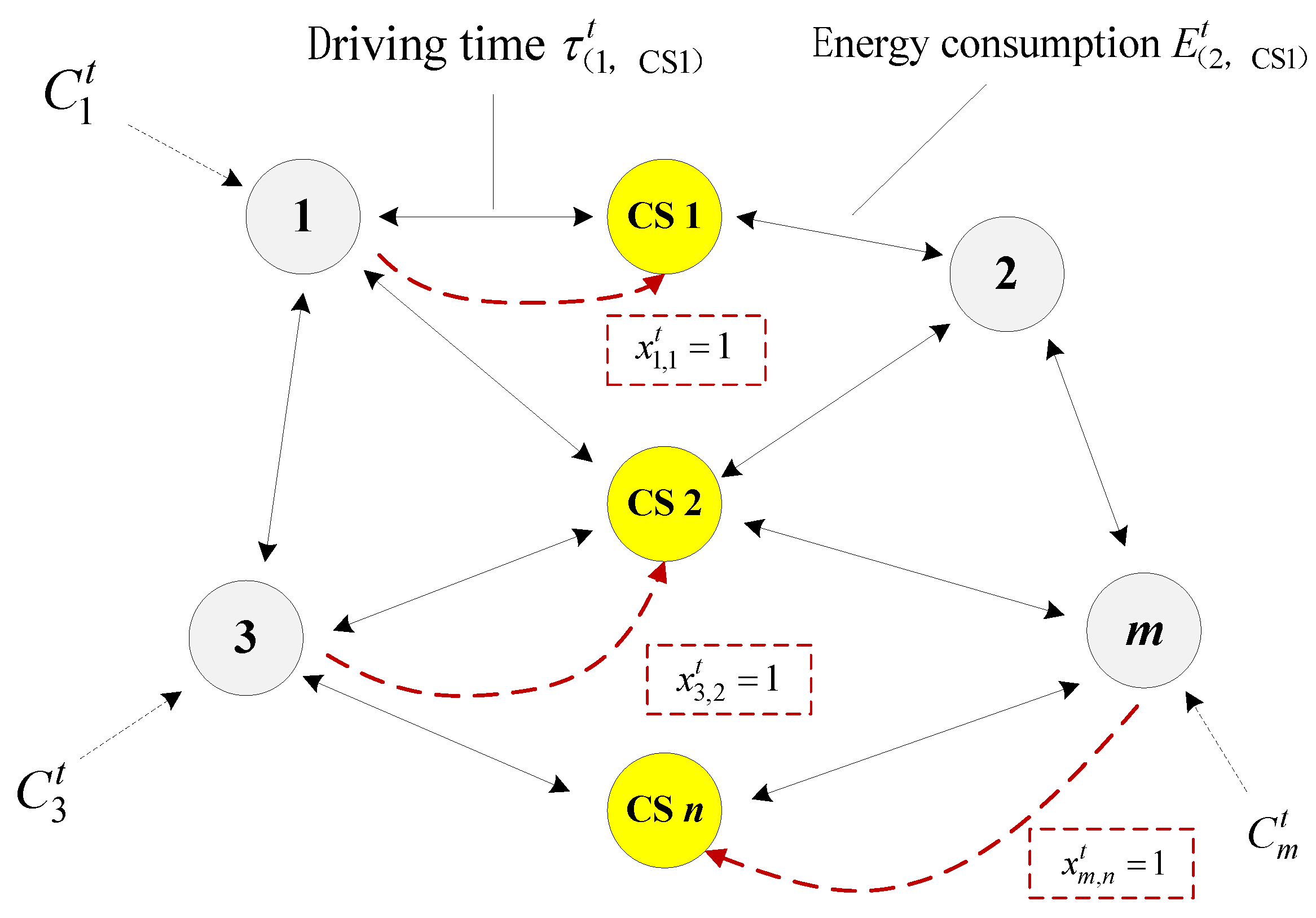
In Figure 2, is the driving time from node 1 to charging station node CS 1 under the traffic condition at time slot t. The energy consumption between node 2 and charging station node CS 1 at time slot t is denoted by . The charging demands that occur in nodes 1, 3, and m at time slot t are denoted as , , and , respectively. The objective of the problem is to provide guidance for every charging demand by considering the traffic condition at time slot t. The recommended charging station nodes would be selected for the charging demands based on specific route guidance strategies. In the figure, the decision for charging station selection is denoted as , , and . For instance, indicates that the charging demand that occurs in node 1 is assigned to the charging station node CS 1. How to determine the value of at each time slot t is the critical issue to solve the route guidance problem for EV charging in a time-varying road network. This issue should be considered from two aspects. Firstly, the route guidance strategies satisfy the charging demands of EV drivers; that is, an EV should be able to reach the selected charging station under its current remaining energy. For this reason, the relationship between remaining energy and traffic condition needs to be considered. Secondly, the charging behavior has significant effects on the operating state of charging stations, especially in a situation with large-scale adoption of EVs. In every time slot, multiple charging demands may occur in a road network, and the charging stations may have to accept multiple EVs. Given the limited charging rate, the number of EVs in a charging station increases as the time slots pass. However, mass EV charging significantly affects the operating state of charging stations; that is, it may prolong the queuing time and even present a potential burden on local power systems [41,42,43]. Therefore, aside from drivers’ charging demands, the number of EVs at each charging station is another important factor that needs to be considered by route guidance strategies.
We attempt to develop a dynamic recursive equation based on the operation characteristics of charging stations to explore the change trend of EV number in charging stations under the situation with large-scale stochastic charging demands. denotes the number of EVs that complete charging and leave charging station j at time slot t. Without loss of generality, the problem assumes that at most one EV can leave a charging station after completing charging at each time slot. The assumption conforms to the actual operating situation in charging stations if the duration for each time slot is relatively short. The possibility of the event that an EV leaves the charging station j after completing charging at each time slot is denoted as , as shown in Equation (2).
The parameter can reflect the charging levels of the chargers in charging station j. During the actual charging processes, the chargers with different charging levels have different charging rates for EVs [44]. Under the definition of and , the duration between two adjacent events of an EV leaving charging station j follows a geometric distribution [45]. The EV number in charging station j at time slot t is denoted by . The dynamic recursive equation for is
where represents the initial EV number in charging station j within a specific time horizon, and is the time slot when the charging demand from node i occurs. In the equation, the time slots and satisfy the following relationship:
Equation (4) indicates that the EV with charging demand can reach charging station j after the driving time . Note that, in the equation, the driving time is defined as the number of time slots with identical duration.
For the problem formulation, the probability variables and are introduced to simulate the events of charging demand occurrence and EVs leaving charging stations during the time horizon. However, in real-world situations, the charging service provider could receive the charging demand information and know the number of vehicles that are leaving charging stations at the beginning of each time slot. Therefore, the probability variables and do not appear in the dynamic recursive equation. Without loss of generality, the problem assumes that the routes with minimum energy consumption are selected as the travel routes between departure points and charging station nodes. Another assumption is that EV drivers can reach their destinations by charging their vehicles only once, because EVs with a single charge often have sufficient energy to reach their destinations in an urban road network [46].
4. Route Guidance Strategies for Stochastic Charging Demands in a Time-Varying Road Network
Charging station selection decisions at each time slot should be made on the basis of specific strategies to solve the stochastic charging demands in a time-varying road network. In this section, we attempt to develop the heuristic-based route guidance strategies for charging station selection from two different perspectives. Firstly, the strategy considers the effects of stochastic charging demands on charging stations. Secondly, the other strategy aims to select charging stations based on the travel cost of EV drivers. The effectiveness and comparison of the two strategies are discussed in Section 5. Note that charging vehicles by using a renewable energy source, instead of coal power, would improve the energy efficiency of EVs. In this way, the performance of strategies may be influenced if the source of energy to charge EVs is considered, which is not discussed in this study.
4.1. Assumptions
To facilitate problem formulation, several assumptions are made as mentioned in Section 3. In this section, we summarize the assumptions to develop the route guidance strategies as follows:
Assumption 1.
The charging demand information considered in the route guidance strategies is assumed to include drivers’ travel destinations and the remaining energy of vehicles.
Assumption 2.
It is assumed that travel time and energy consumption for each link are constant during a separate time slot. Such an assumption conforms to the traffic condition characteristic if the duration for each time slot is relatively short.
Assumption 3.
The charging demands are assumed to occur in the normal nodes and the charging station nodes cannot generate charging demands. Such an assumption is reasonable because drivers seek help from the charging service provider only when they have difficulty finding nearby charging stations.
Assumption 4.
Each normal node is assumed to generate at most one charging demand following a uniform distribution during a time slot. Meanwhile, it is assumed that at most one EV can leave a charging station after completing charging at each time slot. The assumptions conform to the actual situations if the duration for each time slot is relatively short.
Assumption 5.
The charging service provider is assumed to know the information about the travel time and energy consumption on all the links at the beginning of each time slot.
Assumption 6.
Without loss of generality, it is assumed that the routes with minimum energy consumption are selected as the travel routes between departure points and charging station nodes.
Assumption 7.
It is assumed that EV drivers can reach their destinations by charging their vehicles only once, because EVs with a single charge often have sufficient energy to reach their destinations in an urban road network. For the routes from origins to charging stations, EV drivers prefer to focus on reachability rather than distance.
Assumption 8.
Every charging demand is assumed to have at least one reachable charging station in a road network to guarantee a solution. For the special situation in which no reachable charging station exists, extra cost may be incurred in transporting the vehicles, such as through trailer services, which is not discussed in the route guidance strategies.
4.2. Route Guidance Strategy Based on Vehicle Balance in Charging Stations
In real-world traveling situations, several charging demands may be simultaneously made in road networks. In every time slot, the heuristic suggested charging stations need to be selected for all charging demands. Reachability is the most critical factor for charging station selection in an EV trip. Furthermore, compared with the increasing number of EVs, charging infrastructure is often insufficient. Given the limited charging technology at present and for the foreseeable future [47,48], increasing charging demands and insufficient charging infrastructure may lead to queuing in charging stations. The increasing number of EVs in charging stations affects the charging stations operation. Mass EV charging may increase the operating burden of charging stations, and the queuing time in charging stations may increase as the vehicle number increases. The number of vehicles at each charging station should be considered when addressing stochastic charging demands to ensure the operation efficiency of charging stations. However, in the actual situation, the chance of being selected for charging stations differs if the number of EVs in charging stations is overlooked. For example, the charging stations located in central areas may accept more EVs with charging demands than other stations. Neglecting the number of EVs in charging stations would increase the number of EVs in the charging stations located in central areas.
In this study, we define the charging service system as stable if all charging stations have a sustainable number of EVs in every time slot. In real-world situations, the sustainable number of EVs that could be queued in a charging station is limited due to resource constraints. Thus, balancing the vehicle number at different charging stations effectively reduces the negative influence of mass EV charging on charging stations, which refers to keeping the number of EVs at different charging stations at a relatively similar level. For this reason, the route guidance strategy based on vehicle balance in charging stations is established. An effective method to realize this goal is to direct an EV to the reachable charging station with a minimum number of vehicles during the time slot. In this way, the charging stations with fewer EVs have more chances to accept charging demands. It is also worth noting that such a strategy may increase the travel cost of individual drivers in some cases, especially for the drivers who can select a closer charging station with extra capacity for charging. However, this strategy is focused on the long-term transportation scenario, and it is able to ensure the stability of charging service system in the situation with a long time horizon. In addition, even though the suggested charging station is not the nearest one, its reachability could be ensured based on Assumption 7. The performance of the strategy is discussed in Section 5. To simplify the description, the route guidance strategy based on the vehicle balance in charging stations is represented by the charging station balance (CSB) strategy.
As mentioned in Section 3, the charging service provider would receive charging demands in every time slot. The energy and time consumed to traverse each link, that is, and , are known at the beginning of each time slot. The output of the CSB strategy includes heuristic suggested charging stations, corresponding routes and driving time for the charging demands at every time slot. The operating steps of the CSB strategy are detailed as follows:
- At the beginning of time slot t, on the basis of the information of , the minimum energy consumption between all the nodes with and charging station nodes is calculated by using shortest path algorithms [49]. The minimum energy consumption between charging demand node i and charging station node j is denoted as , which is then recorded along with corresponding routes.
- For each at time slot t, is compared with . If , then charging station j is denoted as reachable charging station . Otherwise, charging station j is regarded as unreachable and then deleted from the candidate charging stations.
- For all the reachable charging stations of , the EV number in charging station at time slot t is checked. The results are denoted as .
- For each , the EV number in all reachable charging stations at time slot t is compared. The node with the heuristic suggested charging station is denoted by , which needs to satisfy the following condition:The values of decision variable can be determined as follows:If multiple charging stations with the same and minimum EV number exist, then one is randomly selected as the heuristic suggested charging station for .
- The driving time on the minimum energy routes between nodes with and corresponding heuristic suggested charging station nodes j* is calculated and recorded. The results are denoted as .
- Before the end of time slot t, the heuristic suggested charging stations j*, driving time , and corresponding routes for charging demand are output.
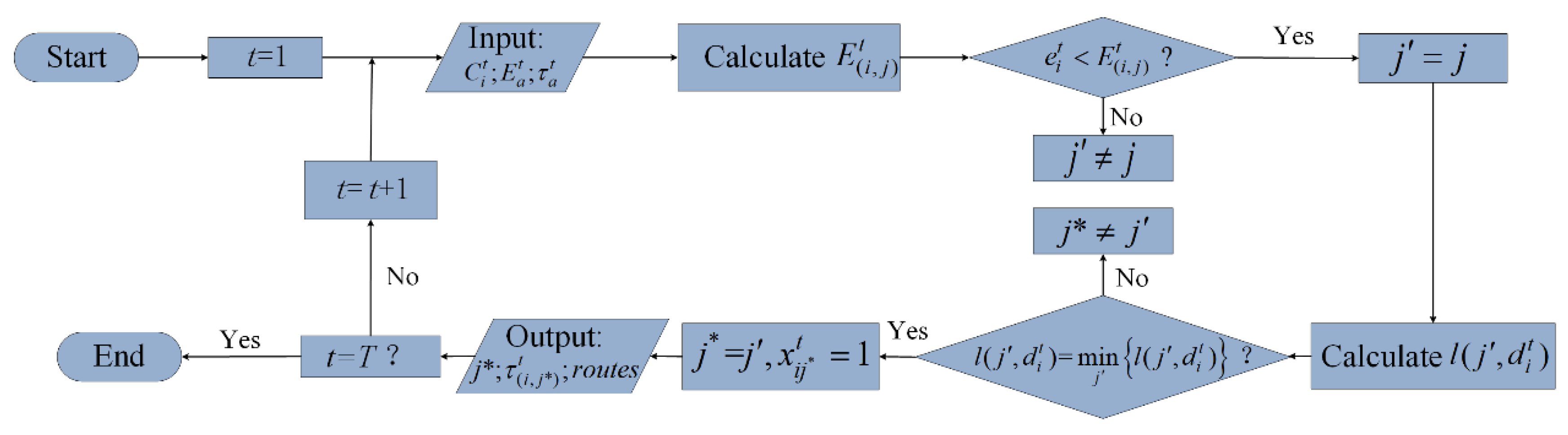
Figure 3 illustrates the flowchart of the CSB strategy.
4.3. Route Guidance Strategy Based on the Travel Cost of Individual Drivers
EV drivers are the decision-makers for travel activities and the service objectives of smart charging services. Therefore, the travel demands of EV drivers should be considered when planning the selection strategy of charging stations. On the premise of charging station reachability, EV drivers often want to reduce their travel cost as much as possible. Travel cost is generally regarded as the optimization criterion for choosing travel routes [50,51]. Travel cost minimization is one of the critical factors for travel demands. Travel cost has multidimensional components during an EV trip, such as travel time, energy consumption, and charging cost [20]. The driving time and energy consumption are closely correlated with the driving distance, with the former being typically proportional to the driving distance with a constant driving speed and the latter having a significant linear relationship with driving distance [52], as well as a significant influence on charging cost; hence, the charging cost would be affected by the driving distance. The driving distance can be used to reflect the integration of travel cost components. Thus, driving distance is minimized to establish the route guidance strategy based on drivers’ travel demands.
Unlike driving time and energy consumption, driving distance is a static factor in a time-varying road network. Adopting driving distance as a selection criterion can utilize such an advantage and avoid complicated prediction. The driving distance from charging stations to destinations is considered in the route guidance strategy. For the routes from origins to charging stations, we assume that EV drivers prefer to focus on reachability rather than distance as mentioned in Assumption 7. As a matter of fact, the driving distance from origins to charging stations is unable to fully reflect the travel direction consistency between charging stations and destinations, but it could be reflected by the driving distance from charging stations to destinations to a certain extent [53]. Furthermore, such an assumption could reduce computing burden and ensure the feasibility of solution. Thus, the driving distance between origins and charging stations is not involved in the strategy. To simplify the description, the route guidance strategy based on the travel cost of individual drivers is represented by the shortest driving distance (SDD) strategy.
As mentioned above, the SDD strategy aims to identify all reachable charging stations, and it directs EVs to the ones with nearest to their destinations. Similar to the CSB strategy, the output of the SDD strategy also includes heuristic suggested charging stations, corresponding routes, and driving time for all charging demands at every time slot. The operating steps of the SDD strategy are detailed as follows:
- At the beginning of time slot t, the minimum energy consumption between all the nodes with and charging station nodes is calculated on the basis of the information of . The minimum energy consumption between charging demand node i and charging station node j is denoted as , which is recorded along with corresponding routes.
- For each at time slot t, is compared with . If , then charging station j is denoted as reachable charging station . Otherwise, charging station j is regarded as the unreachable one and is then deleted from the candidate charging stations.
- For the reachable charging station of , the driving distance between and the node with charging station is calculated. The results are denoted as .
- For each , the driving distance between and reachable charging station is compared. denotes the node with the heuristic suggested charging station. The minimum driving distance between and heuristic suggested charging station needs to satisfy the following condition:The values of decision variable can be determined on the basis of Equation (6). If multiple charging stations with the same and minimum driving distance exist between them and , then one is randomly selected as the heuristic suggested charging station for .
- The driving time on the minimum energy routes between nodes with and corresponding heuristic suggested charging station nodes j* is calculated and recorded. The results are denoted as .
- Before the end of time slot t, the heuristic suggested charging stations j*, driving time , and corresponding routes for the charging demand are output.
The flowchart of the SDD strategy is given in Figure 4.
5. Simulation Analysis
5.1. Scenario Description
The simulation examples for a time-varying road network are designed to explore the performance of the SDD and CSB strategies. The structure of the road network is designed based on the Sioux Falls network, which is often adopted to simulate travel optimization problems [54,55,56]. The network consists of 24 nodes and 76 links, as shown in Figure 5. The road network comprises eight nodes with charging stations, which are marked as CS 1 to CS 8. The other nodes, numbered 1–16, are the normal ones without charging stations, which may generate charging demands in every time slot.
Each charging station node in the road network has parameter to reflect the charging levels of the charging station, where j = {1,2,…,7,8}. For the normal nodes, each one has parameter to reflect the stochastic characteristic of charging demand generation, where I = {1,2,…,15,16}. Table A1 and Table A2 (Appendix A) list the values of and , respectively. The simulation example assumes that the initial number of EVs at each charging station is equal to zero, that is, , for each charging station j in the road network.
The information for each charging demand includes the travel destination and remaining energy , which are randomly generated in the simulation example. In every time slot, the travel destination is randomly selected from other normal nodes in the road network if a charging demand occurs in a specific normal node. Moreover, the remaining energy varies within a given interval, and we suppose that its value ranges from 7.2 kWh to 16.8 kWh by referring to the battery capacity of EVs. In general, EVs with a 24-kWh battery are widely used in unban transportation systems [33]. The energy consumption on each link in a time-varying road network varies as time slot passes. The simulation example randomly determines parameter from given intervals for link a at time slot t to reflect such a characteristic. The value intervals of the energy consumption on each link a are listed in Table A3 (Appendix A).
Similar to the energy consumption , the driving time on each link a also has a time-varying characteristic. Similar to parameter , the values of parameter in every time slot are randomly determined based on given intervals for each link a. The value intervals of driving time on each link a are listed in Table A4 (Appendix A). The number of time slots represents the driving time on each link given that the time is slotted into the time slots with identical duration. Without loss of generality, the duration for each time slot is not constrained in the simulation example. In the real-world situation, the duration for time slots could be valued according to actual requirements.
Table A5 (Appendix A) lists the length of each link a, which is denoted by la (km), in the road network. Considering the structure characteristic of road networks, the links with a symmetric relation have the same length.
5.2. Simulation Results and Analysis
On the basis of the example scenario, the SDD and CSB strategies are applied in the route guidance problem with stochastic charging demands in a time-varying road network. The total number of time slots is set as T = 102, T = 103, T = 104, T = 105, and T = 106 to analyze the performance during different time horizons. The SDD and CSB strategies can ensure the reachability of selected charging stations for the charging demands in every time slot, as mentioned in Section 4. The charging demands of EV drivers can be satisfied by both strategies. Therefore, the simulation example focuses on the effects of the proposed strategies on the operation efficiency of charging stations. The number of EVs in a charging station is a critical factor that reflects the operation state of the charging station. Figure 6 presents the average number of EVs at each charging station during different time horizons T under the proposed strategies, which is computed by averaging over all time slots over the entire number of EVs.
In Figure 6, cases (a)–(h) respectively show the average number of EVs in CS 1–CS 8 during different time horizons. The change trends of the average EV number during different time horizons reflect the stability of charging stations under specific scenarios. Stability is an important criterion for guaranteeing the operation efficiency of charging stations. If the average number of EVs in a charging station has a flat change trend as the time horizon increases, then the charging station would operate stably for the given scenarios [57]; otherwise, the average number of EVs in the charging station would increase rapidly as the time horizon increases. The figure depicts that the SDD and CSB strategies can stabilize the operation states for CS 1–CS 8 under the example scenario, because the number of EVs in all charging stations has flat change trends as time horizon T varies. Although fluctuation trends exist when the time horizon ranges from T = 102 to T = 104 for several charging stations under specific strategies, such as CS 2 under the SDD strategy, CS 3 under the CSB strategy, and CS 5 under both strategies, all charging stations could reach a stable state after the time horizon T = 104. A comparison of the average EV number in CS 1–CS 8 with a stable state shows a difference between the SDD and CSB strategies. For the SDD strategy, the average number of EVs in CS 5 is greater than that in other charging stations because the vehicle balance of charging stations is not considered. The average EV number under the CSB strategy has a similar trend in all charging stations.
Although the average EV number is a critical reflection of the stability of each charging station, it cannot perfectly represent the actual number of EVs in every time slot. The EV number in charging stations at different time slots may vary during the time horizon. As time slots pass, there exists the obvious difference between the maximum and minimum numbers of EVs in a charging station. If the EV number in a selected charging station is relatively large, then the drivers would be reluctant to charge their vehicles by using it at the corresponding time slot. This condition would negatively influence the implementation efficiency of the route guidance service. Therefore, during the time horizon T, the maximum number of EVs at each charging station is often regarded as the bottleneck in the application of route guidance strategies under real-world situations. Figure 7 presents the maximum number of EVs at each charging station during different time horizons T based on the simulation example to compare the performances of the SDD and CSB strategies.
The maximum number of EVs at each charging station under the SDD and CSB strategies is depicted in Figure 7, where cases (a)–(e) illustrate the results during different time horizons, ranging from T = 102 to T = 106, respectively. In case (a), the maximum number of EVs in CS 1–CS 8 under the SDD strategy is less than that under the CSB strategy. However, when the time horizon T = 103, as shown in case (b), the EV number in CS 5 under the SDD strategy is larger than that under the CSB strategy. In case (c), the SDD strategy enlarges the maximum number of EVs in most charging stations, especially in CS 5, compared with case (b). The extreme gap of maximum EV number among the charging stations is equal to 32. By contrast, the maximum number of EVs under the CSB strategy has a moderate degree of change for all charging stations. The maximum number of EVs in CS 3 and CS 5 in particular has a decreasing trend unlike case (b). The extreme gap of maximum EV number among the charging stations is equal to 7. When the time horizon T = 104, as shown in case (d), the maximum number of EVs under the SDD strategy increases for all charging stations, and the maximum EV number in CS 5 and CS 7 is larger than that under the CSB strategy. The extreme gap in the maximum EV number among the charging stations under the SDD and CSB strategies is equal to 41 and 7, respectively, thereby indicating a visible difference in vehicle balance among different charging stations between the two strategies. In case (e), the maximum EV number in CS 5, CS 6, and CS 7 under the SDD strategy is larger than that under the CSB strategy. The extreme gap of maximum EV number among the charging stations reaches 48 under the SDD strategy. By contrast, the maximum number of EVs presents a balanced state for different charging stations under the CSB strategy. The extreme gap of maximum EV number among the charging stations is equal to 7.
A comparison of the performances of the SDD and CSB strategies based on the simulation example shows that the CSB strategy has an advantage in vehicle balance among different charging stations, especially in the situation with a long time horizon. Thus, using the CSB strategy would avoid the negative influence of the large number of EVs in a charging station. Unlike the CSB strategy, the SDD strategy would enlarge the gap of the number of EVs at different charging stations as the time horizon increases, thereby affecting the operation efficiency of the charging stations that have relatively more vehicles. However, in the situation with a short time horizon, the SDD strategy, which considers the travel cost of EV drivers, could address stochastic charging demands because of the unobvious difference in the performance of the two strategies in such a situation. In summary, the CSB strategy is suitable to be applied in long-term transportation scenario due to its ability to stabilize the charging service system. By contrast, the SDD strategy fits the short-term transportation scenario to reduce the travel cost of individual drivers.
5.3. Parameter Analysis for Scenario Characteristics
When discussing the route guidance problem for stochastic charging demands, in addition to time horizon, the scenario characteristics have significant effects on the performance of the proposed strategies. For problem formulation, parameter λi and μj are used to present the stochastic characteristics of charging demands and processes, respectively, as mentioned in Section 3. Such parameters can also reflect the scenario characteristics in terms of the EV scale and charging level. For instance, a large parameter λi represents a large EV scale in node i. A large parameter μj illustrates a high charging level of the charging station in node j. Parameters λi and μj are set as different values to explore the performance of route guidance strategies under different scenario parameters. The values of parameter λi for all normal nodes i are set as identical value λ to highlight the effects of parameter values on the simulation results. The values of parameter μj for all charging station nodes j are also set as identical value μ. The time horizon is set as T = 106 for all parameter scenarios. Figure 8 presents the maximum number of EVs at each charging station under the SDD strategy as parameters and vary. The value of is set as 0.1, 0.2, 0.3, 0.4, and 0.5. The value of is set as 0.6, 0.7, 0.8, 0.9, and 1.0. A parameter scenario consists of a pair of parameters and . Thus, a total of 25 parameter scenarios are considered.
In Figure 8, cases (a)–(h) respectively illustrate the maximum EV number in CS 1–CS 8 under the SDD strategy for the different parameter scenarios. In several parameter scenarios, the maximum EV number in a specific charging station may exceed its sustainable limit, which indicates that the charging station is unstable. For such a scenario, we let the maximum EV number be equal to zero in the figure. The threshold of sustainable number of EVs for all charging stations is set as 120. In case (a), as parameter increases, the maximum EV number in CS 1 presents a decreasing trend. This phenomenon indicates that the maximum EV number reduces as the charging level of the charging station increases. By contrast, as parameter increases, the maximum number of EVs in CS 1 has an increasing trend, which indicates that the maximum EV number increases as the EV scale increases in the road network. Among all parameter scenarios, the peak and lowest values of the maximum EV number are equal to 2 and 29, respectively. In case (b), as the scenario parameters change, the change trend of the maximum EV number in CS 2 is similar to that in CS 1. However, unlike case (a), unstable parameter scenarios exist in case (b). Among all stable parameter scenarios, the peak and lowest values of the maximum EV number equal 3 and 82, respectively. In cases (c)–(h), the change trend of the maximum number of EVs in CS 3–CS 8 is also similar to that in CS 1. Similar to CS 2, the unstable state would exist in CS 3–CS 8 under specific parameter scenarios. Among all stable parameter scenarios, the lowest values of the maximum EV number in CS 3–CS 8 are all equal to 4. Comparatively, the peak values of the maximum EV number in CS 3–CS8 are respectively equal to 103, 41, 95, 58, 69, and 67. For a transportation system, the charging service is unstable until all charging stations can reach stability. Therefore, if at least one unstable charging station exists in the road network under a parameter scenario, then the SDD strategy cannot be applied in the parameter scenario. The parameter scenarios that cannot support the SDD strategy can be determined based on such a criterion. The parameter pairs of the unstable scenarios include , , , , , , ,, , , and . For all the stable parameter scenarios in each case, a significant change trend can be observed as the parameters vary, which indicates that the SDD strategy is sensitive to the change in scenarios.
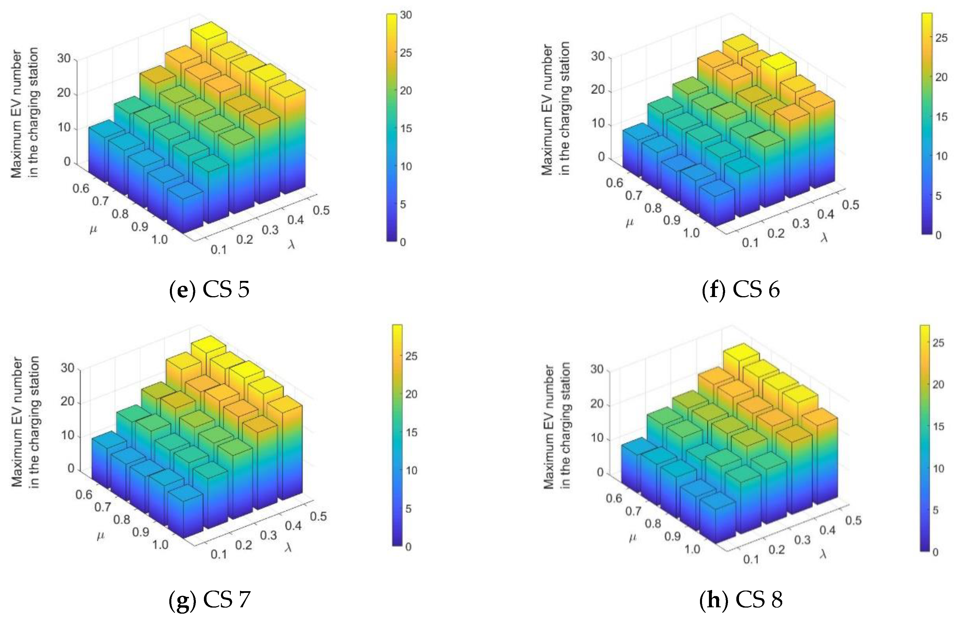
On the basis of the parameter scenarios and the time horizon mentioned above, the CSB strategy is further applied in the route guidance problem with stochastic charging demands. As parameters and vary, the maximum EV number at each charging station is obtained, as shown in Figure 9.
In Figure 9, cases (a)–(h) respectively present the maximum number of EVs in CS 1–CS 8 under the CSB strategies for the different parameter scenarios. In case (a), the maximum number of EVs in CS 1 broadly presents a flat increasing trend as parameter μ decreases and parameter λ increases. For several individual scenarios, a moderate fluctuation occurs as the parameters vary. The results indicate that a change in scenarios has relatively limited effects on the CSB strategy compared with that on the SDD strategy. Among all parameter scenarios, the peak and lowest values of the maximum EV number in CS 1 are equal to 7 and 20, respectively. In cases (b)–(h), the maximum number of EVs in CS 2–CS 8 shows a similar change trend to that in CS 1. Among all parameter scenarios, the lowest values of the maximum EV number in CS 2–CS 8 are respectively equal to 9, 10, 11, 10, 9, 11, and 10. Comparatively, the peak values of the maximum EV number in CS 2–CS 8 are equal to 26, 30, 32, 30, 28, 29, and 27, respectively. Unlike the SDD strategy, the CSB strategy can stabilize the state of CS 1–CS 8 for all parameter scenarios, thus indicating its advantage in charging station stability.
A comparison of the simulation results in Figure 8 and Figure 9 indicates that, for the SDD and CSB strategies, the maximum EV number increases as parameter decreases and parameter increases, with different change trends. Given the implication of parameters and , the simulation results conform to the operation state of charging stations in real-world situations.
6. Conclusions
In this study, a route guidance problem was formulated by combining the time-varying road network and stochastic charging demands. To address the problem, we proposed two heuristic-based route guidance strategies from two different perspectives, namely, the SDD and CSB strategies. The SDD strategy uses the driving distance as the optimization criterion based on the travel cost of individual drivers. By contrast, the CSB strategy selects the charging stations with the minimum EV number based on the vehicle balance in charging stations. Despite their differences, both strategies can guarantee the reachability of selected charging stations in a time-varying road network. Simulation experiments were implemented to explore the performances of the SDD and CSB strategies. The results indicate that the CSB strategy has an advantage over the SDD strategy in avoiding the negative influence of mass EV charging on the charging station operation, especially in the situation with a relatively long time horizon.
Furthermore, the parameter analysis was carried out through changing the scenario parameters in the simulation experiments. The results present the different performances of SDD and CSB strategies as parameter scenarios vary. For the SDD strategy, the maximum EV number at different charging stations had a significant gap and ranged from approximately 30 to 100. By contrast, for the CSB strategy, the maximum EV number at different charging station exhibited a moderate degree of change and mainly ranged from 25 to 30. Moreover, the SDD strategy may be unable to stabilize the charging service system in some heavily loaded scenarios (i.e., low and high ), but the CSB strategy can stabilize the charging service system for all parameter scenarios. However, if the charging service is in lightly loaded scenarios (i.e., high and low ), the SDD strategy could be employed due to its similar effects on charging stations with the CSB strategy and consideration of the travel cost of individual drivers.
Each normal node is assumed to generate at most one charging demand in every time slot to simplify the problem formulation. Such an assumption is reasonable if each time slot has a relatively short duration. However, as the scale of EVs increases in the urban transportation system, multiple charging demands may occur simultaneously in the same location on road networks, thereby significantly complicating the solving processes for the stochastic charging demands. On the basis of the proposed strategies, a distribution rule regarding the number of charging demand occurrence will be further explored in future work and considered to improve the route guidance strategies. Furthermore, other evaluation metrics, such as waiting time, trip length extension, and energy efficiency, will be introduced in a future study.
Author Contributions
Conceptualization, Y.W. and J.B.; methodology, Y.W.; validation, Y.W. and C.L.; writing, Y.W.; visualization, Y.W., C.L., and C.D.; supervision, J.B., C.L., and C.D.; funding acquisition, J.B. All authors have read and agreed to the published version of the manuscript.
Funding
This work was funded by the National Natural Science Foundation of China (Nos. 71961137008 and 71621001).
Acknowledgments
The authors gratefully acknowledge fruitful discussions with Prof. Bin Li in the University of Rhode Island, as well as financial support from the China Scholarship Council.
Conflicts of Interest
The authors declare no conflict of interest.
Appendix A

Table A1.
Value of parameter for each charging station node.
| Charging station | Charging Station | Charging Station | |||
|---|---|---|---|---|---|
| CS 1 | 0.74 | CS 4 | 0.90 | CS 7 | 0.94 |
| CS 2 | 0.84 | CS 5 | 0.78 | CS 8 | 0.90 |
| CS 3 | 0.94 | CS 6 | 0.87 |
Table A2.
Value of parameter for each normal node.
| Normal Node | Normal Node | Normal Node | Normal Node | ||||
|---|---|---|---|---|---|---|---|
| 1 | 0.31 | 5 | 0.20 | 9 | 0.18 | 13 | 0.57 |
| 2 | 0.62 | 6 | 0.13 | 10 | 0.27 | 14 | 0.35 |
| 3 | 0.32 | 7 | 0.50 | 11 | 0.15 | 15 | 0.52 |
| 4 | 0.69 | 8 | 0.25 | 12 | 0.26 | 16 | 0.67 |
Table A3.
Value intervals of energy consumption for link a at time slot t.
| Link a | Link a | Link a | |||
|---|---|---|---|---|---|
| 1–CS 1 | (2.64, 5.76) | 9–7 | (2.16, 4.8) | CS 1–2 | (1.68, 4.08) |
| 1–4 | (3.6, 5.04) | 9–11 | (2.16, 5.04) | CS 2–3 | (3.6, 6.96) |
| 2–CS 1 | (2.4, 4.8) | 10–CS 4 | (2.64, 5.52) | CS 2–4 | (2.88, 6.48) |
| 2–3 | (1.92, 4.56) | 10–12 | (1.44, 4.08) | CS 2–5 | (3.6, 4.8) |
| 3–2 | (3.12, 4.32) | 10–CS 7 | (2.64, 4.56) | CS 3–2 | (2.88, 6) |
| 3–CS 4 | (1.44, 3.84) | 11–9 | (2.16, 3.6) | CS 3–CS 4 | (2.88, 5.28) |
| 3–CS 2 | (1.2, 4.32) | 11–CS 7 | (1.2, 4.56) | CS 3–14 | (2.16, 4.8) |
| 4–1 | (2.16, 3.6) | 11–16 | (1.44, 3.36) | CS 4–3 | (1.2, 4.8) |
| 4–CS 2 | (2.4, 5.28) | 12–10 | (2.16, 4.8) | CS 4–7 | (2.64, 6) |
| 4–6 | (3.12, 6.48) | 12–13 | (2.4, 4.8) | CS 4–10 | (3.12, 6.72) |
| 5–CS 2 | (2.88, 5.28) | 12–CS 8 | (1.92, 4.8) | CS 4–CS 3 | (2.88, 4.8) |
| 5–6 | (2.4, 3.6) | 13–CS 7 | (3.36, 5.04) | CS 5–6 | (1.2, 3.12) |
| 5–7 | (1.68, 3.6) | 13–12 | (2.64, 4.56) | CS 5–7 | (1.44, 3.36) |
| 6–4 | (1.44.5.04) | 13–15 | (1.68, 4.56) | CS 5–8 | (3.12, 5.04) |
| 6–5 | (2.16, 3.6) | 13–16 | (1.44, 5.04) | CS 5–9 | (2.4, 5.04) |
| 6–CS 5 | (2.16, 5.28) | 14–CS 3 | (3.12, 5.04) | CS 6–6 | (2.16, 4.08) |
| 6–CS 6 | (3.6, 5.52) | 14–CS 8 | (2.88, 6.24) | CS 6–8 | (1.92, 5.52) |
| 7–5 | (3.6, 5.52) | 15–13 | (1.92, 5.28) | CS 7–7 | (1.68, 4.56) |
| 7–CS 4 | (1.92, 4.32) | 15–CS 8 | (1.2, 4.56) | CS 7–10 | (3.6, 6.72) |
| 7–CS 7 | (3.36, 5.52) | 15–16 | (2.16, 5.28) | CS 7–11 | (2.16, 3.84) |
| 7–9 | (2.64, 6.24) | 16–8 | (2.4, 4.08) | CS 7–13 | (1.44, 2.88) |
| 7–CS 5 | (2.4, 4.32) | 16–11 | (2.4, 6) | CS 8–12 | (2.4, 3.6) |
| 8–CS 6 | (3.36, 4.8) | 16–13 | (3.36, 6.72) | CS 8–14 | (1.2, 3.84) |
| 8–CS 5 | (3.12, 4.8) | 16–15 | (3.6, 6.96) | CS 8–15 | (2.64, 5.28) |
| 8–16 | (2.4, 3.84) | CS 1–1 | (2.16, 5.28) | 2–CS 3 | (2.16, 4.32) |
| 9–CS 5 | (1.2, 4.32) |
Table A4.
Value intervals of driving time for link a at time slot t.
| Link a | Link a | Link a | |||
|---|---|---|---|---|---|
| 1–CS 1 | (2, 5) | 9–7 | (1, 2) | CS 1–2 | (1, 3) |
| 1–4 | (1, 4) | 9–11 | (1, 2) | CS 2–3 | (1, 2) |
| 2–CS 1 | (2, 3) | 10–CS 4 | (1, 2) | CS 2–4 | (2, 4) |
| 2–3 | (1, 2) | 10–12 | (1, 2) | CS 2–5 | (1, 3) |
| 3–2 | (2, 3) | 10–CS 7 | (2, 4) | CS 3–2 | (1, 2) |
| 3–CS 4 | (2, 3) | 11–9 | (1, 2) | CS 3–CS 4 | (1, 3) |
| 3–CS 2 | (1, 4) | 11–CS 7 | (2, 4) | CS 3–14 | (1, 2) |
| 4–1 | (1, 2) | 11–16 | (1, 2) | CS 4–3 | (1, 2) |
| 4–CS 2 | (2, 4) | 12–10 | (2, 3) | CS 4–7 | (1, 3) |
| 4–6 | (1, 2) | 12–13 | (1, 2) | CS 4–10 | (1, 3) |
| 5–CS 2 | (1, 2) | 12–CS 8 | (1, 4) | CS 4–CS 3 | (1, 2) |
| 5–6 | (1, 2) | 13–CS 7 | (1, 3) | CS 5–6 | (1, 2) |
| 5–7 | (2, 3) | 13–12 | (1, 2) | CS 5–7 | (1, 2) |
| 6–4 | (1, 2) | 13–15 | (2, 3) | CS 5–8 | (1, 2) |
| 6–5 | (1, 2) | 13–16 | (1, 2) | CS 5–9 | (1, 2) |
| 6–CS 5 | (1, 3) | 14–CS 3 | (2, 4) | CS 6–6 | (1, 3) |
| 6–CS 6 | (1, 2) | 14–CS 8 | (2, 3) | CS 6–8 | (2, 3) |
| 7–5 | (1, 2) | 15–13 | (2, 3) | CS 7–7 | (1, 3) |
| 7–CS 4 | (2, 5) | 15–CS 8 | (2, 5) | CS 7–10 | (1, 3) |
| 7–CS 7 | (2, 4) | 15–16 | (1, 2) | CS 7–11 | (1, 2) |
| 7–9 | (1, 2) | 16–8 | (1, 3) | CS 7–13 | (1, 2) |
| 7–CS 5 | (1, 3) | 16–11 | (1, 2) | CS 8–12 | (2, 3) |
| 8–CS 6 | (2, 5) | 16–13 | (1, 3) | CS 8–14 | (1, 2) |
| 8–CS 5 | (2, 4) | 16–15 | (2, 3) | CS 8–15 | (1, 2) |
| 8–16 | (1, 2) | CS 1–1 | (1, 2) | 2–CS 3 | (1, 3) |
| 9–CS 5 | (2, 3) |
Table A5.
Length of link a in the road network.
| Link a | la (km) | Link a | la (km) | Link a | la (km) |
|---|---|---|---|---|---|
| 1–CS 1 | 23 | 9–7 | 15 | CS 1–2 | 11 |
| 1–4 | 12 | 9–11 | 10 | CS 2–3 | 10 |
| 2–CS 1 | 11 | 10–CS 4 | 14 | CS 2–4 | 10 |
| 2–3 | 10 | 10–12 | 11 | CS 2–5 | 11 |
| 3–2 | 10 | 10–CS 7 | 12 | CS 3–2 | 17 |
| 3–CS 4 | 20 | 11–9 | 10 | CS 3–CS 4 | 12 |
| 3–CS 2 | 10 | 11–CS 7 | 12 | CS 3–14 | 22 |
| 4–1 | 12 | 11–16 | 16 | CS 4–3 | 20 |
| 4–CS 2 | 10 | 12–10 | 11 | CS 4–7 | 10 |
| 4–6 | 12 | 12–13 | 12 | CS 4–10 | 14 |
| 5–CS 2 | 11 | 12–CS 8 | 10 | CS 4–CS 3 | 12 |
| 5–6 | 10 | 13–CS 7 | 11 | CS 5–6 | 11 |
| 5–7 | 12 | 13–12 | 12 | CS 5–7 | 11 |
| 6–4 | 12 | 13–15 | 10 | CS 5–8 | 10 |
| 6–5 | 10 | 13–16 | 16 | CS 5–9 | 11 |
| 6–CS 5 | 11 | 14–CS 3 | 22 | CS 6–6 | 12 |
| 6–CS 6 | 12 | 14–CS 8 | 12 | CS 6–8 | 12 |
| 7–5 | 12 | 15–13 | 10 | CS 7–7 | 18 |
| 7–CS 4 | 10 | 15–CS 8 | 11 | CS 7–10 | 12 |
| 7–CS 7 | 18 | 15–16 | 10 | CS 7–11 | 12 |
| 7–9 | 15 | 16–8 | 30 | CS 7–13 | 11 |
| 7–CS 5 | 11 | 16–11 | 16 | CS 8–12 | 10 |
| 8–CS 6 | 12 | 16–13 | 16 | CS 8–14 | 12 |
| 8–CS 5 | 10 | 16–15 | 10 | CS 8–15 | 11 |
| 8–16 | 30 | CS 1–1 | 23 | 2–CS 3 | 17 |
| 9–CS 5 | 11 |
References
- International Energy Agency. Global EV Outlook 2017; IEA: Paris, France, 2017. [Google Scholar]
- Rezvani, Z.; Jansson, J.; Bodin, J. Advances in consumer electric vehicle adoption research: A review and research agenda. Transp. Res. Part D Transp. Environ. 2015, 34, 122–136. [Google Scholar] [CrossRef] [Green Version]
- Melliger, M.; Van Vliet, O.; Liimatainen, H. Anxiety vs. reality—Sufficiency of battery electric vehicle range in Switzerland and Finland. Transp. Res. Part D Transp. Environ. 2018, 65, 101–115. [Google Scholar] [CrossRef]
- Wang, Y.; Bi, J.; Zhao, X.; Guan, W. A geometry-based algorithm to provide guidance for electric vehicle charging. Transp. Res. Part D Transp. Environ. 2018, 63, 890–906. [Google Scholar] [CrossRef]
- Gendreau, M.; Ghiani, G.; Guerriero, E. Time-dependent routing problems: A review. Comput. Oper. Res. 2015, 64, 189–197. [Google Scholar] [CrossRef]
- Artmeier, A.; Haselmayr, J.; Leucker, M.; Sachenbacher, M. The shortest path problem revisited: Optimal routing for electric vehicles. In Annual Conference on Artificial Intelligence; Springer: Berlin/Heidelberg, Germany, 2010; pp. 309–316. [Google Scholar]
- Storandt, S. Quick and energy-efficient routes: Computing constrained shortest paths for electric vehicles. In Proceedings of the 5th ACM SIGSPATIAL International Workshop on Computational Transportation Science, Redondo Beach, CA, USA, 7–9 November 2012; ACM: New York, NY, USA, 2012; pp. 20–25. [Google Scholar]
- Neaimeh, M.; Hill, G.; Hübner, Y.; Blythe, P.T. Routing systems to extend the driving range of electric vehicles. IET Intell. Transp. Syst. 2013, 7, 327–336. [Google Scholar] [CrossRef] [Green Version]
- Sweda, T.; Dolinskaya, I.; Klabjan, D. Adaptive routing and recharging policies for electric vehicles. Transp. Sci. 2017, 51, 1326–1348. [Google Scholar] [CrossRef]
- Qin, H.; Zhang, W. Charging scheduling with minimal waiting in a network of electric vehicles and charging stations. In Proceedings of the Eighth ACM International Workshop on Vehicular Inter-Networking, Las Vegas, NV, USA, 19 –23 September 2011; ACM: New York, NY, USA, 2011; pp. 51–60. [Google Scholar]
- Said, D.; Cherkaoui, S.; Khoukhi, L. Queuing model for EVs charging at public supply stations. In Proceedings of the 2013 9th International Wireless Communications and Mobile Computing Conference (IWCMC), Sardinia, Italy, 1–5 July 2013; IEEE: Piscataway, NJ, USA, 2013; pp. 65–70. [Google Scholar]
- Yang, S.; Cheng, W.; Hsu, Y.; Gan, C.; Lin, Y. Charge scheduling of electric vehicles in highways. Math. Comput. Model. 2013, 57, 2873–2882. [Google Scholar] [CrossRef]
- De Weerdt, M.; Stein, S.; Gerding, E.; Robu, V.; Jennings, N. Intention-aware routing of electric vehicles. IEEE Trans. Intell. Transp. Syst. 2015, 17, 1472–1482. [Google Scholar] [CrossRef] [Green Version]
- Zhang, Y.; Aliya, B.; Zhou, Y.; You, I.; Zhang, X.; Pau, G.; Collotta, M. Shortest feasible paths with partial charging for battery-powered electric vehicles in smart cities. Pervasive Mob. Comput. 2018, 50, 82–93. [Google Scholar] [CrossRef]
- Wang, T.; Cassandras, C.; Pourazarm, S. Energy-aware vehicle routing in networks with charging nodes. IFAC Proc. Vol. 2014, 47, 9611–9616. [Google Scholar] [CrossRef] [Green Version]
- Cao, Y.; Tang, S.; Li, C.; Zhang, P.; Tan, Y.; Zhang, Z.; Li, J. An optimized EV charging model considering TOU price and SOC curve. IEEE Trans. Smart Grid 2011, 3, 388–393. [Google Scholar] [CrossRef]
- Liu, C.; Wu, J.; Long, C. Joint charging and routing optimization for electric vehicle navigation systems. IFAC Proc. Vol. 2014, 47, 2106–2111. [Google Scholar] [CrossRef] [Green Version]
- Yagcitekin, B.; Uzunoglu, M. A double-layer smart charging strategy of electric vehicles taking routing and charge scheduling into account. Appl. Energy 2016, 167, 407–419. [Google Scholar] [CrossRef]
- Sun, Z.; Zhou, X. To save money or to save time: Intelligent routing design for plug-in hybrid electric vehicle. Transp. Res. Part D Transp. Environ. 2016, 43, 238–250. [Google Scholar] [CrossRef]
- Wang, Y.; Bi, J.; Guan, W.; Zhao, X. Optimising route choices for the travelling and charging of battery electric vehicles by considering multiple objectives. Transp. Res. Part D Transp. Environ. 2018, 64, 246–261. [Google Scholar] [CrossRef]
- Wang, Y.; Jiang, J.; Mu, T. Context-aware and energy-driven route optimization for fully electric vehicles via crowdsourcing. IEEE Trans. Intell. Transp. Syst. 2013, 14, 1331–1345. [Google Scholar] [CrossRef]
- Abousleiman, R.; Rawashdeh, O.; Abousleiman, R.; Rawashdeh, O. A Bellman-Ford approach to energy efficient routing of electric vehicles. In Proceedings of the 2015 IEEE Transportation Electrification Conference and Expo (ITEC), Dearborn, MI, USA, 14–17 June 2015; IEEE: Piscataway, NJ, USA, 2015; pp. 1–4. [Google Scholar]
- Strehler, M.; Merting, S.; Schwan, C. Energy-efficient shortest routes for electric and hybrid vehicles. Transp. Res. Part B Methodol. 2017, 103, 111–135. [Google Scholar] [CrossRef]
- Fiori, C.; Ahn, K.; Rakha, H. Optimum routing of battery electric vehicles: Insights using empirical data and microsimulation. Transp. Res. Part D Transp. Environ. 2018, 64, 262–272. [Google Scholar] [CrossRef]
- Fernández, R. A more realistic approach to electric vehicle contribution to greenhouse gas emissions in the city. J. Clean. Prod. 2018, 172, 949–959. [Google Scholar] [CrossRef]
- Alizadeh, M.; Wai, H.; Scaglione, A.; Goldsmith, A.; Fan, Y.; Javidi, T. Optimized path planning for electric vehicle routing and charging. In Proceedings of the 2014 52nd Annual Allerton Conference on Communication, Control, and Computing (Allerton), Monticello, IL, USA, 30 September–3 October 2014; IEEE: Piscataway, NJ, USA, 2014; pp. 25–32. [Google Scholar]
- Yi, Z.; Bauer, P. Optimal stochastic eco-routing solutions for electric vehicles. IEEE Trans. Intell. Transp. Syst. 2018, 19, 3807–3817. [Google Scholar] [CrossRef]
- Zhang, S.; Luo, Y.; Li, K. Multi-objective route search for electric vehicles using ant colony optimization. In Proceedings of the 2016 American Control Conference (ACC), Boston, MA, USA, 6–8 July 2016; IEEE: Piscataway, NJ, USA, 2016; pp. 637–642. [Google Scholar]
- Jafari, E.; Boyles, S. Multicriteria stochastic shortest path problem for electric vehicles. Netw. Spat. Econ. 2017, 17, 1043–1070. [Google Scholar] [CrossRef]
- Daina, N.; Sivakumar, A.; Polak, J. Electric vehicle charging choices: Modelling and implications for smart charging services. Transp. Res. Part C Emerg. Technol. 2017, 81, 36–56. [Google Scholar] [CrossRef]
- Huber, G.; Bogenberger, K. Long-Trip Optimization of Charging Strategies for Battery Electric Vehicles. Transp. Res. Rec. 2015, 2497, 45–53. [Google Scholar] [CrossRef]
- Jiang, N.; Xie, C.; Duthie, J.; Waller, S. A network equilibrium analysis on destination, route and parking choices with mixed gasoline and electric vehicular flows. EURO J. Transp. Logist. 2014, 3, 55–92. [Google Scholar] [CrossRef] [Green Version]
- He, F.; Yin, Y.; Lawphongpanich, S. Network equilibrium models with battery electric vehicles. Transp. Res. Part B Methodol. 2014, 67, 306–319. [Google Scholar] [CrossRef]
- Xie, C.; Jiang, N. Relay requirement and traffic assignment of electric vehicles. Comput. -Aided Civ. Infrastruct. Eng. 2016, 31, 580–598. [Google Scholar] [CrossRef]
- Xu, M.; Meng, Q.; Liu, K. Network user equilibrium problems for the mixed battery electric vehicles and gasoline vehicles subject to battery swapping stations and road grade constraints. Transp. Res. Part B Methodol. 2017, 99, 138–166. [Google Scholar] [CrossRef]
- Hung, Y.; Michailidis, G. Optimal routing for electric vehicle service systems. Eur. J. Oper. Res. 2015, 247, 515–524. [Google Scholar] [CrossRef]
- Bi, J.; Wang, Y.; Sai, Q.; Ding, C. Estimating remaining driving range of battery electric vehicles based on real-world data: A case study of Beijing, China. Energy 2019, 169, 833–843. [Google Scholar] [CrossRef]
- Huang, Y.; Zhao, L.; Van Woensel, T.; Gross, J. Time-dependent vehicle routing problem with path flexibility. Transp. Res. Part B Methodol. 2017, 95, 169–195. [Google Scholar] [CrossRef]
- Neely, M.; Modiano, E.; Rohrs, C. Dynamic power allocation and routing for time-varying wireless networks. IEEE J. Sel. Areas Commun. 2005, 23, 89–103. [Google Scholar] [CrossRef] [Green Version]
- Polson, N.; Sokolov, V. Deep learning for short-term traffic flow prediction. Transp. Res. Part C Emerg. Technol. 2017, 79, 1–17. [Google Scholar] [CrossRef] [Green Version]
- Cheng, L.; Chang, Y.; Huang, R. Mitigating voltage problem in distribution system with distributed solar generation using electric vehicles. IEEE Trans. Sustain. Energy 2015, 6, 1475–1484. [Google Scholar] [CrossRef]
- Xu, Z.; Su, W.; Hu, Z.; Song, Y.; Zhang, H. A hierarchical framework for coordinated charging of plug-in electric vehicles in China. IEEE Trans. Smart Grid 2015, 7, 428–438. [Google Scholar] [CrossRef]
- Esfahani, M.; Yousefi, G. Real time congestion management in power systems considering quasi-dynamic thermal rating and congestion clearing time. IEEE Trans. Ind. Inform. 2016, 12, 745–754. [Google Scholar] [CrossRef]
- Gnann, T.; Funke, S.; Jakobsson, N.; Plötz, P.; Sprei, F.; Bennehag, A. Fast charging infrastructure for electric vehicles: Today’s situation and future needs. Transp. Res. Part D Transp. Environ. 2018, 62, 314–329. [Google Scholar] [CrossRef]
- Li, B.; Eryilmaz, A. Non-derivative algorithm design for efficient routing over unreliable stochastic networks. Perform. Eval. 2014, 71, 44–60. [Google Scholar] [CrossRef]
- Franke, T.; Krems, J.F. Understanding charging behaviour of electric vehicle users. Transp. Res. Part F Traffic Psychol. Behav. 2013, 21, 75–89. [Google Scholar] [CrossRef]
- Raslavičius, L.; Azzopardi, B.; Keršys, A.; Starevičius, M.; Bazaras, Ž.; Makaras, R. Electric vehicles challenges and opportunities: Lithuanian review. Renew. Sustain. Energy Rev. 2015, 42, 786–800. [Google Scholar] [CrossRef]
- Bi, J.; Wang, Y.; Sun, S.; Guan, W. Predicting Charging Time of Battery Electric Vehicles Based on Regression and Time-Series Methods: A Case Study of Beijing. Energies 2018, 11, 1040. [Google Scholar] [CrossRef] [Green Version]
- Fu, L.; Sun, D.; Rilett, L.R. Heuristic shortest path algorithms for transportation applications: State of the art. Comput. Oper. Res. 2006, 33, 3324–3343. [Google Scholar] [CrossRef]
- Gao, S.; Frejinger, E.; Ben-Akiva, M. Adaptive route choices in risky traffic networks: A prospect theory approach. Transp. Res. Part C Emerg. Technol. 2010, 18, 727–740. [Google Scholar] [CrossRef]
- Braekers, K.; Ramaekers, K.; Van Nieuwenhuyse, I. The vehicle routing problem: State of the art classification and review. Comput. Ind. Eng. 2016, 99, 300–313. [Google Scholar] [CrossRef]
- Bi, J.; Wang, Y.; Zhang, J. A data-based model for driving distance estimation of battery electric logistics vehicles. EURASIP J. Wirel. Commun. Netw. 2018, 2018, 251. [Google Scholar] [CrossRef]
- Yang, Y.; Yao, E.; Yang, Z.; Zhang, R. Modeling the charging and route choice behavior of BEV drivers. Transp. Res. Part C Emerg. Technol. 2016, 65, 190–204. [Google Scholar] [CrossRef]
- Meng, Q.; Yang, H. Benefit distribution and equity in road network design. Transp. Res. Part B Methodol. 2002, 36, 19–35. [Google Scholar] [CrossRef]
- Chow, J.; Regan, A. Network-based real option models. Transp. Res. Part B Methodol. 2011, 45, 682–695. [Google Scholar] [CrossRef]
- Bell, M.; Kurauchi, F.; Perera, S.; Wong, W. Investigating transport network vulnerability by capacity weighted spectral analysis. Transp. Res. Part B Methodol. 2017, 99, 251–266. [Google Scholar] [CrossRef]
- Hung, Y.; Michailidis, G. Stability and control of acyclic stochastic processing networks with shared resources. IEEE Trans. Autom. Control 2012, 57, 489–494. [Google Scholar] [CrossRef]
Figure 1.
Reachable and unreachable charging stations (CS).

Figure 2.
Stochastic route guidance problem in a time-varying road network.

Figure 3.
Flowchart of the charging station balance (CSB) strategy.

Figure 4.
Flowchart of the shortest driving distance (SDD) strategy.

Figure 5.
Sioux Falls road network for the simulation example.

Figure 6.
Average electric vehicle (EV) number at each charging station during different time horizons T.
Figure 6.
Average electric vehicle (EV) number at each charging station during different time horizons T.


Figure 7.
Maximum EV number at each charging station during different time horizons T.

Figure 8.
Change trends of the maximum EV number at each charging station under the SDD strategy, where λ is the possibility of charging demand occurrence in normal nodes at each time slot, and μ is the possibility of an EV leaving the charging station after completing charging at each time slot.
Figure 8.
Change trends of the maximum EV number at each charging station under the SDD strategy, where λ is the possibility of charging demand occurrence in normal nodes at each time slot, and μ is the possibility of an EV leaving the charging station after completing charging at each time slot.

Figure 9.
Change trends of the maximum EV number in each charging station under the CSB strategy, where λ is the possibility of charging demand occurrence in normal nodes at each time slot, and μ is the possibility of an EV leaving the charging station after completing charging at each time slot.
Figure 9.
Change trends of the maximum EV number in each charging station under the CSB strategy, where λ is the possibility of charging demand occurrence in normal nodes at each time slot, and μ is the possibility of an EV leaving the charging station after completing charging at each time slot.


© 2020 by the authors. Licensee MDPI, Basel, Switzerland. This article is an open access article distributed under the terms and conditions of the Creative Commons Attribution (CC BY) license (http://creativecommons.org/licenses/by/4.0/).
Share and Cite
MDPI and ACS Style
Wang, Y.; Bi, J.; Lu, C.; Ding, C. Route Guidance Strategies for Electric Vehicles by Considering Stochastic Charging Demands in a Time-Varying Road Network. Energies 2020, 13, 2287. https://0-doi-org.brum.beds.ac.uk/10.3390/en13092287
AMA Style
Wang Y, Bi J, Lu C, Ding C. Route Guidance Strategies for Electric Vehicles by Considering Stochastic Charging Demands in a Time-Varying Road Network. Energies. 2020; 13(9):2287. https://0-doi-org.brum.beds.ac.uk/10.3390/en13092287
Chicago/Turabian StyleWang, Yongxing, Jun Bi, Chaoru Lu, and Cong Ding. 2020. "Route Guidance Strategies for Electric Vehicles by Considering Stochastic Charging Demands in a Time-Varying Road Network" Energies 13, no. 9: 2287. https://0-doi-org.brum.beds.ac.uk/10.3390/en13092287
Note that from the first issue of 2016, this journal uses article numbers instead of page numbers. See further details here.