A Supervisory Control Strategy for Improving Energy Efficiency of Artificial Lighting Systems in Greenhouses


1
Politecnico di Torino, Corso Duca degli Abruzzi, 24, 10129 Torino, Italy
2
Andlinger Center for Energy and The Environment, Princeton University, Olden St., 86, Princeton, NJ 08540, USA
3
Freelance Innovation Consultant, 12100 Cuneo, Italy
*
Author to whom correspondence should be addressed.
Energies 2021, 14(1), 202; https://0-doi-org.brum.beds.ac.uk/10.3390/en14010202
Submission received: 3 December 2020
/
Revised: 27 December 2020
/
Accepted: 28 December 2020
/
Published: 2 January 2021
(This article belongs to the Special Issue Energy Performance and Indoor Climate in Buildings)
Abstract
:Artificial lighting systems are used in commercial greenhouses to ensure year-round yields. Current Light Emitting Diode (LED) technologies improved the system efficiency. Nevertheless, having artificial lighting systems extended for hectares with power densities over causes energy and power demand of greenhouses to be really significant. The present paper introduces an innovative supervisory and predictive control strategy to optimize the energy performance of the artificial lights of greenhouses. The controller has been implemented in a multi-span plastic greenhouse located in North Italy. The proposed control strategy has been tested on a greenhouse of 1 hectare with a lighting system with a nominal power density of 50 requiring an overall power supply of 1 for a period of 80 days. The results have been compared with the data coming from another greenhouse of 1 hectare in the same conditions implementing a state-of-the-art strategy for artificial lighting control. Results outlines that potential 19.4% cost savings are achievable. Moreover, the algorithm can be used to transform the greenhouse in a viable source of energy flexibility for grid reliability.
1. Introduction
1.1. Energy Consumption of Greenhouses
Commercial greenhouses are facilities used to produce flowers or vegetables throughout the year, leading to higher yields at the same area of land. For this reason, commercial greenhouses are considered an effective method for satisfying the increasing needs of the growing world’s population [1]. However, the energy consumption of those facilities is increased by the necessity of maintaining appropriate indoor environmental conditions to ensure the crop growth (i.e., temperature, humidity, lighting, carbon dioxide concentration should be maintained constantly in certain ranges). Several studies have been focused on assessing the environmental impact of this action [2,3] or reducing the energy consumption related to the commercial greenhouse indoor climate control [4]. Basically, a commercial greenhouse can benefit by the increase in the light input, the reduction of heat losses during cold weather, and the increase in heat removal during the warm season [5]. For these purposes, the scientific literature provides a wide selection of studies focusing on the improvement of the performance of either the envelope [6,7] or the Heating Ventilating and Air Conditioning (HVAC) system [8] or the energy supply [9,10].
Serale et al. showed how nowadays improved control strategies are an alternative cost effective solution that can significantly improve the building energy performance [11,12,13,14]. Commercial greenhouses are not far behind other buildings’ end-uses. Indeed, innovative controllers largely proven to be an effective method to reduce energy consumption or increase crop production of commercial greenhouses. This is particularly true, thanks to the current large amount of data also readily available in those environments [15]. For instance, Van Straten et al. [16] extended the pioneering work of Reference [17,18], investigating a receding horizon optimal control strategy to improve the thermal management of a multi-span greenhouse. Simulation results showed a potential reduction of the energy demand of approximately and an increase of the biomass production of approximately . In Reference [19], the author proposed the use of different optimization algorithms combined with prediction of the greenhouse energy consumption to obtain a significant improvement of energy performance. References [20,21] proposed fuzzy-logic control systems to enhance ventilation, heating, humidifying, and dehumidifying purposes and integrated photoVoltaic (PV) power into commercial greenhouses. Tang et al., in Reference [22], proposed a system that coupled Light Emitting Diode (LED) artificial lights with fiber optic sunlight collectors for a multi-layer cultivation. The system was capable of accelerating vegetables growth rate and reducing the energy consumption of the artificial lighting systems, also thanks to a remote control system. Model-based controllers proved to be particularly effective. For example, Ma et al. [23] verified experimentally a novel simulation model that was able to enhance the performance of a conveyor system used to maintain an optimal micro-climate in the crop boundary layer. References [24,25] adopted Model Predictive Control (MPC) formulation to reduce water and energy consumption and track the set-point of the indoor air temperature. Similarly, Xu et al. have conducted extensive studies investigating the opportunities offered by a model-based receding horizon control approach to enhance profitability of commercial greenhouses [26,27,28]. In particular, they simulated the benefits achievable by means of a two time-scale receding horizon control exploiting short- and long-term weather predictions. In Ref. [28], they focused on the control of the greenhouse’ artificial lighting system, showing that an improved LED can boost the profit margin up to . Finally, Bersani et al. reviewed many other solutions based on MPC that, starting from the acquired data from the the greenhouse, were able to enhance energy management strategies, allowing a sensible reduction in energy consumption. They showed how control strategy in combination with sustainable approaches allowed them to reach nearly zero-energy consumption [29].
1.2. Artificial Lighting System for Commercial Greenhouses
Xu et al. [28] highlighted how the artificial lighting systems represents one of the most significant contributions to energy and operative costs of commercial greenhouses. Artificial lighting systems are used to boost the crop production or fulfill the lacking of a sufficient natural DayLight Integral (DLI) needed for activating plants’ photosynthetic processes [30]. The photosynthesis is not caused by the electromagnetic radiation in the whole light spectrum, but only by the wavelengths included in the Photosynthetic Active Radiation (PAR) range. The PAR range depends from plant species to plant species but is generally considered from to .
Artificial lighting systems have been used extensively in commercial greenhouses until the 1980s [31]. Artificial lighting systems allow extension of the greenhouse production over a period in the year and increase the yield of the greenhouse, even in favorable climate zones and periods [32]. This aspect causes twofold advantages. On the one side, the produced quantities are increased. On the other side, artificial lights allow the yield to be produced even off-season implying the opportunity of receiving premium prices. Paucek et al. [33] demonstrated how the use of artificial lightning in greenhouses can increase the yield even in favorable conditions, like warmer seasons in the Mediterranean zone. In agriculture, the artificial lights efficiency is measured as the ratio of the the power emitted in the PAR wavelength range and the electricity absorbed by the system. The arrival of the LED allowed the light conversion efficiency to be further improved [34], reaching values over 2 . The reduction of LED unitary cost further fostered the extensive utilization of artificial lighting system in commercial greenhouses [35]. Moreover, the longer lifespan of these devices allowed to keep the costs of maintenance low with respect to other artificial lights, like high pressure sodium lamps [36]. In order to guarantee the plant physiological processes, the average installed power of artificial lighting systems ranges from 50 Wm to 400 Wm [28]. Since the surface measurement unit used to quantify dimensions of commercial greenhouses is the hectare, it is worthy to express the power for artificial lights installed as to . The surface dimensions of a commercial greenhouse ranges between one and dozens of hectares. Thus, artificial lighting systems represent an incredibly significant power load. Most of this power load can be considered a flexible capacity that can be managed to perform Demand Side Management (DSM) or Demand Response (DR) strategies [37].
1.3. Energy Flexibility of Greenhouses
DR is a well-known strategy which has been recognized as an increasingly valuable tool to provide flexibility to the energy grid power system, to support the integration of Renewable Energy Sources (RES) and to manage the grid more efficiently [38]. The extensive adoption of RES connected to the energy grids has increased the variation over time of the energy value and availability. When connected to grids, the most common way to represent the energy value is the energy tariff, whereas the wholesale market represents the conjunction of demand and offer [39]. Today, the energy value strongly fluctuates over time, even with substantial daily differences, according to the stochastic fluctuations of the energy demand and availability. It can be often observed a mismatch between the stochastic patterns of energy production and consumption. The higher the penetration of RES, the stronger the energy value fluctuation is. It is necessary to devise management strategies that are capable not only to reduce the total amount of energy consumed but also to foster users to consume energy during moments when the source availability is greater [40]. Questions, such as “how much energy is consuming a facility?”, should be more and more coupled with parallel inquiries about “when and how this energy is consumed?”.
Cui and Zuo [41] described DR as a friendly interaction between grid managers, utility companies, and electricity consumers. Thus, DR strategies play an crucial role in smoothing the load curve, improving the reliability of the power grid and reducing the overall electricity costs. The scientific literature provides several examples of DR applications, involving buildings [42], as well as industries [43]. Commercial greenhouses can be considered a special application that can be classified among those two end-uses. Indeed, similarly to buildings, most of their energy consumption is required for controlling the indoor environmental conditions; similarly to industries, they present significant power loads due to primary production processes that must respect certain schedules. Compared to human-centered buildings, the environmental conditions affecting plants’ growth can range broadly [16] compared to the strict human comfort requirements [44]. Moreover, the primary production process of a commercial greenhouse is characterized by large time spans (weeks or months), causing a large operating flexibility [45]. The combination of those factors leads to consider commercial greenhouses as an interesting application of DR strategies.
Thus, on the one side, greenhouses can play a critical role in managing electrical grids. On the other side, greenhouse producers can save significant amount of money with a smarter management of their resources (e.g., using artificial lights when energy tariffs are convenient). According to Reference [38] classification, commercial greenhouses have a broad theoretical, technical, and economical DR potential. One of the scopes of the present paper is demonstrating that this potential is also achievable, at least for the power loads related to artificial lighting systems. For this reason, a price-driven approach is devised and implemented in a real commercial greenhouse located in North Italy.
1.4. Goals and Framework of the Paper
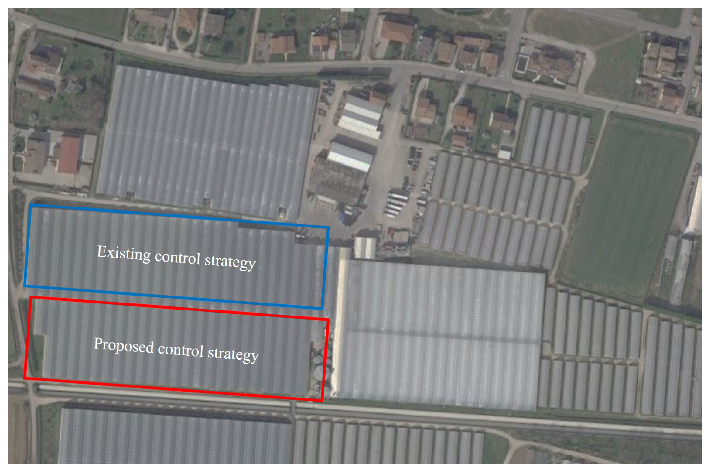
The goal of the paper was twofold. On the one side, the authors aimed at demonstrating how the artificial lighting system of commercial greenhouses represents a great source of electrical power flexibility for DR and DSM strategies. Since switching on or off the artificial lighting system affects the energy demand and the plants’ growth rate, the trade-off between these two variables can be optimized, pursuing the electrical grid needs. This fact represents an additional source of resilience for the electric grid and a clear opportunity to improve the commercial greenhouse profits exploiting energy price fluctuation. On the other hand, the present paper overcomes the scientific literature lack of practical experimental applications of innovative control algorithms for managing commercial greenhouses. The current work is primarily experimental. It describes all the steps required to devise an innovative supervisory algorithm for managing the artificial lighting system of the commercial greenhouse shown in Figure 1, a site in North of Italy (Mantua area, latitude ). The cultivated crop is cherry tomatoes. The controller was implemented in a facility and an experimental campaign was undertaken for almost . The results outlined that the proposed controller is capable to effectively forecast the daylight over the canopy and exploit this prediction to better plan the artificial lights switching on and off. Moreover, simulations over an entire meteorological year highlight how the innovative control strategy may produce of cost saving for the energy traded on the wholesale market.
2. Methodology
Section 2.1 defines which are the primary control goals and constraints that must be considered in the development of the control strategy for the artificial lighting system of a commercial greenhouse. The existing state-of the-art controller based on open-loop indirect feedback strategies is described in Section 2.4. The innovative solution is presented in Section 2.5. It is a supervisory control algorithm capable to evaluate the day-ahead control strategy and to optimize the switching strategy of the artificial lighting system. This fact represents a significant opportunity for saving operative costs and reducing grid unbalances. The controller uses Artificial Intelligence (AI) to identify the primary system dynamics and evaluate how different possible scenarios influence a cost function. The energy tariff—that indicates the energy value and availability—is used directly in a cost function to be optimized. Section 3 details the experimental set-up and the Information and Communication Technologies (ICT) used to implement the controller in the experimental facility. Section 4.1 reports the results carried out during the experimental campaign. To assess the performance of the controller, it was necessary to clearly outline a benchmark strategy. This operation is often tricky for case-studies investigating real implementations of controllers [12]. For this reason, Section 4.2 reports simulated studies to compare the results achievable by means of the proposed solution with the existing state-of the-art controller. Ultimately, Section 5 pinpoints the conclusion of the current work, carefully explaining potential implications and possible future works.
2.1. Plants Interaction with Natural and Artificial Light
Plants’ growth rate is affected by the environmental conditions [16], i.e., air temperature, air relative humidity, carbon dioxide concentration, and light received. In particular, the light in the PAR spectrum is the one involved in the photosynthetic process and influences plant growth. This light can be provided to the plant by the sun or artificial lighting. The goal of the artificial lighting systems is to integrate the natural DLI to enhance crop photosynthetic processes. This relation can be expressed as follows:
where is used to indicate the overall PAR reaching the crop over a period of time. This variable is an energy density [ ] measure referring to the fraction of radiation contained in the PAR spectrum only. is equal to the summation of the DLI and the Artificial Lighting Integral (ALI) contributions at the crop level. Considering a period of time lasting from to , the DLI contribution can be calculated as:
where is the instantaneous natural Photosynthetic Photon Flux Density (PPFD) (Wm passing through the greenhouse cover and reaching the canopy. This value is integrated over the time () obtaining an indication of the energy density (Whm) contained into natural lighting reaching the crop. is a function of the cover lighting transmission properties, the intensity of the external global solar radiation, the direction of the beam solar radiation, the ratio of solar radiation within the PAR spectrum, and the ratio of the diffuse and beam component of the solar radiation. The literature shows how can be derived by the outdoor lighting using the relation proposed by Reference [46]:
This term represents the fraction of daylight filtering through the greenhouse cover and reaching the crop. In the equation, is the Sun elevation angle (always known fixed the commercial greenhouse position and the time-step, expressed in ). is the daylight radiation in the PAR spectrum, and is the ratio of diffuse daylight radiation in the PAR spectrum; both are calculated according to Reference [47]. The variables , , and are coefficients that depends on the properties of the greenhouse (e.g., cover transmission rate or scattering, floor reflection, canopy distance, etc.). They can be estimated using a non-linear multiple regression that retrieves the best-fit values for each case study.
The ALI contribution over the crop can be calculated as:
where is the electrical power adsorbed by the artificial lights in Watts per square meter, is the artificial lighting conversion efficiency expressed in , and is the coefficient of utilization of the artificial lighting that allows to evaluate the share of artificial light effectively reaching the crop over the entire amount of light emitted by the system. Generally, these three variables can be assumed constant and extracted from the integral. is the control variable. It can be either a proportional variable, in case of a dimmerable system, or a Boolean , otherwise.
2.2. The Control Goal
The value of the control variable is defined by the control logic. Pursuing a control goal implies the definition of a set-point trajectory to be tracked. In this case, the control goal is reaching a desired amount of light affecting photosynthesis over a defined interval of time. This goal can be converted into a set-point of the cumulated lighting over the crop, . This value can be substituted in Equation (1):
where is the artificial light required to integrate the natural to reach the predefined set-point. Furthermore, it is necessary to define the horizon of the control (e.g., daily, weekly), setting the integration limits and . Substituting Equations (2) and (4) into Equation (5) and inverting the formulations, it is possible to express the control variable as a function of the other parameters affecting plant physiology:
The solution of this equation is possible once the control goal and the constraints are clearly defined. In addition, in this case, the set-point depends on the control horizon that can be decided arbitrarily by the user (e.g., daily, weekly).
In the experimental activity, this was made possible allowing the end user (i.e., the commercial greenhouse owner or the crop engineers) to interact with the control algorithm through a Graphical User Interface (GUI). The GUI allowed the control goal to be set as the desired daily (expressed in molm or Jm).
2.3. The Controller Constraints
A controller must deal with constraints, like physical limitations of the controlled system or non-viable states defined by the end-users. An always valid constraint was represented by the requirement of having consecutive lighting hours (artificial or natural) to not affect plant physiology. Furthermore, the user was able to set supplemental constraints that can be summarized according to four typologies:
- The maximum number of times that the controller can switch-on and off the artificial lighting system.
- The minimum duration of artificial lighting periods (e.g., I cannot switch on/off the artificial lights every , but they must remain in a constant state for at least ).
- The minimum number of dark hours (i.e., plants need at least some dark hours to assimilate photosynthesis products [48]).
- The hours when artificial lights must be a-priori switched off for reasons external to the primary production process.
2.4. The Existing Control Strategy
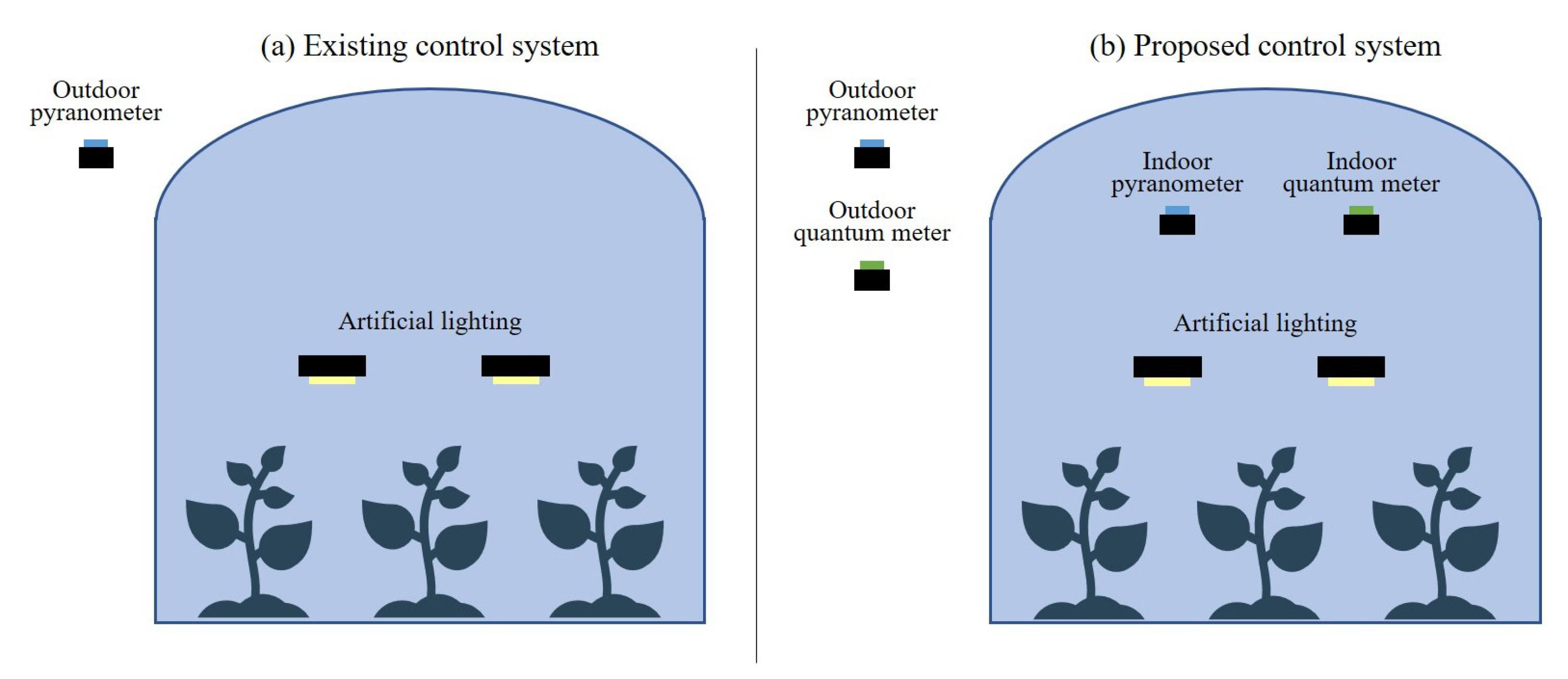
As far as authors knows, the the state-of-the-art control strategy of the artificial lighting control system in commercial greenhouses is a Rule Based Controller (RBC) with an indirect open-loop feedback [49]. Figure 2a describes the control loop used for the existing set-up in the case-study that can be considered representative of the industry state-of-the-art. This solution does not guarantee an optimal performance to reach the control goal described in Section 2.1. Indeed, the control rule does not consider taking advantage by future fluctuations of environmental nor power availability conditions.
For each day of the year, the end user sets the number of hours required, , and the starting time of artificial lighting, . The time of switching-off the artificial lighting system is defined as follows:
is the coefficient of the controller indirect open-loop feedback. It reduces the required daily period of artificial lighting as a function of the natural outside the greenhouse cover. Several thresholds of are arbitrary fixed, and, once reached, the artificial lighting period is reduced by a fixed time-span [50]. For example, the coefficient can be set to satisfy the rule “If the outdoor natural light reaches 12 moles per day, reduce the daily hour of artificial lighting system of 1 h”. These thresholds can be defined by the farmer through the greenhouse computer.
This control logic is affected by two primary drawbacks. First, Equation (6) outlines how the controller goal is based on the integral of a measure. A feed-back controller is intrinsically affected by limitations when it deals with integral measures in the control loop. Contrariwise, this case represents the ideal application for a predictive controller capable to set optimal regulation strategies. Indeed, evaluating the control trajectory over a prediction horizon enables the regulation to exploit potential favorable situations occurring in the future. For example, if the lowest energy tariff would occur at the end of the day, a predictive controller can postpone the artificial lighting period to wait for that moment. The predictive controller is capable of evaluating and forecasting in advance all the disturbances affecting the optimal trajectory to reach the control goal pinpointed by Equation (6) (i.e., and the energy price/availability).
Then, Equation (6) underlines that the feedback of the controller should be based on the DLI over the canopy. However, the variable used in Equation (7) is measured outside the commercial greenhouse cover. This is due to the fact that the shadows of greenhouse construction elements (e.g., vents frames, pillars, and trays) may affect instantaneous measurements, which are used mostly for regulating the fertigation of the crop. The relation between and is defined arbitrarily, with the support of spot measurements, generally repeated during every season (). In this existing control strategy, is measured with a portable PAR-meter and correlated with the measured outside by the Building Automation and Control System (BACS) of the commercial greenhouse. This trivial system may be improved. A method capable of forecasting over the prediction horizon should be developed to implement an effective predictive controller.
2.5. The Proposed Supervisory Predictive Control Strategy
A supervisory predictive control system was proposed and devised to overcome the above-mentioned limitations of the existing state-of–the-art baseline controller. The proposed controller requires monitoring devices that slightly differ from the existing controller needs, as it can be inferred by Figure 2b. Indeed, an additional sensor of light intensity must be integrated inside the greenhouse to improve the controller. The couple of indoor and outdoor sensors may be both pyranometers or quantum sensors, i.e., depending on the light spectrum that should be measured. For the sake of completeness, the present paper used an experimental set-up that had both the possibilities.
The benefits achievable by this novel controller are twofold. On the one side, the controller increases the control strategy awareness of the effects of the cover on natural DLI transmission. In this way, it would be possible to forecast the variable and set-up predictive control strategy. On the other side, this predictive strategy enhances the opportunity to consume energy when it is more available or affordable, enabling DR and DSM strategies.
In discrete time, a predictive controller is formulated according to the following primary elements [11]:
- the measurement time-step that is the time interval between two measures monitored by sensors;
- the control time-step representing the time interval in which the controller is iterated to re-define a new set-point trajectory; and
- the prediction horizon and the control horizon representing the number of future time-steps evaluated in an optimization function; in the present formulation, the two horizons coincide.
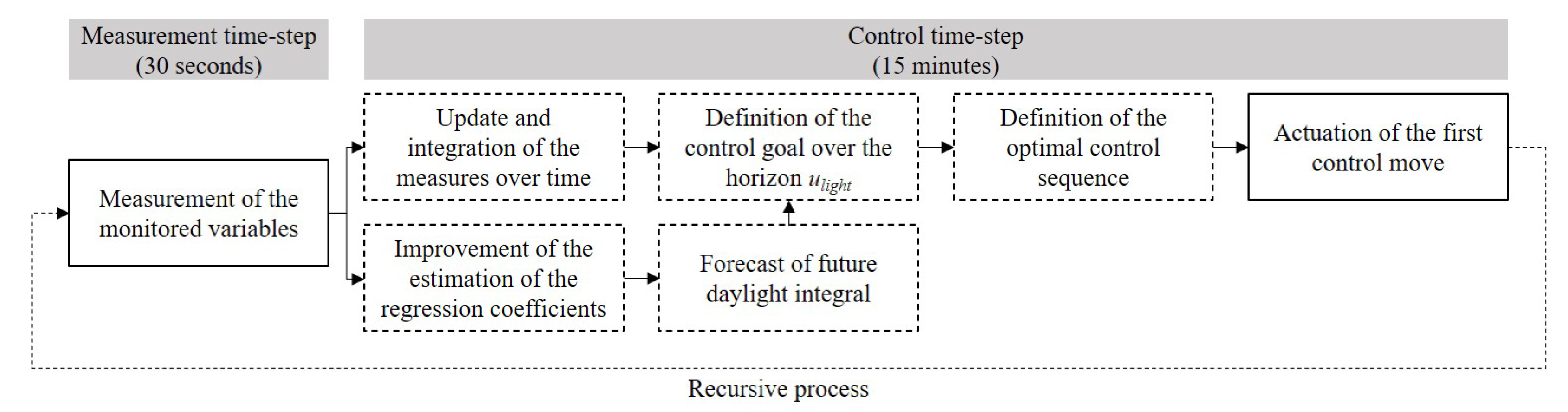
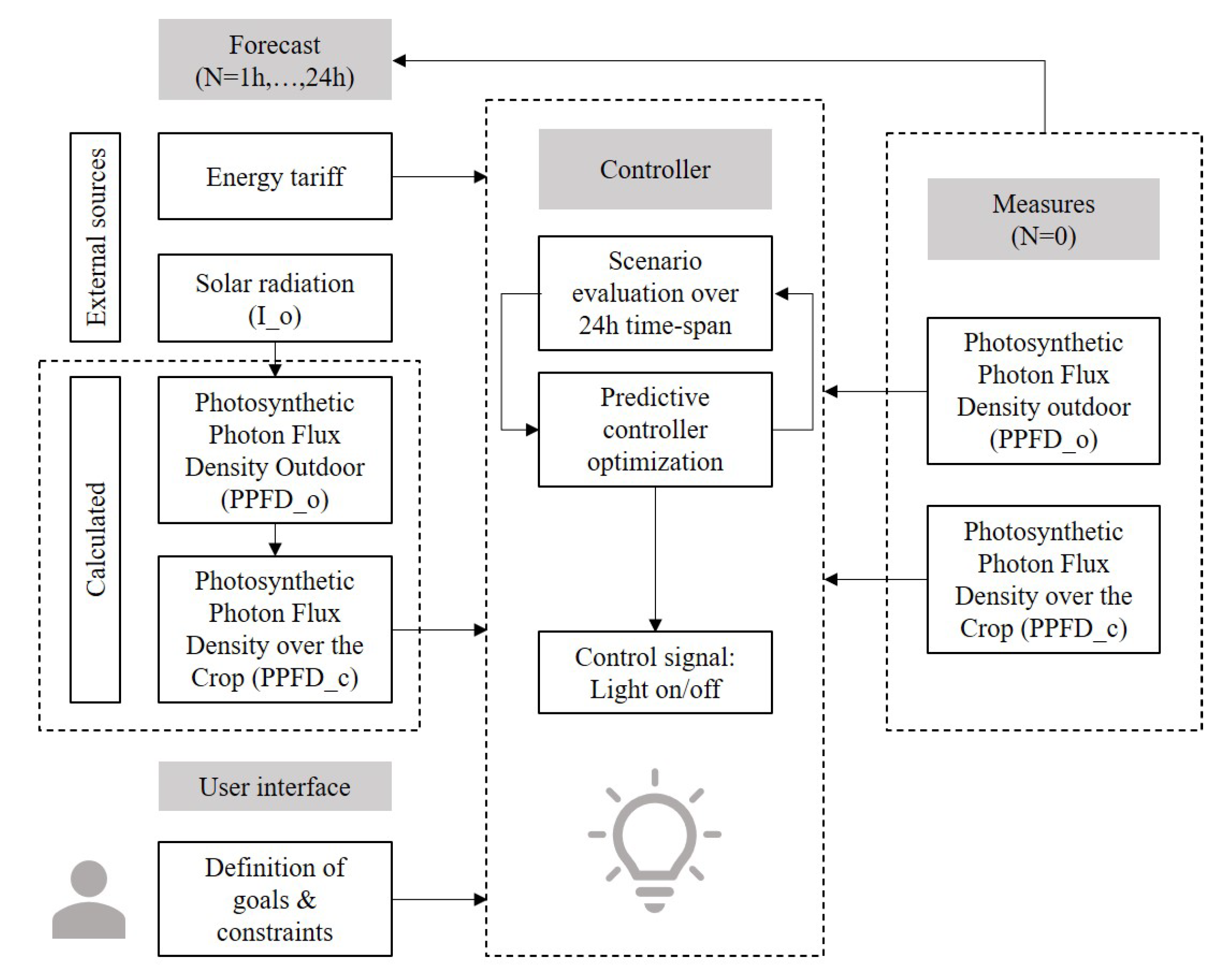
At each control time step, the proposed controller updates the current measures in order to calculate the integral of past values and improve the estimation of the regression coefficients to forecast the daylight radiation filtering into the greenhouse. On the basis of this data, the algorithm re-defines the required control goal, , defined in Equation (6), and subsequently defines the control sequence that optimizes the energy costs. Similarly to the MPC approach, the controller actuates only the first control move and the procedure is repeated according to a receding horizon scheme. The novel algorithm computational steps are pinpointed in Figure 3. Moreover, Figure 4 provides a framework of the variables (measured or regulated) used by the algorithm.
The integral of Equation (6) can be split in two time-spans according to past and future values.
The first of the two integrals in the right side of the previous equation is referred to the past values, of already measured during that day until the current time-step (), and it is named . Once the regulation algorithm retrieves the current measurements from the sensors in the greenhouse, it can calculate the using the previously measured data. becomes a known variable. Every day at midnight, is initialized and set equal to 0.
The second integral, on the right side of Equation (8), is referred to future values, which are the predicted values of from the subsequent control time-step () until the end of the prediction horizon, and it is named . This variable represents the future daylight over the canopy , and it remains the only unknown variable of Equation (6). It is possible to foresee values combining outdoor weather forecast with Equation (3). Indeed, Equation (3) highlights the correlation among the external solar PAR and the daylight over the canopy. The external PAR can be readily predicted using a weather forecast service (i.e., prediction of the radiation in the PAR spectrum can be also easily derived by the forecast overall solar radiation).
The non-linear multiple regression coefficients , , and of Equation (9) are estimated using the minimization of Root Mean Square Error (RMSE) between estimated and monitored data through the Python Numpy library. The estimator evaluates the coefficients that minimize a fitting function represented by least square difference between the measured and the estimated values. data are used as measured inputs, and as calculated inputs, and as measured outputs. Data of the previous are considered in a rolling horizon approach (i.e., the estimation is continuously updated to consider the change over time of the boundary conditions). At least of measurement are necessary to successfully perform the parameters’ identification procedure. The coefficients , , and are constrained . In Reference [16], ; ; were suggested as the reference values for a traditional plastic multi-span greenhouse. Those parameters are used as first attempt values.
Since past values are measured and future values are estimated, all the variables in Equation (6) are known, and the equation becomes:
The term on the left side of Equation (10) does not provide the control sequence directly. However, it is the integral value of , which represents the number of control time-steps when the artificial lighting system has to be switched on from the subsequent time-step () until the end of the control horizon to fulfill the set-point defined by the user. The set-point can be reached following various programs of artificial lights switching on or off. For optimizing this program and reducing the energy cost, the control algorithm has to evaluate all the possible switching on/off scenarios over the prediction horizon and selecting the one that reduces the overall energy costs without violating the controller constraints. The number of possible scenarios is finite. Thus, it is possible to enumerate the maximum number of possible scenarios using combinatorial mathematics:
where, referring to the prediction horizon, n is the total number of control time-steps to the end of the horizon, and k is the number of control time-steps when the artificial lighting system must be switched on. Since , it is possible to retrieve the value of k from Equation (10).
Once the set of possible situations is enumerated, all the unfeasible scenarios are deleted. These situations are those which do not respect the controller constraints. For instance, the user should avoid to switch on the artificial lights for one hour only during the middle of the night, and this case would be considered an unfeasible scenario by the controller. The resulting represents the number of feasible scenarios actually evaluated.
Eventually, the controller defines the scenario that minimizes a cost function represented by the summation of the overall daily energy expenditure. It is possible to formulate the minimize problem as:
where i represents the control time-span interval, and is used to indicate the fluctuating energy tariff in [€/MWh]. If two solutions with the same result exist, the one that anticipated the control goal achievement is selected. Once the optimal control sequence is defined, the next control move is determined unequivocally and applied to the actuators. The remaining part of the control sequence is discarded and recalculated at the next time step in a receding horizon approach.
The control performance was evaluated considering the two more challenging aspects characterizing the algorithm described in Section 2.5. Firstly, the application of Equation (3) required a system identification to be performed by the controller. Secondly, the satisfaction of the conflicting needs intrinsically contained in the control goal presented in Section 2.1. Therefore, on the one hand, the system must minimize the number of hours when the artificial lighting system is consuming energy; on the other hand, a significant decrease of the hours of artificial lighting (ALI) would cause a reduction in the yield production. These two aspects had to be evaluated together.
3. Material and Methods
The methodology presented above was implemented in a real commercial greenhouse. The experimental tests were conducted for 80 days in winter time. The experimental facility was a multi-span plastic greenhouse for the cultivation of tomatoes throughout the year, located in the North Italy (Mantua region, latitude ). The entire facility was , of which were equipped by artificial lights. The greenhouse equipped with an artificial lighting system was divided in two parts of similar size of each, as shown in Figure 1. The one implementing the existing controller was used as a benchmark, and the other one was used to test the proposed controller.
3.1. Hardware Configuration
The lighting system was based on LED Igrox Quantum with a nominal lighting efficiency of and an installed power density of . The overall power supply to the artificial lighting system was distributed over 24 electrical lines at . Artificial lighting were not dimmerable so that the control variable of Equation (8) outlines the schematics of the monitoring and supervisory control units used for this experiment.
The sensing units were represented by two PAR-meters to measure PPFD. The first one was installed outside the commercial greenhouse and labeled as . The second one was installed just over the canopy and labeled as . They were both Apogee SQ-515 Quantum sensors with a sensitivity of /(/), measurement range from 0 to 4000 /, spectral range from 389 to , power supply, and analog signal transmission. The measuring sampling time was set equal to . In parallel, Siap+Micros t055 pyranometers were placed close to the quantum sensors to retrieve data of global solar radiation.
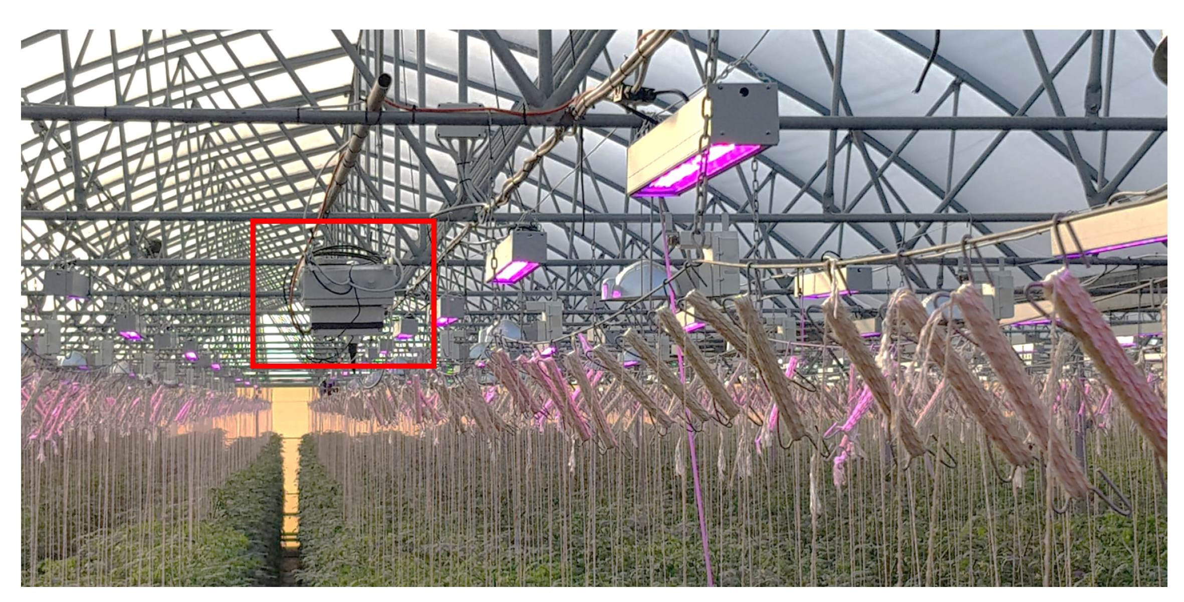
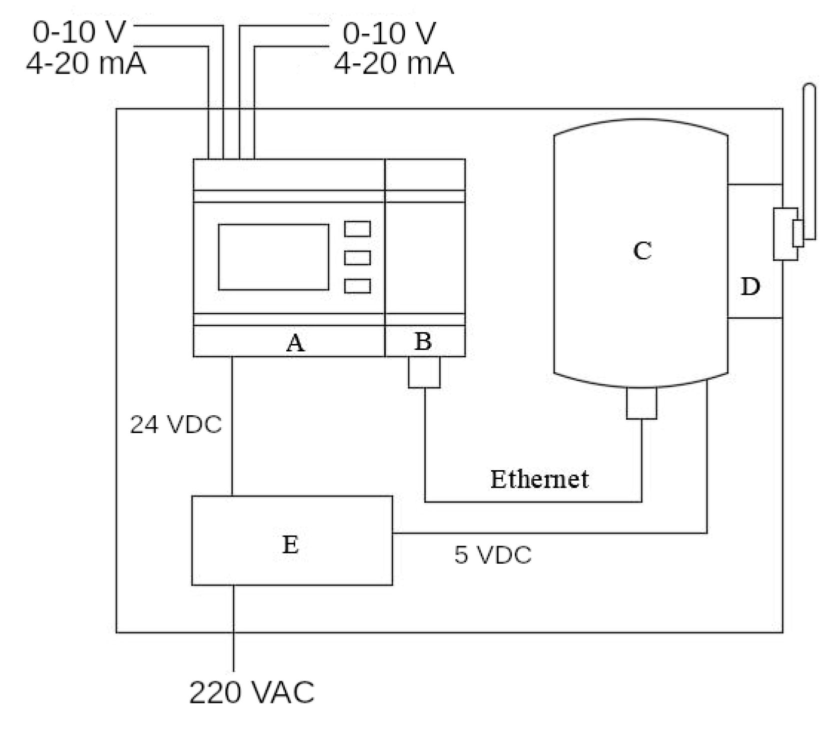
The data acquisition unit was an Industruino IND I/O 1286 enclosed in an electric box installed just over the canopy. The Industruino IND I/O 1286 was selected for its reliability in industrial environments and its GPRS connectivity module. It used two ADC channels to acquire the analog PAR-meter data. Figure 5 shows the monitoring unit installed in the greenhouse during the experimental campaign. Furthermore, Figure 6 is a schematic of the hardware used to integrate the PAR-meters and pyranometers with the greenhouse computer.
3.2. Software Configuration
Once acquired, the signals from the sensors were converted into PPFD measurements and transmitted over GPRS using Message Queue Telemetry Transport (MQTT) protocol. MQTT is one of the most adopted communication protocols for the building Internet of Things (IoT) industry [51]. Those signal were received by an external MQTT broker (For the sake of reliability, the commercial broker provider adafruit.io was used.) and made available through a REST API connection.
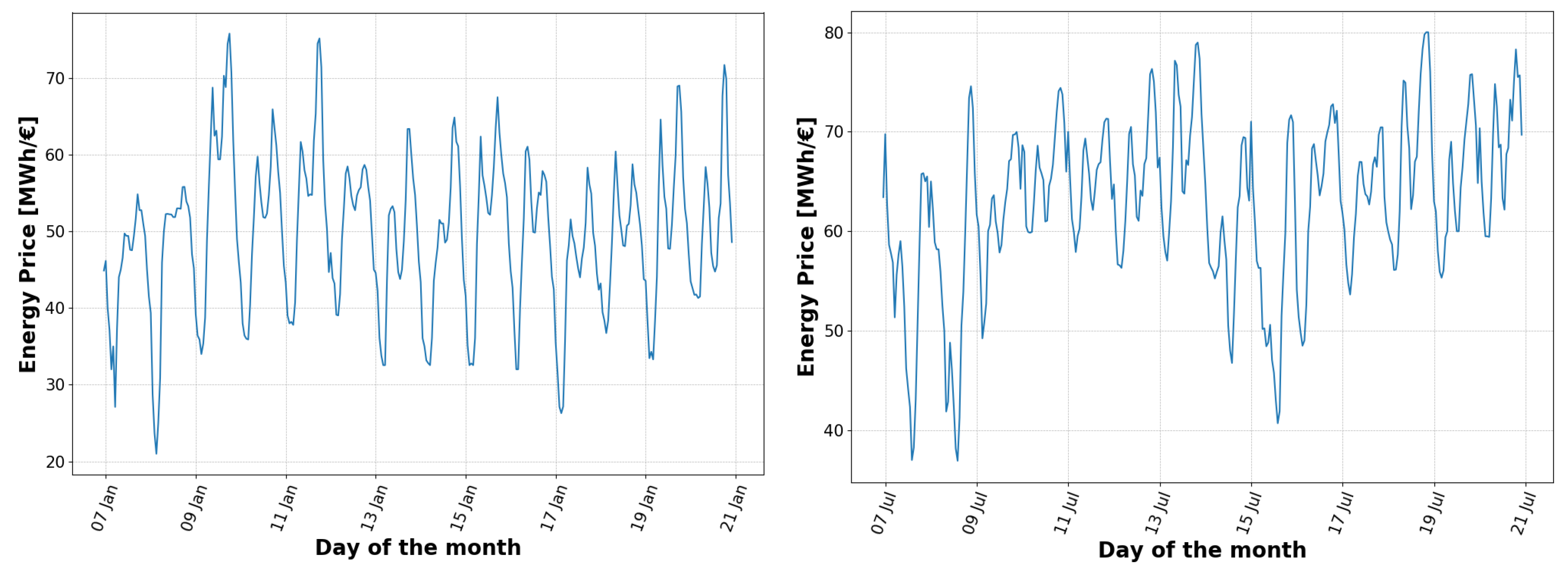
Two external forecasting resources were integrated in the predictive controller. The first one was the day-ahead energy price forecast at the wholesale Italian market [52]. Indeed, the Italian grid regulator (named GME) provides the electric wholesale tariffs of the day-ahead with a sampling time of . Figure 7 shows how the unbalances due to the large penetration of RES caused a great electrical tariff fluctuation over time. The charts show two different weeks. One is characteristic of the winter period, when the experimental tests were undertaken. The other represents a typical summer week, the period of the year when the energy price fluctuation are more significant.
The second forecasting resource integrated was a professional weather prediction service [53]. Foreseen values were available for the next with a sampling time of and updated every by the weather prediction service. The predicted meteorological data were: ambient temperature, ambient relative humidity, atmospheric pressure, wind speed, wind direction, global horizontal solar radiation, diffuse solar radiation, horizontal beam solar radiation, and cloud cover. Only the variables related to solar radiation and cloud cover were actually used by the controller to predict the daylight availability [47]. Correlations among global solar radiation and the solar radiation in the PAR spectrum were used to retrieve indirectly the measurements required.
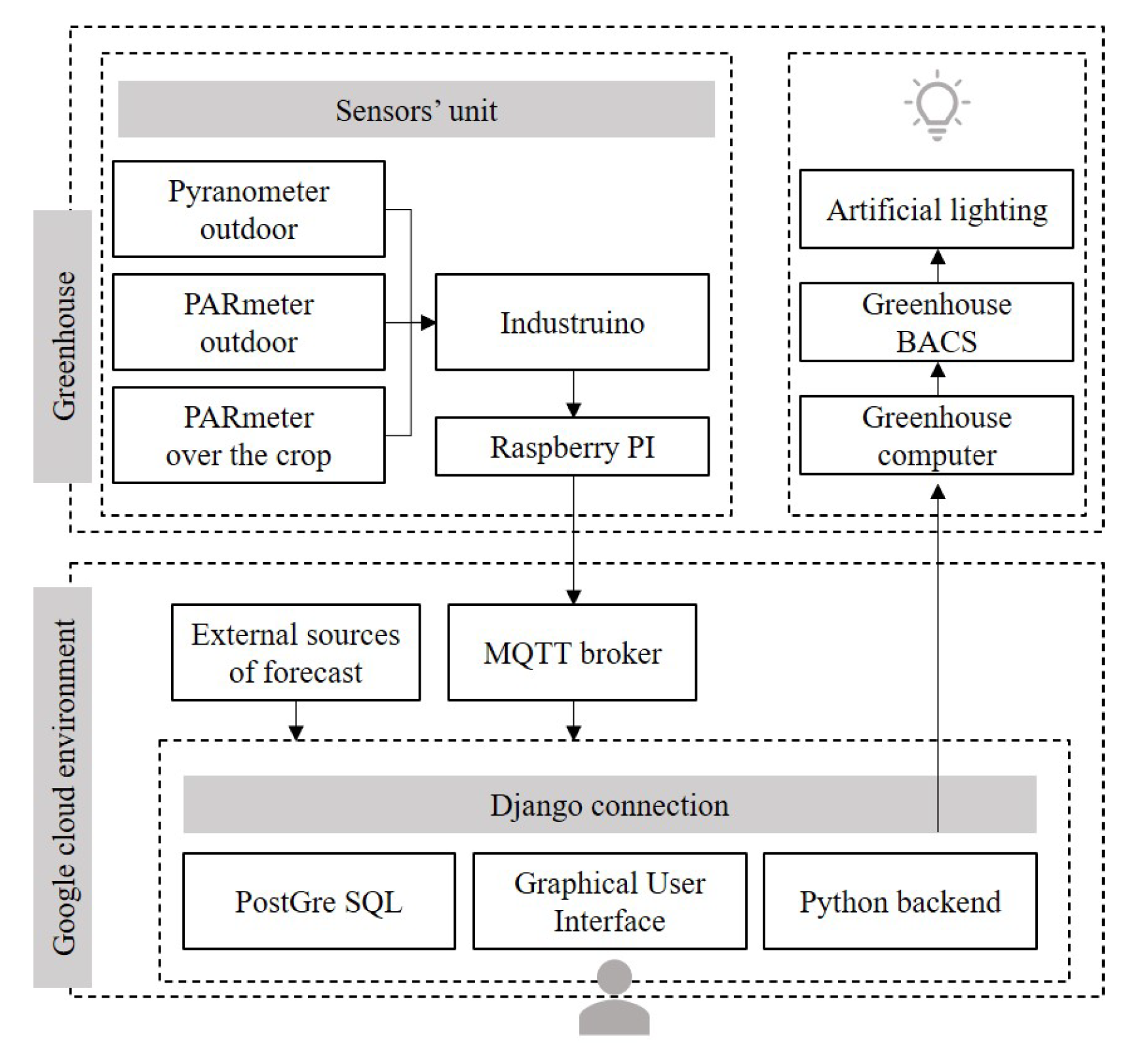
The control logic and database recording were devised firstly using a Raspberry PI—Model B computer installed nearby the cultivation environment and eventually using a virtual machine over Google Cloud server. On the virtual machine, a dedicated service, based on the Phyton Django framework, was used to schedule all the operations. This operation can be summarized into four primary elements:
- Connection with external elements (MQTT broker for sensors, weather-forecast, and price forecast.)
- PostgreSQL database to record the data.
- Python functions to process the data and define the control logic.
- HTML-based GUI to visualize the data and insert user data, goals, and constraints.
The actuation signal for switching On/Off the controlled LED was sent by the Raspberry Pi to the BACS already installed in the greenhouse. This BACS was represented by the commercial solution PRIVA Connext. The connection used a REST API through an software bot installed on the greenhouse computer. This was able to override the input control signal over the Relational DataBase Management System (RDBMS) of the greenhouse computer. The greenhouse computer was directly connected with the BACS that actuated the control signals. The software layer and its respective integration are described in Figure 8.
3.3. Assumptions, Goals, and Constraint Definitions
The only assumption of the present work is considering that the end-user is able to completely benefit from the energy price fluctuation over the wholesale market. Indeed, the wholesale energy price is not the unique component of the energy tariff payed by the end user. The end user tariff includes also additional voices, such as dispatch, taxes, and utilities revenues. However, the wholesale energy price is the component mostly affected by the sharp daily fluctuation of energy availability due to RES penetration. The wholesale market price is a good indicator of the grid unbalances between offer and demand [54]. For this reason, authors limited their benchmark studies to this unique price voice. Measurements were retrieved every 30 s. The control time-step was set equal to 15 min. This means that, every 15-min interval, the algorithm repeats the sequence described in Figure 3. The prediction and control horizon were set equal to 1 day, and at midnight the integral values were reset to 0. The combination of control time-step and prediction horizon length causes the maximum value of n in Equation (11) to be equal to 96, limiting the computational effort of the algorithm. The control goal was set using a daily objective of cumulative . Considering that the experimental campaign was undertaken during the winter season, this value represented a challenging threshold. For the sake of comparison, readers can refer to the outdoor horizontal solar DLI of the location considered. During the experimental campaign period, the daily outdoor DLI ranged between and . When the natural DLI was not sufficient, the artificial lighting system had to integrate the radiation reaching the canopy for boosting crop growth and maintaining the selected set-point.
The primary algorithm constraint was represented by limiting the lighting hours (natural or artificial) to only consecutive periods. This fact strongly reduces the system degrees of freedom. Thus, artificial lights can be switched On during night-time only if the artificial lighting period will be connected with natural DLI dawn or dust. Additional limitations regarding the control effort (i.e., maximum number of times swinging from On to Off and minimum duration of a control move) were not considered. Similarly, there were no periods in which artificial lighting system must be a-priori Off. Eventually, the minimum number of dark hours was set equal to .
4. Results
4.1. Outcomes of the Monitoring Campaign
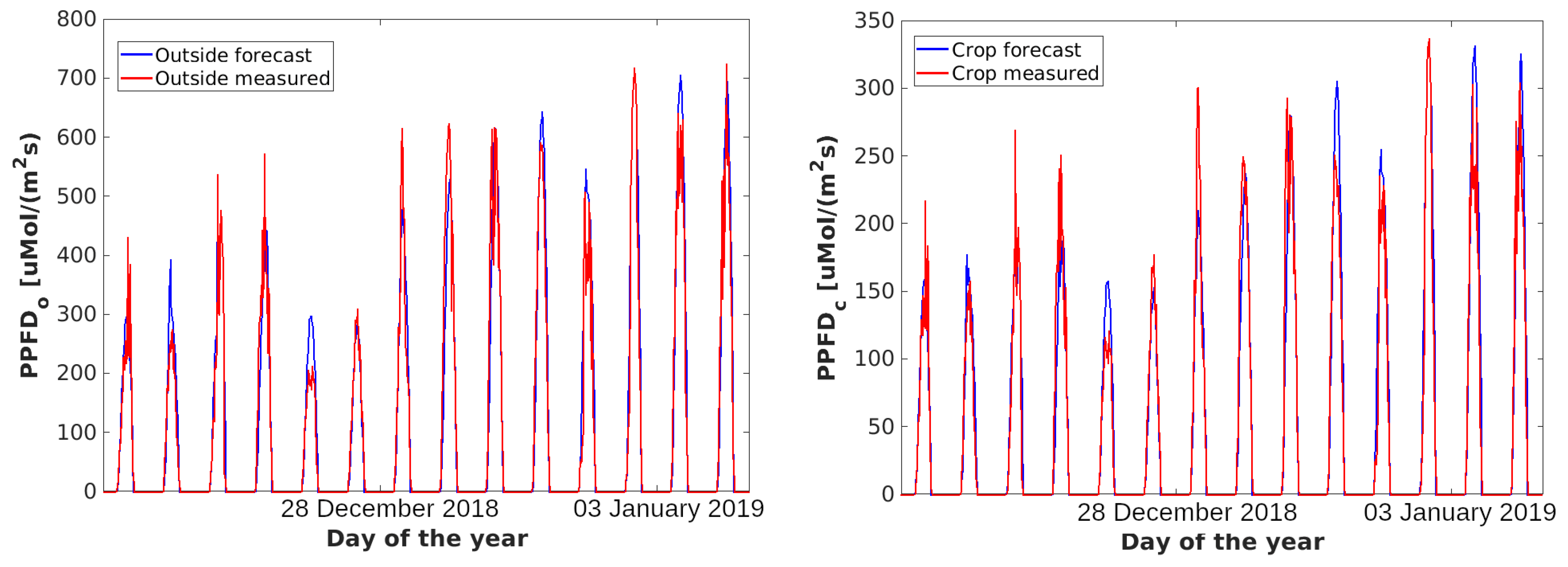
First of all, it is necessary to assess the capability of the forecasting model to estimate the variables (also named external disturbances). Indeed, a predictive controller needs reliable estimations of the future evolution of the system to be robust and enhance its capabilities. Figure 9 allows assessing qualitatively the ability of the algorithm of identifying the parameters affecting the dynamics of the controlled system. For the sake of readability, the chart reports the experimental data over of experimental tests only. The algorithm uses external sources of forecast of solar radiation and current measures to predict the and using Equation (3). The Mean Absolute Percentage Error (MAPE) was used as Key Performance Indicator (KPI) to quantitatively assess the overall system identification capability of the system:
where n is the number of samples considered, is the actual measured value, and is the foreseen value 24-h ahead. The MAPE calculated at the end of the experimental campaign was equal to for and equal to for , underlining the worth estimation capability of the algorithm.
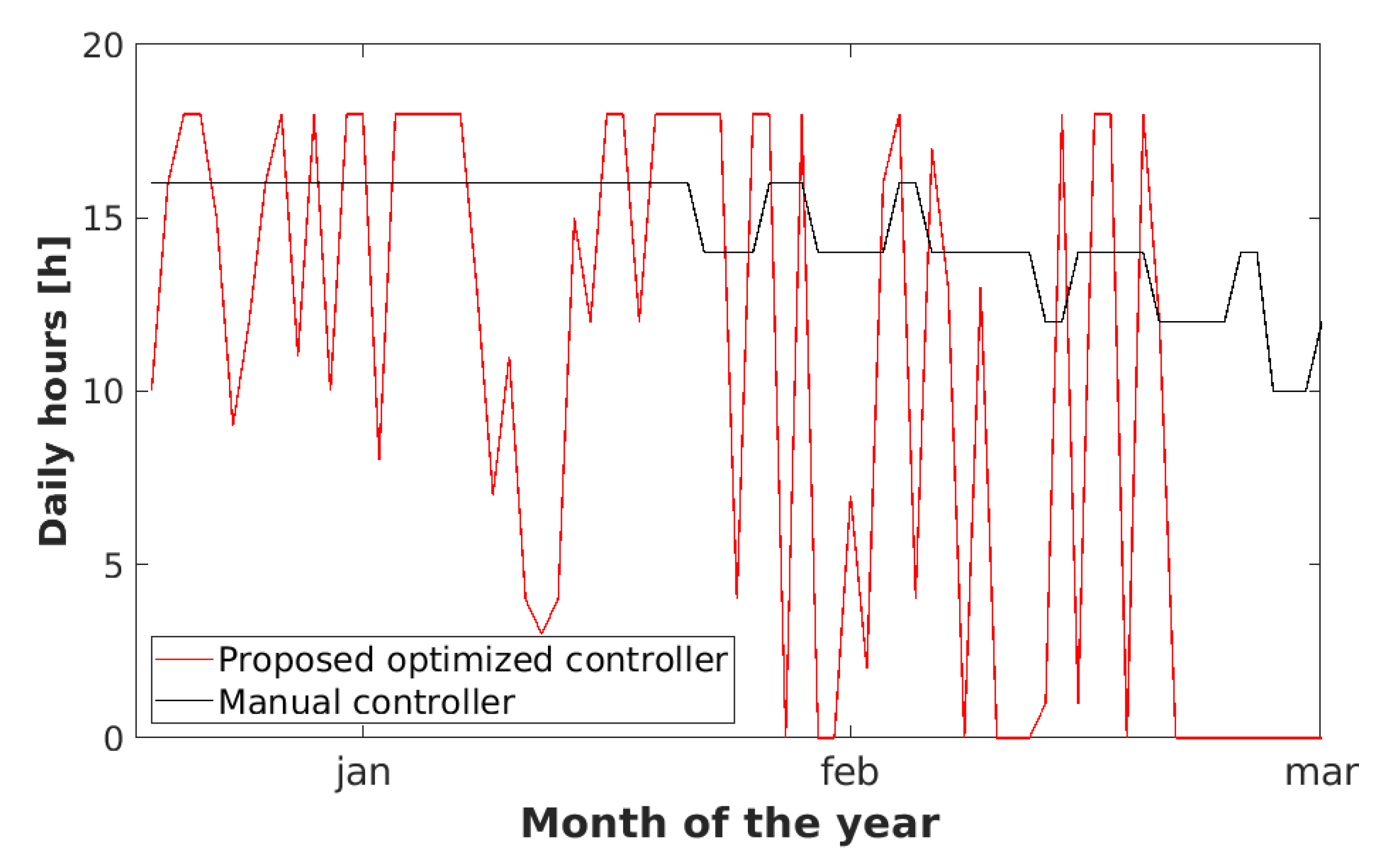
Once the accuracy of the forecast is determined, it is necessary to compare the performance of the proposed predictive controller with the existing one. Figure 10 shows the daily number of hours of artificial lighting system switched On over the entire experimental campaign. This variable was a direct consequence of control action defined by the controller. Red lines represents the results referred to the proposed controller, while the black line represents the behavior of the remaining part of the greenhouse equipped with the traditional controller. The chart highlights two possible situations. The cases when the red line (proposed controller) is below the black line (existing controller) represent those situations when the existing controller provided too much artificial lighting, and the was overtaken. This fact causes additional energy consumption, on the one hand, and a boost of the plant growth, on the other. The opposite situation occurred when the red line is above the red one. Beyond the pros and cons of each situation, the existing control strategy demonstrated its inability to track a user-defined set-point, representing an implicit shortcoming of the regulation strategy. Theoretical simulations were carried out to quantitatively evaluate the difference of performance between the two regulation systems and the DR opportunities offered by commercial greenhouses.
4.2. Year-Long Simulations
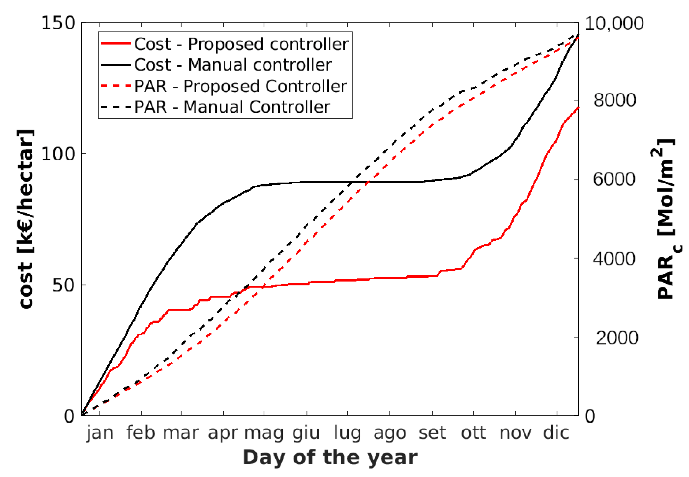
Simulations were deemed necessary for extending the experimental outcomes to results referred to a year-long period. This approach allowed the proposed controller to be compared in detail with the existing state-of-the-art regulation strategy. The energy wholesale prices for 2018 were used for this purpose. A Typical Meteorological Year (TMY) from the International Weather for Energy Calculation (IWEC) was used as a reference to perform these simulations. Among the available locations, the Brescia-Ghedi was the closest to the experimental facility. A simple simulation environment was set up in Phyton to simulate the behavior of the existing state-of-the-art controller. This operation was simple since the existing controller was based on an open-loop feedback RBC requiring external variables only to compute the control moves. Figure 11 highlights the outcomes obtained by those simulations.
The two conflicting goals of the control algorithm are reported on the chart. On the one side, the continuous lines indicate the accumulated cost for supply energy to the artificial lighting system. On the other side, dashed lines are used to indicated the accumulated PAR reaching the crop due to the integration of natural and artificial lighting. The trends outline how the proposed approach allows the overall cost of artificial lighting to be reduced keeping throughout the year a comparable level of PAR reaching the crop. The proposed optimized controller reduced by the energy cost, while it guaranteed that the cumulative DLI reaching the crop is affected for only. The proposed solution was particularly effective in months from March to April and from September to November. This is due to the easy prediction of lighting in those periods. The system proposed, thanks to the short-term control of indoor light, was able to reduce visibly the employment of artificial lights when not needed, consequently reducing the costs.
5. Conclusions
The current work is focused on commercial greenhouses equipped with artificial lighting systems. Regulating these artificial lights with predictive optimized control algorithms could enhance important energy and cost saving. Furthermore, this typology of greenhouses was individuated as a significant source of energy flexibility to participate to DR and DSM programs. The recent advent of efficient and economic LED technology has fostered a widespread adoption of artificial light to integrate the natural PAR reaching the crop. A power density over is necessary to provide enough light to ensure plant growth even with the more advanced artificial lighting system installed. Thus, energy and power demand of such typology of greenhouses became really significant.
The present paper used a multi-span plastic greenhouse located in North Italy as an experimental case-study. In particular, the study was focused on two zones of the greenhouse measuring each. Both these zones were equipped with the same LED artificial lighting system requiring an overall electrical power supply around . In one of the two zones, the state-of-the-art existing controller was maintained to be used as a benchmark. A novel predictive and optimized control system for artificial lighting was formulated and devised into the remaining zone. This controller uses a recursive regression algorithm to estimate the amount of natural lighting reaching the crop. Afterwards, combinatorial calculation was used to individuate the scenario of artificial lighting regulation that allowed a threshold of minimum daily PAR to be reached at the minimum the energy cost. Year-long simulation showed that the proposed algorithm over-performed the existing regulation strategy, enabling energy cost saving up to .
The control algorithm was also implemented into the case-study using a low-cost monitoring hardware, which was coupled with the control system of the greenhouse computer. This aspect represents a practical demonstration of how current technologies can be readily integrated using embedded controller and open communication protocols. At the same time, the presented study provides an experimental demonstration of the validity of the controller through the comparison of the performance of the predictive controller against the baseline regulation strategy. The use of a simplified simulation model allowed the result to be year-long extended and highlighted how the proposed controller might outperform the state-of-the-art existing regulation logic of the greenhouse artificial lights. The proposed predictive controller enhancing the energy flexibility of the greenhouse transforming it in a facility that may provide DSM and DR services to the electrical grid. This services are significant due to the high power required by artificial lights and the possibility of a very fast response that does not affect considerably the primary controlled process (i.e., plants’ growth). For this reason, the present paper aimed to individuate greenhouses equipped with artificial lights as a very important element for the balancing of future electrical grids.
Future works will focus on two goals. On the one side, the data monitoring hardware will be optimized and simplified to further reduce the costs and allow a more capillary monitoring within the wide greenhouse environment. Furthermore, this electronic development will also consider the adoption of Low Power Wide Area Network (LPWAN) (e.g., SigFox, LoRa) to further reduce the power consumption of the deployed sensors. On the other side, the algorithm will be extended to consider other variables affecting plants’ growth, such as the indoor air temperature, relative humidity, and carbon dioxide concentration.
Author Contributions
Conceptualization, G.S. and E.G.; Formal analysis, L.G.; Funding acquisition, E.G.; Methodology, G.S., L.G., and E.F.; Software, G.S. and L.G.; Supervision, E.G. and E.F.; Writing—original draft, G.S.; Writing—review & editing, G.S., L.G., and E.F. All authors have read and agreed to the published version of the manuscript.
Funding
This research received no external funding.
Institutional Review Board Statement
Not applicable.
Informed Consent Statement
Not applicable.
Data Availability Statement
The data presented in this study are available on request from the corresponding author.
Acknowledgments
Authors strongly acknowledge Vitangelo Di Pierro and Mattia Tononi of Ageon Tech for the agronomic support and Alessandro Olivieri of Igrox for providing the monitoring equipment.
Conflicts of Interest
The authors declare no conflict of interest.
Abbreviations
The following abbreviations are used in the text:
| RES | Renewable Energy Sources |
| DSM | Demand Side Management |
| DR | Demand Response |
| PV | PhotoVoltaic |
| AI | Artificial Intelligence |
| PPFD | Photosynthetic Photon Flux Density |
| TMY | Typical Meteorological Year |
| PAR | Photosynthetic Active Radiation |
| ADC | Analog signal to Digital signal Converter |
| MQTT | Message Queue Telemetry Transport |
| BACS | Building Automation and Control System |
| DLI | DayLight Integral |
| RBC | Rule Based Controller |
| RDBMS | Relational DataBase Management System |
| GUI | Graphical User Interface |
| HVAC | Heating Ventilating and Air Conditioning |
| MPC | Model Predictive Control |
| LED | Light Emitting Diode |
| ALI | Artificial Lighting Integral |
| IoT | Internet of Things |
| ICT | Information and Communication Technologies |
| EPW | Energy Plus Weather file |
| KPI | Key Performance Indicator |
| MAPE | Mean Absolute Percentage Error |
| LPWAN | Low Power Wide Area Network |
| RMSE | Root Mean Square Error |
| IWEC | International Weather for Energy Calculations |
References
- Golzar, F.; Heeren, N.; Hellweg, S.; Roshandel, R. A comparative study on the environmental impact of greenhouses: A probabilistic approach. Sci. Total Environ. 2019, 675, 560–569. [Google Scholar] [CrossRef]
- Dias, G.M.; Ayer, N.W.; Khosla, S.; Van Acker, R.; Young, S.B.; Whitney, S.; Hendricks, P. Life cycle perspectives on the sustainability of Ontario greenhouse tomato production: Benchmarking and improvement opportunities. J. Clean. Prod. 2017, 140, 831–839. [Google Scholar] [CrossRef]
- Golzar, F.; Heeren, N.; Hellweg, S.; Roshandel, R. A novel integrated framework to evaluate greenhouse energy demand and crop yield production. Renew. Sustain. Energy Rev. 2018, 96, 487–501. [Google Scholar] [CrossRef]
- Fabrizio, E. Energy reduction measures in agricultural greenhouses heating: Envelope, systems and solar energy collection. Energy Build. 2012, 53, 57–63. [Google Scholar] [CrossRef]
- Critten, D.; Bailey, B. A review of greenhouse engineering developments during the 1990s. Agric. For. Meteorol. 2002, 112, 1–22. [Google Scholar] [CrossRef]
- Zhang, Y.; Gauthier, L.; De Halleux, D.; Dansereau, B.; Gosselin, A. Effect of covering materials on energy consumption and greenhouse microclimate. Agric. For. Meteorol. 1996, 82, 227–244. [Google Scholar] [CrossRef]
- Rasheed, A.; Na, W.H.; Lee, J.W.; Kim, H.T.; Lee, H.W. Optimization of Greenhouse Thermal Screens For Maximized Energy Conservation. Energies 2019, 12, 3592. [Google Scholar] [CrossRef] [Green Version]
- Rabbi, B.; Chen, Z.H.; Sethuvenkatraman, S. Protected Cropping in Warm Climates: A Review of Humidity Control and Cooling Methods. Energies 2019, 12, 2737. [Google Scholar] [CrossRef] [Green Version]
- Benli, H.; Durmuş, A. Evaluation of ground-source heat pump combined latent heat storage system performance in greenhouse heating. Energy Build. 2009, 41, 220–228. [Google Scholar] [CrossRef]
- Yano, A.; Cossu, M. Energy sustainable greenhouse crop cultivation using photovoltaic technologies. Renew. Sustain. Energy Rev. 2019, 109, 116–137. [Google Scholar] [CrossRef]
- Serale, G.; Fiorentini, M.; Capozzoli, A.; Bernardini, D.; Bemporad, A. Model predictive control (MPC) For enhancing building and HVAC system energy efficiency: Problem formulation, applications and opportunities. Energies 2018, 11, 631. [Google Scholar] [CrossRef] [Green Version]
- Serale, G.; Fiorentini, M.; Capozzoli, A.; Cooper, P.; Perino, M. Formulation of a model predictive control algorithm to enhance the performance of a latent heat solar thermal system. Energy Convers. Manag. 2018, 173, 438–449. [Google Scholar] [CrossRef]
- Fiorentini, M.; Serale, G.; Kokogiannakis, G.; Capozzoli, A.; Cooper, P. Development and evaluation of a comfort-oriented control strategy for thermal management of mixed-mode ventilated buildings. Energy Build. 2019, 202, 109347. [Google Scholar] [CrossRef]
- Serale, G.; Fiorentini, M.; Noussan, M. Development of algorithms For building energy efficiency. In Start-Up Creation, 2nd ed.; Pacheco-Torgal, F., Rasmussen, E., Granqvist, C.G., Ivanov, V., Kaklauskas, A., Makonin, S., Eds.; Woodhead Publishing Series in Civil and Structural Engineering; Woodhead Publishing: Cambridge, UK, 2020; pp. 267–290. [Google Scholar] [CrossRef]
- Kochhar, A.; Kumar, N. Wireless sensor networks For greenhouses: An end-to-end review. Comput. Electron. Agric. 2019, 163, 104877. [Google Scholar] [CrossRef]
- Van Straten, G.; van Willigenburg, G.; van Henten, E.; van Ooteghem, R. Optimal Control of Greenhouse Cultivation; CRC Press: Boca Raton, FL, USA, 2010. [Google Scholar]
- Van Henten, E. Greenhouse Climate Management: An Optimal Control Approach. Ph.D. Thesis, Wageningen University, Wageningen, The Netherlands, 1994. [Google Scholar]
- Van Henten, E. Sensitivity analysis of an optimal control problem in greenhouse climate management. Biosyst. Eng. 2003, 85, 355–364. [Google Scholar] [CrossRef]
- Shen, Y.; Wei, R.; Xu, L. Energy consumption prediction of a greenhouse and optimization of daily average temperature. Energies 2018, 11, 65. [Google Scholar] [CrossRef] [Green Version]
- Maher, A.; Kamel, E.; Enrico, F.; Atif, I.; Abdelkader, M. An intelligent system For the climate control and energy savings in agricultural greenhouses. Energy Effic. 2016, 9, 1241–1255. [Google Scholar] [CrossRef]
- Revathi, S.; Sivakumaran, N. Fuzzy based temperature control of greenhouse. IFAC Pap. 2016, 49, 549–554. [Google Scholar] [CrossRef]
- Tang, Y.; Jia, M.; Mei, Y.; Yu, Y.; Zhang, J.; Tang, R.; Song, K. 3D intelligent supplement light illumination using hybrid sunlight and LED For greenhouse plants. Optik 2019, 183, 367–374. [Google Scholar] [CrossRef]
- Ma, D.; Carpenter, N.; Maki, H.; Rehman, T.U.; Tuinstra, M.R.; Jin, J. Greenhouse environment modeling and simulation For microclimate control. Comput. Electron. Agric. 2019, 162, 134–142. [Google Scholar] [CrossRef]
- Chen, L.; Du, S.; He, Y.; Liang, M.; Xu, D. Robust model predictive control For greenhouse temperature based on particle swarm optimization. Inf. Process. Agric. 2018, 5, 329–338. [Google Scholar] [CrossRef]
- Blasco, X.; Martínez, M.; Herrero, J.M.; Ramos, C.; Sanchis, J. Model-based predictive control of greenhouse climate For reducing energy and water consumption. Comput. Electron. Agric. 2007, 55, 49–70. [Google Scholar] [CrossRef]
- Xu, D.; Du, S.; van Willigenburg, L.G. Optimal control of Chinese solar greenhouse cultivation. Biosyst. Eng. 2018, 171, 205–219. [Google Scholar] [CrossRef]
- Xu, D.; Du, S.; van Willigenburg, G. Adaptive two time-scale receding horizon optimal control for greenhouse lettuce cultivation. Comput. Electron. Agric. 2018, 146, 93–103. [Google Scholar] [CrossRef]
- Xu, D.; Du, S.; van Willigenburg, G. Double closed-loop optimal control of greenhouse cultivation. Control Eng. Pract. 2019, 85, 90–99. [Google Scholar] [CrossRef]
- Bersani, C.; Ouammi, A.; Sacile, R.; Zero, E. Model Predictive Control of Smart Greenhouses as the Path towards Near Zero Energy Consumption. Energies 2020, 13, 3647. [Google Scholar] [CrossRef]
- Körner, O.; Heuvelink, E.; Niu, Q. Quantification of temperature, CO2, and light effects on crop photosynthesis as a basis For model-based greenhouse climate control. J. Hortic. Sci. Biotechnol. 2009, 84, 233–239. [Google Scholar] [CrossRef]
- Heuvelink, E.; Challa, H. Dynamic optimization of artificial lighting in greenhouses. Int. Symp. Growth Yield Control Veg. Prod. 1989, 260, 401–412. [Google Scholar] [CrossRef] [Green Version]
- van Iersel, M.W. Optimizing LED lighting in controlled environment agriculture. In Light Emitting Diodes for Agriculture; Springer: Singapore, 2017; pp. 59–80. [Google Scholar]
- Paucek, I.; Pennisi, G.; Pistillo, A.; Appolloni, E.; Crepaldi, A.; Calegari, B.; Spinelli, F.; Cellini, A.; Gabarrell, X.; Orsini, F.; et al. Supplementary LED interlighting improves yield and precocity of greenhouse tomatoes in the Mediterranean. Agronomy 2020, 10, 1002. [Google Scholar] [CrossRef]
- Singh, D.; Basu, C.; Meinhardt-Wollweber, M.; Roth, B. LEDs For energy efficient greenhouse lighting. Renew. Sustain. Energy Rev. 2015, 49, 139–147. [Google Scholar] [CrossRef] [Green Version]
- Berkovich, Y.A.; Konovalova, I.; Smolyanina, S.; Erokhin, A.; Avercheva, O.; Bassarskaya, E.; Kochetova, G.; Zhigalova, T.; Yakovleva, O.; Tarakanov, I. LED crop illumination inside space greenhouses. Reach 2017, 6, 11–24. [Google Scholar] [CrossRef]
- Nelson, J.A.; Bugbee, B. Economic Analysis of Greenhouse Lighting: Light Emitting Diodes vs. High Intensity Discharge Fixtures. PLoS ONE 2014, 9. [Google Scholar] [CrossRef] [PubMed] [Green Version]
- Jordehi, A.R. Optimisation of demand response in electric power systems, a review. Renew. Sustain. Energy Rev. 2019, 103, 308–319. [Google Scholar] [CrossRef]
- Dranka, G.G.; Ferreira, P. Review and assessment of the different categories of demand response potentials. Energy 2019, 179, 280–294. [Google Scholar] [CrossRef]
- Yan, X.; Ozturk, Y.; Hu, Z.; Song, Y. A review on price-driven residential demand response. Renew. Sustain. Energy Rev. 2018, 96, 411–419. [Google Scholar] [CrossRef]
- Lu, X.; Zhou, K.; Zhang, X.; Yang, S. A systematic review of supply and demand side optimal load scheduling in a smart grid environment. J. Clean. Prod. 2018, 203, 757–768. [Google Scholar] [CrossRef]
- Cui, H.; Zhou, K. Industrial power load scheduling considering demand response. J. Clean. Prod. 2018, 204, 447–460. [Google Scholar] [CrossRef]
- Chen, Y.; Xu, P.; Gu, J.; Schmidt, F.; Li, W. Measures to improve energy demand flexibility in buildings For demand response (DR): A review. Energy Build. 2018, 177, 125–139. [Google Scholar] [CrossRef]
- Tsay, C.; Kumar, A.; Flores-Cerrillo, J.; Baldea, M. Optimal demand response scheduling of an industrial air separation unit using data-driven dynamic models. Comput. Chem. Eng. 2019, 126, 22–34. [Google Scholar] [CrossRef] [Green Version]
- Jung, W.; Jazizadeh, F. Human-in-the-loop HVAC operations: A quantitative review on occupancy, comfort, and energy-efficiency dimensions. Appl. Energy 2019, 239, 1471–1508. [Google Scholar] [CrossRef]
- Lv, C.; Yu, H.; Li, P.; Wang, C.; Xu, X.; Li, S.; Wu, J. Model predictive control based robust scheduling of community integrated energy system with operational flexibility. Appl. Energy 2019, 243, 250–265. [Google Scholar] [CrossRef]
- De Zwart, H. Analyzing Energy-Saving Options in Greenhouse Cultivation Using a Simulation Model. Ph.D. Dissertation, University of Wageningen, Wageningen, The Netherlands, 1996. [Google Scholar]
- Gijzen, H.; Heuvelink, E.; Challa, H.; Marcelis, L.; Dayan, E.; Cohen, S.; Fuchs, M. Hortisim: A model For greenhouse crops and greenhouse climate. Model. Plant Growth Environ. Control Farm Manag. Prot. Cultiv. 1997, 456, 441–450. [Google Scholar] [CrossRef] [Green Version]
- Körner, O.; Challa, H.; van Ooteghem, R.J. Modelling temperature effects on crop photosynthesis at high radiation in a solar greenhouse. Acta Hortic. 2003, 137–144. [Google Scholar] [CrossRef]
- van Ittersum, M.K.; Leffelaar, P.A.; van Keulen, H.; Kropff, M.J.; Bastiaans, L.; Goudriaan, J. On approaches and applications of the Wageningen crop models. Eur. J. Agron. 2003, 18, 201–234. [Google Scholar] [CrossRef]
- Faust, J.E. First Research Report. Light management in greenhouses. Available online: www.specmeters.com/assets/1/7/A051.pdf (accessed on 1 December 2020).
- Froiz-Míguez, I.; Fernández-Caramés, T.; Fraga-Lamas, P.; Castedo, L. Design, implementation and practical evaluation of an IoT home automation system For fog computing applications based on MQTT and ZigBee-WiFi sensor nodes. Sensors 2018, 18, 2660. [Google Scholar] [CrossRef] [PubMed] [Green Version]
- Day Ahead Market Forecast. 2019. Available online: www.mercatoelettrico.org (accessed on 1 December 2020).
- Weather Forecast Single Access Point. 2019. Available online: www.lrcservizi.it (accessed on 30 July 2018).
- Poruschi, L.; Ambrey, C.L.; Smart, J.C. Revisiting feed-in tariffs in Australia: A review. Renew. Sustain. Energy Rev. 2018, 82, 260–270. [Google Scholar] [CrossRef]
Figure 1.
Overview of the greenhouse where the experimental setup was installed.

Figure 2.
(a) The existing control open-loop including an outdoor sensor only. (b) The proposed control system.
Figure 2.
(a) The existing control open-loop including an outdoor sensor only. (b) The proposed control system.

Figure 3.
Computational steps of the proposed controller.

Figure 4.
Framework of the variables used by the proposed control algorithm. The arrow connecting the measures box with the forecast one indicates that current monitored variables are used to tailor the prediction of their future values.
Figure 4.
Framework of the variables used by the proposed control algorithm. The arrow connecting the measures box with the forecast one indicates that current monitored variables are used to tailor the prediction of their future values.

Figure 5.
Sensors installed inside the greenhouse with the electrical cabinet containing the data monitoring unit hanged to the greenhouse cover.
Figure 5.
Sensors installed inside the greenhouse with the electrical cabinet containing the data monitoring unit hanged to the greenhouse cover.

Figure 6.
Schematic of the monitoring unit. (A) Industruino IND I/O 1286; (B) Industruino Ethernet module; (C) Raspberry PI Model 3; (D) GPRS unit; (E) power supply. The two 4–20 mA connections acquire the data from the indoor and outdoor pyranometers; the two 0–10 V connections acquire the data from the indoor and outdoor Photosynthetic Active Radiation (PAR)-meters.

Figure 7.
(left) Wholesale energy market price trends for the weeks from 7 to 21 January 2019. (right) Wholesale energy market price trends for the weeks from 7 to 21 July 2018.
Figure 7.
(left) Wholesale energy market price trends for the weeks from 7 to 21 January 2019. (right) Wholesale energy market price trends for the weeks from 7 to 21 July 2018.

Figure 8.
Schematic of the software layers and their respective integration in the controller.

Figure 9.
System identification. Red lines indicate the natural horizontal solar radiation. Dashed lines are the values estimated 24-h ahead by the proposed algorithm. The figure on the left indicates the outdoor solar radiation () measured and computed. The figure on the right indicates the solar radiation over the canopy ().

Figure 10.
The daily number of hours of artificial lighting system switched on. The black line indicates the existing state-of-the-art controller, while the red line is the control sequence defined and implemented by the proposed controller.
Figure 10.
The daily number of hours of artificial lighting system switched on. The black line indicates the existing state-of-the-art controller, while the red line is the control sequence defined and implemented by the proposed controller.

Figure 11.
Year-long simulation and evaluation of the satisfaction of control goals. Black lines refer to the existing state-of-the-art controller, while red lines refer to the proposed controller. Dashed lines indicate the cumulative reaching the crop; Continuous lines indicate cumulative electrical energy cost.

Publisher’s Note: MDPI stays neutral with regard to jurisdictional claims in published maps and institutional affiliations. |
© 2021 by the authors. Licensee MDPI, Basel, Switzerland. This article is an open access article distributed under the terms and conditions of the Creative Commons Attribution (CC BY) license (http://creativecommons.org/licenses/by/4.0/).
Share and Cite
MDPI and ACS Style
Serale, G.; Gnoli, L.; Giraudo, E.; Fabrizio, E. A Supervisory Control Strategy for Improving Energy Efficiency of Artificial Lighting Systems in Greenhouses. Energies 2021, 14, 202. https://0-doi-org.brum.beds.ac.uk/10.3390/en14010202
AMA Style
Serale G, Gnoli L, Giraudo E, Fabrizio E. A Supervisory Control Strategy for Improving Energy Efficiency of Artificial Lighting Systems in Greenhouses. Energies. 2021; 14(1):202. https://0-doi-org.brum.beds.ac.uk/10.3390/en14010202
Chicago/Turabian StyleSerale, Gianluca, Luca Gnoli, Emanuele Giraudo, and Enrico Fabrizio. 2021. "A Supervisory Control Strategy for Improving Energy Efficiency of Artificial Lighting Systems in Greenhouses" Energies 14, no. 1: 202. https://0-doi-org.brum.beds.ac.uk/10.3390/en14010202
Note that from the first issue of 2016, this journal uses article numbers instead of page numbers. See further details here.