Dual and Ternary Biofuel Blends for Desalination Process: Emissions and Heat Recovered Assessment

Mechanical Engineering Department, College of Engineering, Taif University, P.O. Box 11099, Taif 21944, Saudi Arabia
Energies 2021, 14(1), 61; https://0-doi-org.brum.beds.ac.uk/10.3390/en14010061
Submission received: 25 November 2020
/
Revised: 19 December 2020
/
Accepted: 22 December 2020
/
Published: 24 December 2020
(This article belongs to the Special Issue Waste-to-Wheel Approach for Future Renewable Drop-In Fuel Development)
Abstract
:Desalination using fossil fuels is so far the most common technique for freshwater production worldwide. However, such a technique faces some challenges due to limited fossil fuels, high pollutants in our globe, and its high energy demand. In this study, solutions for such challenges were proposed and investigated. Renewable biofuel blends were introduced and examined as energy/sources for desalination plants and, in turn, reduced dependency on fossil fuels, enhanced pollutants, and recovered energy for desalinations. Eight different blended biofuels in terms of dual and ternary blend approaches were investigated. Results displayed that dual and ternary blends of gasoline/n-butanol, gasoline/isobutanol, gasoline/n-butanol/isobutanol, gasoline/bioethanol/isobutanol, and gasoline/bioethanol/biomethanol were all not highly recommended as energy sources for desalination units due to their low heat recovery (they showed much lower than the gasoline, G, fuel); however, they could provide reasonable emissions. Both gasoline/bioethanol (E) and gasoline/biomethanol (M) provided high heat recovery and sensible emissions (CO and UHC). Gasoline/bio-acetone was the best one among all blends and, accordingly, it was upper recommended for both heat recovery and emissions for desalination plants. In addition, both E and M were recommended subsequently. Concerning emissions, all blends showed lower emissions than the G fuel in different levels.
1. Introduction
Natural freshwater supplies are very limited and scarce in our planet and the need for them is increasingly self-evident. Freshwater occupies about 2.5%, while saltwater occupies 97.5% of our planet [1]. One of the most common ways to obtain freshwater is desalination, e.g., treatment of saline water to obtain freshwater, as saltwater covers 70% of our planet area in seas and oceans. Countries around the world have applied desalination in different capacities. The desalination capacity around the world has expressively augmented from 35 million m3 daily in 2005 to about 95 million m3 daily in 2018 [2]. The Kingdom of Saudi Arabia (KSA) is one of the countries applying desalination to obtain freshwater, with 18% of the total world production [3]. Currently, the KSA is planning to increase its freshwater production via desalination from 6.2 to 8.8 million m3 per day in 2030 [4].
Desalinations could be performed by different strategies, including thermal, membrane, and emerging processes. Thermal desalinations are performed using multi-effect distillation, multi-stage flash, vapor-compression evaporation, cogeneration, and solar desalination techniques. Membrane desalinations are performed via osmosis and reverse osmosis techniques, while emerging desalinations, which are still under development, are performed by combining membrane and thermal technologies, such as membrane distillation, electro-dialysis, electro-dialysis reversal, and capacitive deionization [5,6].
Desalinations using different techniques are currently facing some challenges. One of the challenges is the environmental impact (EI) of the desalination plant, which is one of the major obstacles for the wide spread of the desalination process. EI can affect marine life and impair coastal water quality [7,8]. Air pollutant is another problem of EI energy/combustion in desalination processes. The EIs of desalination have been receiving substantial attention [9] and, as a result, the potential EI from different desalination plants/techniques are evaluated regularly [10]. Additionally, the energy supplied for the desalination processes is evaluated in terms of quantity of squat EI. One of the other challenges for desalinations is the energy demand. The energy needed for desalination processes could be obtained from either fossil fuels or renewable energy. The use of renewable energy for desalinations received increasing attention some years ago to provide friendly and clean sources of energy [11]. Renewable energies, such as solar, wind, and geothermal, are very promising sources and are currently applied in small desalination units [12].
Among different renewable energies, e.g., wind and geothermal, solar energy is the most promising source. Different solar distillation systems have been developed over the years using diverse techniques. Malik et al. [13] and Aayush et al. [14] reviewed a passive solar distillation technique. Tiwari et al. [15] reviewed the status of both passive and active solar distillation techniques. Murugavel et al. [16] investigated the effectiveness of single basin solar still using a passive technique. Sampathkumar et al. [17] studied and evaluated the active solar distillation technique. Velmurugan and Srithar [18] studied various factors affecting the productivity of solar stills in general. Finally, Kabeel and El-Agouz [19] reviewed the developments in solar stills. General outcomes of such early studies emphasized that using solar energy in desalination has several advantages, including desalination without pollution, renewable energy, and being economically inexpensive. But desalination using such energy is still limited due to some technical problems, including the lack of energy during the night and the alteration in energy levels during the daytime. Further, solar energy is varied significantly from one country to another and from one season to another. Researchers are currently working on these difficulties and proposing some solutions, such as energy storage techniques during the day and exploiting it at night [20,21]. However, these solutions are still in their infancy. Consequently, some researchers have proposed biofuels as alternative and renewable fuels for desalination as individual or in combination with solar.
Biofuels are classified among the most promising sources of energy; they are currently categorized as the third common energy source worldwide [22,23]. Biofuels contain quite a few types, such as bioethanol, biodiesel, biomethanol, butanol (in four types), and bio-acetone [24,25]. Most of such biofuels could be used as energy sources for desalination, but some types are still limited in production because of being economically expensive; therefore, freshwater produced from desalination using such biofuels as an energy source would be very costly. Recently, researchers proposed applying a mixture of fossil fuels with biofuels, and, thus, one can overcome many problems, such as pollutions of fossil fuels, the great cost of neat biofuels, and dependency on depleted fossil fuels. Researchers have been devoted to improving energy efficiency, energy conservation, and energy integration of process desalination using renewable fuels [26,27,28,29,30]. Enhancing the economic cost and energy demanded for desalinations is partially resolved by the energy recovered from some auxiliary devices in desalination plants. There are several auxiliary devices in desalination plants such pumps, compressors, internal combustion engines, etc. The energy recovered from combustion engines is evaluated as follows. Gude [31] and Ouyang et al. [32] investigated waste heat recovery from marine engines for desalination process. Lion et al. [33] examined different technologies and related potentials for engine heat recovery of desalination process. Lion et al. [34] in another study investigated heat recovery from cooling and oil systems. Seyedkavoosi et al. [35] examined a system with two steps for waste energy recovery of a diesel engine. Salimi and Amidpour [36] studied energy recovery from water jacket and exhaust fumes for steam production of a multi-effect desalination plant. Chintala et al. [37] applied waste heat recovery from exhaust fumes, cooling water, and intake air. Shafieian and Khiadani [38] analyzed the waste heat recovered from both exhaust fumes and cooling water of a marine engine for desalination. Yang et al. [39] recovered heat from engines by using high and low temperature loop techniques. Asadi et al. [40] examined and evaluated the waste heat from engines for the desalination process. In an overview of previous research, waste heat recovered from combustion engines is significant for providing nearly 1000 m3 freshwater per day with energy recovered by about 7500 kW. In different scales, distilled water is obtained between 1122 and 1817 m3 of freshwater per year with recovered energy between 33 and 55 kVA.
The fuels applied in combustion engines are either fossil fuels or renewables. The renewable fuels are very promising, and researchers have investigated different biofuels in engines in the form of either neat or mixture. Elfasakhany [41,42] examined biomethanol/bioethanol blends and the results introduced enhancements in emissions. Elfasakhany [43] applied gasoline/i-butanol/biomethanol ternary blends and showed some benefits for such blends. Gong et al. [44] studied gasoline/biomethanol blends and showed an increase in efficiency and emissions. Zhen and Wang [45] also investigated gasoline/biomethanol blends and reported a decrease in emissions. Gong et al. [46,47,48] examined hydrogen/biomethanol blends, and the results showed a drop in emissions except for soot. Elfasakhany et al. [49] applied gasoline/n-butanol/biomethanol and found a drop in engine power. Elfasakhany [50] investigated gasoline/bioethanol/biomethanol blends and established improvements in emissions. Elfasakhany [51] applied gasoline/bioethanol/i-butanol and displayed a drop in engine pollutant emissions. Elfasakhany [52] investigated gasoline/n-butanol/i-butanol and the results showed low emissions. In other early works [53,54], the studies showed a significant drop in emissions. In summary, using biofuels in combustion engines can significantly enhance environmental pollutant emissions compared to fossil fuels. As a result, biofuels are endorsed as alternative fuels for combustion engines rather than conventional gasoline.
As an overview of early discussions, although desalinations using renewable fuels are promising, they are still very limited, and thermal desalinations using fossil fuels are so far the most common ones for freshwater production worldwide. However, they struggle against some problems, including pollution, high energy consumption, and using non-renewable and depleted energy sources. In this study, solutions to these struggles were proposed through applying renewable biofuel blends in combustion engines and then taking advantage of the energy recovery from the engine for the desalination process. In addition, reducing the dependence on fossil fuels and pollutant emissions must place. In the study, dual and ternary mixed biofuels were considered and compared for the first time in desalinations.
2. Experimental Setup and Procedure
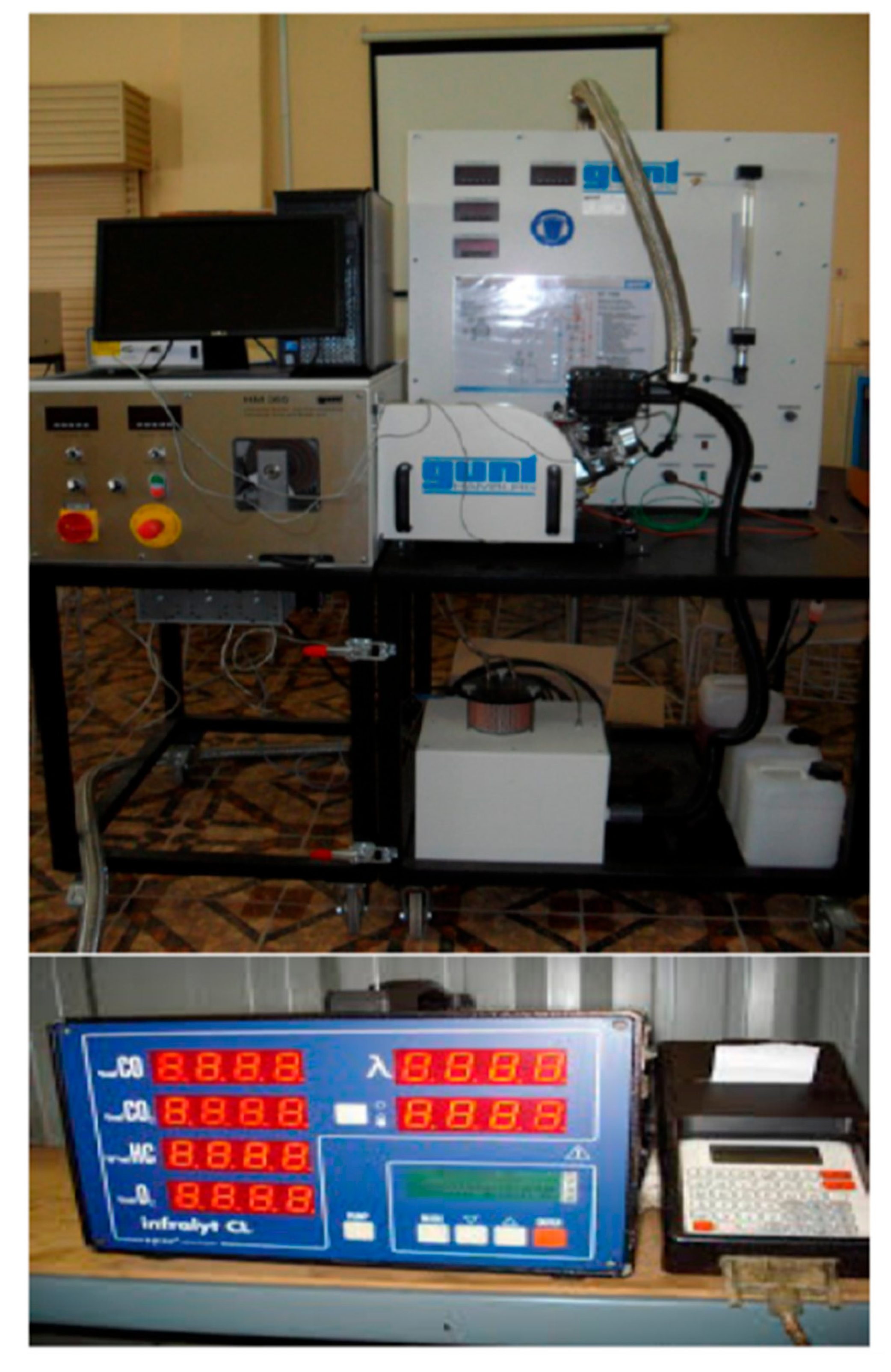
The experiments of this research, which are explained in this section, were applied to evaluate different types of biofuels for desalinations. The biofuels were examined through measuring the amount of energy/heat recovered and emissions. The experiments included a couple of measurements: The energy recovered from the combustion engine and the exhaust emissions, together with the emission amounts and types. There were two different experimental setups applied in the research, as shown in Figure 1: Combustion engine and exhaust gas analyzer. The combustion engine is a four-stroke gasoline engine with an air-cooled system. Full specifications of the engine are summarized in Table 1. The engine was connected with related sensors and auxiliary devices/instruments to control and measure the exhaust gas temperature at different engine speeds; in particular, the temperature was measured via thermocouple and the engine speed was controlled and measured via a dynamometer. On the other hand, the quantities and types of the exhaust emissions from the engine were measured via an exhaust gas analyzer from a kind of Infralyt CL. The analyzer was connected with the engine’s exhaust tail system. The exhaust gas analyzer operated with a power consumption of maximum 45 VA and heating range of 0–130 °C. The complete specifications of the exhaust gas analyzer are summarized in Table 1. The analyzer was capable of measuring carbon monoxide, carbon dioxide, and unburned hydrocarbons. The gas analyzer errors for emission measurements were evaluated and calibrated before measurements took place. It was calculated to be in the level ±2%. The accuracy of temperature sensor was about +/−1 °C. In addition, other sensor errors were calculated and found in satisfactory limits. For the measurements’ reproducibility, the measurements were almost repeated 3 times and found matching in the range 90–95%, while the standard deviation (SD) was almost from ±0.5% to ±0.1% SD.
The biofuels applied in the research were in the form of dual and ternary mixtures. Eight different biofuel blends were applied in the combustion engine as energy sources. Each blend was prepared and mixed at different rates and types to form one blended biofuel; then each blend was applied into the engine for evaluation. The eight different types of biofuel blends included dual and ternary issues and were prepared by mixing 93% gasoline with 7% bioethanol to form a bioethanol–gasoline blend (denoted as E). The second blend was prepared by mixing 93% gasoline with 7% biomethanol to form a gasoline–biomethanol blend (denoted as M). The third blend was prepared by mixing 93% gasoline with 7% n-butanol to form gasoline–n-butanol (denoted as nB). The fourth blend was prepared by mixing 93% gasoline and 7% iso-butanol to form a gasoline–isobutanol blend (denoted as iB). The fifth blend was prepared by mixing 93% gasoline with 7% bio-acetone to form a gasoline–bio-acetone blend (denoted as AC). These were five different types of dual blended issues. Additionally, three different types of ternary blended issues were prepared; the first one was prepared by mixing 93% gasoline with 7% bioethanol/biomethanol to form gasoline–bioethanol–biomethanol blended fuel (denoted as EM). In the second one, 93% gasoline was mixed with 7% n-butanol/isobutanol to form a gasoline–n-butanol–isobutanol blend (denoted as niB). In the last blend, 93% gasoline was mixed with 7% bioethanol/isobutanol to form a gasoline–bioethanol–isobutanol blend (denoted as iBE). It is worth noting that all blends included 7% biofuel (in dual or ternary issues) and 93% gasoline. The reasons for using such rates were the high costs of biofuels and that little of them would give the desired results. Further, such low biofuel rates did not require modifying the engine working conditions; however, adjustments had to be carried out in the engines in case of a biofuel blend ratio more than 10%.
3. Results and Discussions
The discussions and results of biofuel mixtures were presented here for the eight different types of dual and ternary blend issues. Comparisons between the different blends were carried out and the most suitable blend(s) was/were presented in terms of the least pollution and the highest energy recovered for desalination. Discussions regarding fuel burn, performance, and flame structure were briefly covered (without detail) as this requires independent work. Comparisons were carried out between the eight different blends in terms of exhaust gas temperature and emissions of CO, CO2, and UHC. The comparisons were applied at three different speeds (2500, 3000, and 3500 r/min), which represented low, medium, and high levels. The most appropriate engine speed(s) was/were also investigated and recommended, as obtainable afterwards. The emission results were presented primarily and compared; then, exhaust gas temperatures were introduced and compared for different speeds of engine and dissimilar biofuels.
Figure 2 shows carbon monoxide (CO) for gasoline–bioethanol (E), gasoline–biomethanol (M), gasoline–n-butanol (nB), gasoline–isobutanol (iB), and gasoline–bio-acetone (AC) dual blends at three different speeds (2500, 3000, and 3500 r/min); conventional gasoline (G) was the reference/baseline in the figure. As seen, diverse CO emission results were shown for the three different speeds. At a high speed (3500 r/min), for example, the lowest CO was shown by M, followed by AC; but at low and medium speeds, AC introduced the lowest CO emission. On the other hand, the greatest CO was shown by nB, followed by iB at both medium- and high-speed conditions (3000 and 3500 r/min). Further, M showed the greatest at low speed. Furthermore, all biofuel blends introduced lower CO than the G fuel at a low speed; however, at both medium and high speeds, both nB and iB showed higher emission levels than the G fuel; while both nB and iB introduced very low CO levels at a low speed.
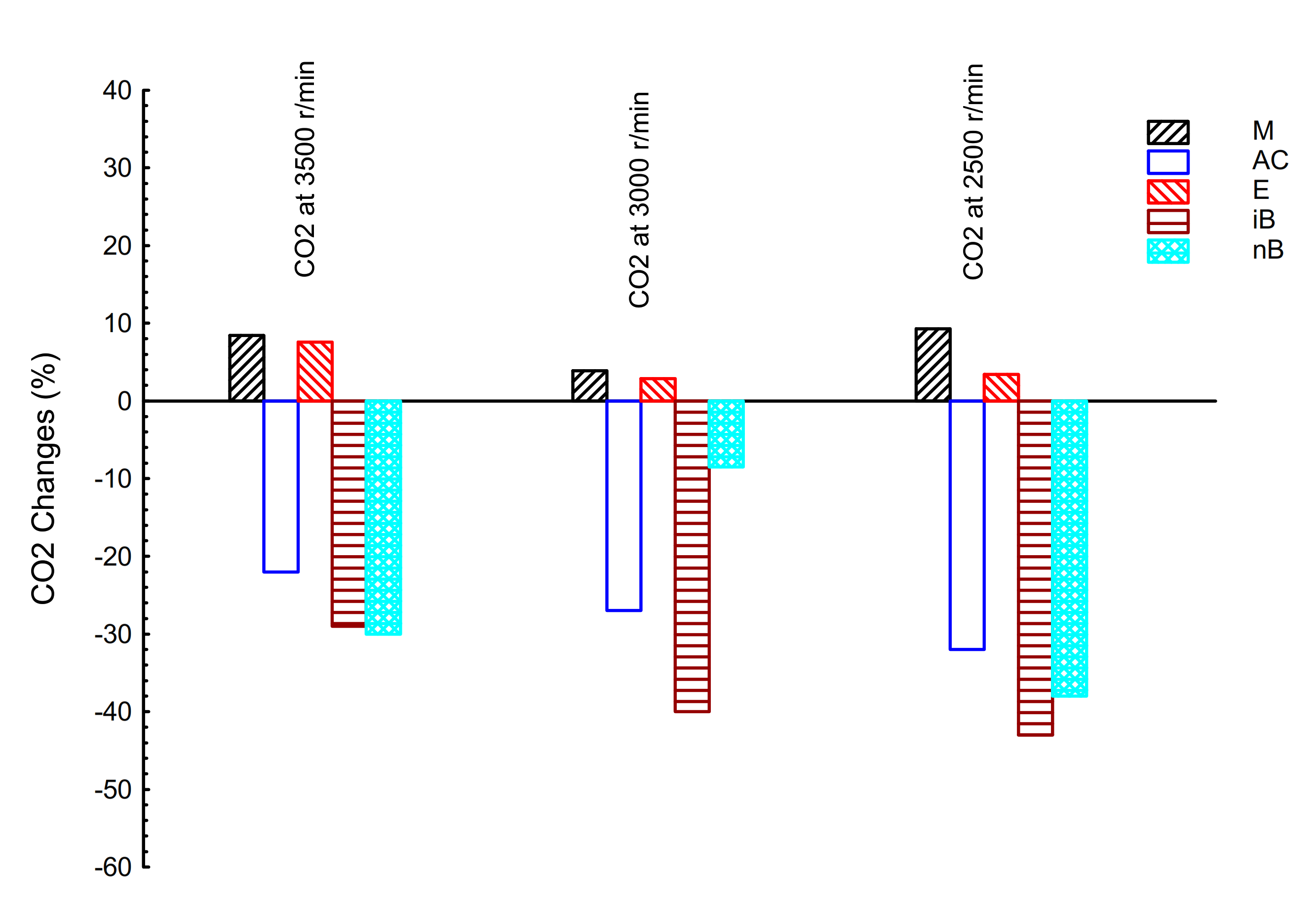
Figure 3 shows the unburned hydrocarbon (UHC) results for the five different dual blends at different speeds (low, medium, and high) and gasoline (the reference/baseline). As seen, iB showed greater UHC than the G fuel at a couple of speeds (medium and high); however, at low speed, the UHC emission of iB was very low. On the other hand, all other blends introduced lower UHC emissions than the G fuel in different levels via the three speeds. The lowest UHC was shown by M, nB, and AC at high, medium, and low speeds, respectively. The carbon dioxide (CO2) results are presented in Figure 4. As seen, both E and M showed greater CO2 levels than the G fuel at all speeds; however, AC, nB, and iB showed lower CO2 levels than the G fuel; the lowest CO2 were introduced via nB and iB. It is imperative to underline that CO2 is a greenhouse gas and some researches considered it a non-emission gas. However, it effects the environment in terms of warming of the globe and acid rain.
From Figure 2, Figure 3 and Figure 4, the emission results of the five blends are varied significantly with the engine speeds. The UHC of iB was lower than the G fuel at low speed; however, it was greater than the G at medium and/or high speeds. Additionally, both iB and nB showed lower CO levels than the G fuel at low speed, but they showed dissimilar styles at medium or high speeds. Such diverse trends at different speeds may be attributed to the air/fuel (AF) ratio, which is varied meaningfully with the engine speed; at a certain speed (low, medium, or high), the AF may match the stoichiometric AF conditions and, thus, low CO and UHC emissions would be obtained. By changing the engine speed from the stoichiometric condition, high CO and UHC emissions were established. Additionally, the fuel properties played a strong effect on trends, as shown in Table 2, and this is discussed later.
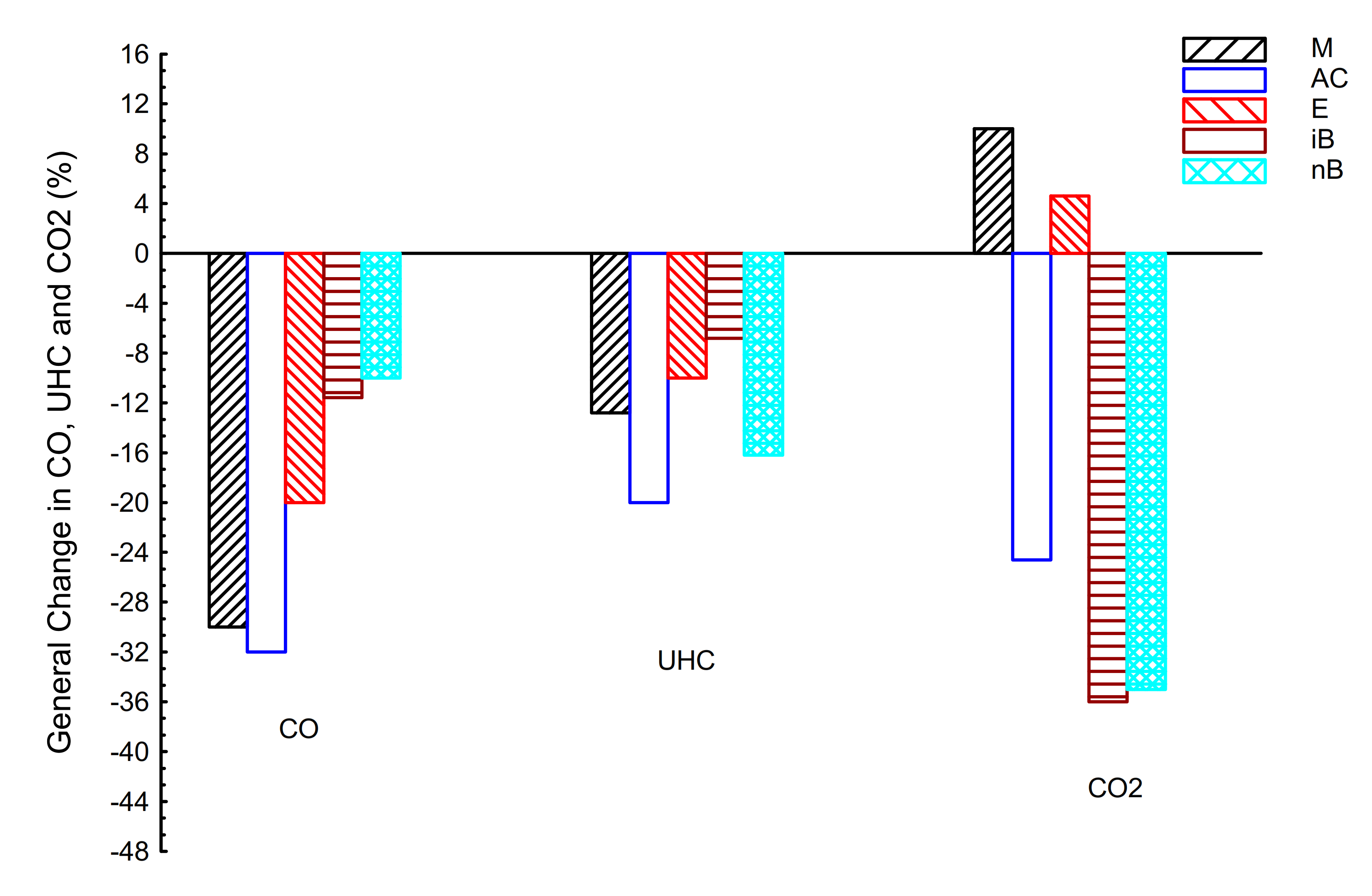
Figure 5 shows the comparisons of CO, CO2, and UHC emissions for the five different dual blends in average base among different speeds; gasoline is shown as the reference/baseline. The idea behind presenting such average results is that the average results were preferred as a simple comparison of different fuels to acquaint with the best one; however, results in different speeds, as shown early, could not easily provide such a conclusion. As shown in Figure 5, the lowest CO was introduced by AC, followed by M. Further, the CO emissions of both AC and M were very close, while other blends showed higher CO than those of AC and M; but all of them (M and AC) showed lower CO than the G fuel. In particular, the CO emissions for AC, M, E, iB, and nB were, respectively, about −32%, −30%, −20%, −11.6%, and −10%, compared to G fuel. The CO2 showed different trends from the CO emissions, where the lowest CO2 was shown by iB and the greatest value was shown by M. The CO2 emissions for iB, nB, AC, E, and M were, respectively, about −36%, −35%, −24.6%, 4.6%, and 10%, compared to G fuel. As seen, the M and E were the only blends that introduced greater CO2 values than the G fuel; however, AC, nB, and iB introduced lower CO2 levels than the G fuel. Concerning UHC emissions, the lowest UHC was shown by AC and the greatest was shown by iB. The UHC emissions for AC, nB, M, E, and iB were, respectively, about −20%, −16.2%, −12.8%, −10%, and −6.8%, compared to G fuel. The explanations of such emission results are introduced next.
The reasons for such emission results may refer to the following issues. Firstly, the blends were partially self-oxidized fuels because of containing oxygen in the structures, as shown in Table 2. The oxygen without doubt improved the combustion and, consequently, the emissions of CO and UHC. Secondary, the blends had a high heat of vaporizations, which enhanced the intake air for combustion (volumetric efficiency). Thirdly, the blends due to their low boiling conditions (as shown in Table 2) were vaporized and combusted very fast. Fourthly, the blends were combusted generally under very leaning conditions due to their low stoichiometric A/F ratios, compared to gasoline (see Table 2); such leaning conditions improved the combustion and reduced the CO and UHC emissions. On the other hand, the reason for lower CO and UHC emissions for AC, compared to other blends as well as G fuel, was that bio-acetone had the highest saturation pressure among all fuels; such great pressure increased the intake air and, in turn, extra lean combustion. On the other hand, the CO2 levels referred to the fuel complete combustion and carbon content in the biofuel. The M and E introduced the greatest CO2 due to their mostly complete combustion. The iB and nB showed low CO2 due to their somewhat high CO and UHC emissions. The reasons for CO2 of AC are be afforded later.
Table 3 shows the comparisons of CO, CO2, and UHC emissions for different dual and ternary blends in the average base among different speeds; gasoline is the reference/baseline. In this figure, three different biofuels in ternary blend issues were investigated and compared with the dual blends (introduced early in Figure 5). The ternary blends were intended for investigating and comparing more biofuels for the desalination process. As shown in Table 3, the ternary blends displayed reasonable values for all emissions. In detail, the CO emissions for EM, niB, and iBE were about −21%, −5%, and −14%, respectively, compared to G fuel. The CO2 emissions for EM, niB, and iBE were about 6.3%, −18%, and −14%, respectively, compared to G fuel. The UHC emissions for EM, niB, and iBE were about −18%, −14.5%, and −14%, respectively, compared to G fuel. In conclusion, ternary blends introduced moderate to high levels of emissions among all dual blended ones. Further, the niB showed the greatest CO and EM showed very high CO2 among all blends. Additionally, the UHC emissions of EM, niB, and iBE were moderate between all blends. Regarding the dual blends, some blends showed improved results and others showed the worst emissions, compared to ternary blends. In particular, AC dual blends showed better CO and UHC; but M showed worse CO2 than the ternary blends. In conclusion, to obtain low emissions of CO, CO2, and UHC, dual blended fuels (specific ones) were recommended over the ternary blends. The reason of such results may refer to the mixing conditions of ternary biofuel blends, e.g., a separation problem of one biofuel from another in the blend, which led to incomplete combustions and, in turn, high emissions. In addition, ternary blends may exceedingly prerequisite engine tuning/adjustment conditions compared to the dual ones. Additionally, the AC presented the best results because it seemed the most well-matched biofuel blend among all blends.
After evaluating and comparing the emissions of different blends, investigating heat recovering for desalination was carried out for the different blends, as follows. Figure 6 shows the exhaust gas temperature (EGT) for different dual blends at the three engine speeds; gasoline is the reference/baseline. As seen, the lowest EGT was shown by both nB and iB at all speeds, while the greatest EGT was shown by AC at a couple of speeds (low and high); at a medium speed, M introduces the greatest EGT value. Additionally, all blends (except for AC) showed lower EGT levels than the G fuel at a low speed. Further, both nB and iB introduced lower EGTs than the G at all speeds.
Figure 7 shows the exhaust gas temperature for the different dual blends in average principle; gasoline is the reference/baseline. From the figure, it is easy/relaxed to compare and highlight the best blend(s) for the EGT. As seen, the EGTs of different fuels were about 0.83%, 2.14%, 0.65%, −0.43%, and −5.3% for M, AC, E, iB, and nB, respectively, compared to G fuel. From these results, it was seen that the greatest EGT was introduced by AC, followed by M and E; however, the lowest EGT was shown by nB, followed by iB. Further, both nB and iB showed lower EGTs than the G fuel. A comparison of the EGTs of dual and ternary blends was carried out, as shown in Figure 8, in average base within different speeds; gasoline was the reference/baseline in the figure. As seen, all ternary blends (EM, niB, and iBE) introduced lower EGTs than the G fuel. Further, all blends (dual and ternary) provided lower EGTs than the G fuel, except for E, M, and AC dual blends. From these results, one may conclude that ternary blends are not recommended for the heat recovery process. Taking the emissions into consideration, the ternary mixed biofuels are not the best choice for desalination process.
In the results overview, ternary blends are unsuitable for desalinations since their EGT was very low in value (even lower than the G fuel). The dual blends nB and iB provided the same outcomes as the ternary blends (lower EGTs than the G fuel). The recommended blends for EGTs were the M, E, and AC dual blends. The best was the AC blend as it displayed greater EGT than M and E by about 1.31% and 1.49%, respectively. Concerning emissions, all blends showed lower emissions than the G fuel in different magnitudes (except for CO2 of E, M, and EM). In conclusion, AC was the best recommended one for both heat recovery and emissions of the desalination process. In addition, both E and M were recommended subsequently due to their high heat recovery and reasonable emissions (CO and UHC). All other blends (nB, iB, niB, iBE, and EM) were not highly recommended due to their low heat recovery (lower than the G fuel); however, they could provide acceptable emissions.
4. Conclusions
Desalination using fossil fuels is still the most considered approach among desalinations using alternative fuels worldwide. However, it struggles with some problems, including high pollutions, high energy consumption, and using non-renewable/depleted fuels. In this study, solutions to these struggles were proposed through applying renewable/biofuel blends in combustion engines, and then taking advantage of the engine lost energy for desalinations. In addition, using biofuels reduces the dependence on fossil fuels and decreases emissions. Ternary and dual blended biofuels were considered and compared, including gasoline/n-butanol (nB), gasoline/isobutanol (iB), gasoline/bioethanol (E), gasoline/biomethanol (M), gasoline/bio-acetone (AC), gasoline/n-butanol/isobutanol (niB), gasoline/bioethanol/isobutanol (iBE), and gasoline/bioethanol/biomethanol (EM) blends. The pollutants and energy recovered for each blend were investigated and compared with each other as well as with conventional gasoline; the results revealed that ternary blends (iBE, niB, and EM) were unsuitable for desalinations. Additionally, dual nB and iB blends showed lower heat recovery than the fossil gasoline. All blends showed lower emissions (CO and UHC) than the fossil gasoline fuel. The recommended blends for heat recovery were the M, E, and AC dual blends. However, E and M introduced high CO2 greenhouse gas. The superlative recommended blend in terms of greater heat recovery and lower emissions was AC among all blends.
Funding
This research was funded by Taif University researchers supporting project number (TURSP–2020/40), Taif University, Taif, Saudi Arabia. The APC was funded by Taif University researchers supporting project number (TURSP–2020/40), Taif University, Taif, Saudi Arabia.
Acknowledgments
This work was supported by Taif University researchers supporting project number (TURSP–2020/40), Taif University, Taif, Saudi Arabia.
Conflicts of Interest
The author declares no conflict of interest.
References
- Gleick, P.H. The World’s Water 2006–2007: The Biennial Report on Freshwater Resources; Island Press: Washington, DC, USA, 2006. [Google Scholar]
- Elsaid, K.; Kamil, M.; Sayed, E.T.; Abdelkareem, M.A.; Wilberforce, T.; Olabi, A. Environmental impact of desalination technologies: A review. Sci. Total Environ. 2020, 748, 141528. [Google Scholar] [CrossRef] [PubMed]
- Ng, K.C.; Shahzad, M.W. Sustainable desalination using ocean thermocline energy. Renew. Sustain. Energy Rev. 2018, 82, 240–246. [Google Scholar] [CrossRef]
- Alnajdi, O.; Calautit, J.K.; Wu, Y. Development of a multi-criteria decision making approach for sustainable seawater desalination technologies of medium and large-scale plants: A case study for Saudi Arabia’s vision 2030. Energy Procedia 2019, 158, 4274–4279. [Google Scholar] [CrossRef]
- Gleick, P.H.; Allen, L.; Cohen, M.J.; Cooley, H.; Christian–Smith, J.; Heberger, M.; Morrison, J.; Palaniappan, M.; Schulte, P. The World’s Water: The Biennial Report on Freshwater Resources; Island Press: Washington, DC, USA, 2012; Volume 7. [Google Scholar]
- Jones, E.; Qadir, M.; Van Vliet, M.T.; Smakhtin, V.; Kang, S.-M. The state of desalination and brine production: A global outlook. Sci. Total Environ. 2019, 657, 1343–1356. [Google Scholar] [CrossRef]
- Heck, N.; Lykkebo Petersen, K.; Potts, D.C.; Haddad, B.; Paytan, A. Predictors of coastal stakeholders’ knowledge about seawater desalination impacts onmarine ecosystems. Sci. Total Environ. 2018, 639, 785–792. [Google Scholar] [CrossRef] [Green Version]
- Panagopoulos, A.; Haralambous, K.-J.J.; Loizidou, M. Desalination brine disposal methods and treatment technologies—A review. Sci. Total Environ. 2019, 693, 133545. [Google Scholar] [CrossRef]
- Ang, W.L.; Mohammad, A.W.; Johnson, D.; Hilal, N. Unlocking the application potential of forward osmosis through integrated/hybrid process. Sci. Total Environ. 2020, 706, 136047. [Google Scholar] [CrossRef] [Green Version]
- Elsaid, K.; Sayed, E.T.; Abdelkareem, M.A.; Baroutaji, A.; Olabi, A. Environmental impact of desalination processes: Mitigation and control strategies. Sci. Total Environ. 2020, 740, 140125. [Google Scholar] [CrossRef]
- Werner, M.; Schäfer, A.I. Social aspects of a solar–powered desalination unit for remote Australian communities. Desalination 2007, 203, 375–393. [Google Scholar] [CrossRef]
- McGrath, C. Renewable Desalination Market Analysis in Oceania, South Africa, Middle East & North Africa; Aquamarine Power: Edinburgh, UK, 2011. [Google Scholar]
- Malik, M.A.S.; Tiwari, N.; Kumar, A.; Sodha, M.S. Active and Passive Solar Distillation: A Review; Pergamon Press: Oxford, UK, 1982. [Google Scholar]
- Aayush, K. VarunSolar stills: A review. Renew. Sustain. Energy Rev. 2010, 14, 446–453. [Google Scholar]
- Tiwari Singh, G.N.; Tripathi Rajesh, H.N. Present status of solar distillation. Sol. Energy 2003, 75, 367–373. [Google Scholar] [CrossRef]
- Murugavel, K.K.; Chockalingam, K.; Srithar, K. Progresses in improving the effectiveness of the single basin passive solar still. Desalination 2008, 220, 677–686. [Google Scholar] [CrossRef]
- Sampathkumar, K.; Arjunan, T.V.; Pitchandi, P.; Senthilkumar, P. Active solar distillation—A detailed review. Renew. Sustain. Energy Rev. 2010, 14, 1503–1526. [Google Scholar] [CrossRef]
- Velmurugan, V.; Srithar, K. Performance analysis of solar stills based on various factors affecting the productivity—A review. Renew. Sustain. Energy Rev. 2011, 15, 1294–1304. [Google Scholar] [CrossRef]
- Kabeel, A.; El-Agouz, S. Review of researches and developments on solar stills. Desalination 2011, 276, 1–12. [Google Scholar] [CrossRef]
- Alsehli, M.; Saleh, B.; Elfasakhany, A.; Aly, A.A.; Bassuoni, M.M. Experimental study of a novel solar multi–effect distillation unit using alternate storage tanks. J. Water Reuse Desalin. 2020, 10, 120–132. [Google Scholar] [CrossRef]
- Elfasakhany, A. Performance assessment and productivity of a simple–type solar still integrated with nanocomposite energy storage system. Appl. Energy 2016, 183, 399–407. [Google Scholar] [CrossRef]
- Elfasakhany, A. Modeling of Pulverised Wood Flames. Ph.D. Thesis, Lund University, Fluid Mechanics Department, Lund, Sweden, 2005. [Google Scholar]
- Elfasakhany, A.; Tao, L.; Espenas, B.; Larfeldt, J.; Bai, X.S. Pulverised Wood Combustion in a Vertical Furnace: Experimental and Computational Analyses. Appl. Energy 2013, 112, 454–464. [Google Scholar] [CrossRef]
- Elfasakhany, A. Gasoline engine fueled with bioethanol–bio–acetone–gasoline blends: Performance and emissions exploration. Fuel 2020, 274, 117825. [Google Scholar] [CrossRef]
- Elfasakhany, A. Experimental investigation on SI engine using gasoline and a hybrid iso–butanol/gasoline fuel. Energy Convers. Manag. 2015, 95, 398–405. [Google Scholar] [CrossRef]
- Shahzad, M.W.; Burhan, M.; Ang, L.; Ng, K.C. Energy-water-environment nexus underpinning future desalination sustainability. Desalination 2017, 413, 52–64. [Google Scholar] [CrossRef]
- Shahzad, M.W.; Burhan, M.; Son, H.S.; Oh, S.J.; Ng, K.C. Desalination processes evaluation at common platform: A universal performance ratio (UPR) method. Appl. Therm. Eng. 2018, 134, 62–67. [Google Scholar] [CrossRef] [Green Version]
- Ng, K.C.; Shahzad, M.W.; Son, H.S.; Hamed, O.A. An exergy approach to efficiency evaluation of desalination. Appl. Phys. Lett. 2017, 110, 184101. [Google Scholar] [CrossRef] [Green Version]
- Shahzad, M.W.; Burhan, M.; Ng, K.C. A standard primary energy approach for comparing desalination processes. NPJ Clean Water 2019, 2, 1–7. [Google Scholar] [CrossRef] [Green Version]
- Shahzad, M.W.; Burhan, M.; Ybyraiymkul, D.; Ng, K.C. Desalination Processes’ Efficiency and Future Roadmap. Entropy 2019, 21, 84. [Google Scholar] [CrossRef] [Green Version]
- Gude, V.G. Thermal desalination of ballast water using onboard waste heat in marine industry. Int. J. Energy Res. 2019, 43, 6026–6037. [Google Scholar] [CrossRef]
- Ouyang, T.; Su, Z.; Gao, B.; Pan, M.; Chen, N.; Huang, H. Design and modeling of marine diesel engine multistage waste heat recovery system integrated with flue-gas desulfurization. Energy Convers. Manag. 2019, 196, 1353–1368. [Google Scholar] [CrossRef]
- Lion, S.; Vlaskos, I.; Taccani, R. A review of emissions reduction technologies for low and medium speed marine Diesel engines and their potential for waste heat recovery. Energy Convers. Manag. 2020, 207, 112553. [Google Scholar] [CrossRef]
- Lion, S.; Michos, C.N.; Vlaskos, I.; Rouaud, C.; Taccani, R. A review of waste heat recovery and Organic Rankine Cycles (ORC) in on-off highway vehicle Heavy Duty Diesel Engine applications. Renew. Sustain. Energy Rev. 2017, 79, 691–708. [Google Scholar] [CrossRef]
- Seyedkavoosi, S.; Javan, S.; Kota, K. Exergy-based optimization of an organic Rankine cycle (ORC) for waste heat recovery from an internal combustion engine (ICE). Appl. Therm. Eng. 2017, 126, 447–457. [Google Scholar] [CrossRef]
- Salimi, M.; Amidpour, M. Modeling, simulation, parametric study and economic assessment of reciprocating internal combustion engine integrated with multi-effect desalination unit. Energy Convers. Manag. 2017, 138, 299–311. [Google Scholar] [CrossRef]
- Chintala, V.; Kumar, S.; Pandey, J.K. A technical review on waste heat recovery from compression ignition engines using organic Rankine cycle. Renew. Sustain. Energy Rev. 2018, 81, 493–509. [Google Scholar] [CrossRef]
- Shafieian, A.; Khiadani, M. A multipurpose desalination, cooling, and air-conditioning system powered by waste heat recovery from diesel exhaust fumes and cooling water. Case Stud. Therm. Eng. 2020, 21, 100702. [Google Scholar] [CrossRef]
- Yang, F.; Cho, H.; Zhang, H.; Zhang, J. Thermoeconomic multi-objective optimization of a dual loop organic Rankine cycle (ORC) for CNG engine waste heat recovery. Appl. Energy 2017, 205, 1100–1118. [Google Scholar] [CrossRef]
- Asadi, A.; Meratizaman, M.; Hosseinjani, A.A. Feasibility study of small-scale gas engine integrated with innovative net-zero water desiccant cooling system and single-effect thermal desalination unit. Int. J. Refrig. 2020, 119, 276–293. [Google Scholar] [CrossRef]
- Elfasakhany, A. Investigation on performance and emissions characteristics of an internal combustion engine fuelled with petroleum gasoline and a hybrid methanol–gasoline fuel. Int. J. Eng. Tech. 2013, 13, 24–43. [Google Scholar]
- Elfasakhany, A. The Effects of Ethanol–Gasoline Blends on Performance and Exhaust Emission Characteristics of Spark Ignition Engines. Int. J. Automot. Eng. 2014, 4, 608–620. [Google Scholar]
- Elfasakhany, A. Exhaust emissions and performance of ternary iso–butanol–bio–methanol–gasoline and n–butanol–bio–ethanol–gasoline fuel blends in spark–ignition engines: Assessment and comparison. Energy 2018, 158, 830–844. [Google Scholar] [CrossRef]
- Gong, C.; Yi, L.; Zhang, Z.; Sun, J.; Liu, F. Assessment of ultra-lean burn characteristics for a stratified-charge direct-injection spark-ignition methanol engine under different high compression ratios. Appl. Energy 2020, 261, 114478. [Google Scholar] [CrossRef]
- Zhen, X.; Wang, Y. An overview of methanol as an internal combustion engine fuel. Renew. Sustain. Energy Rev. 2015, 52, 477–493. [Google Scholar] [CrossRef]
- Gong, C.; Li, Z.; Yi, L.; Liu, F. Comparative study on combustion and emissions between methanol port-injection engine and methanol direct-injection engine with H2-enriched port-injection under lean-burn conditions. Energy Convers. Manag. 2019, 200, 112096. [Google Scholar] [CrossRef]
- Gong, C.; Li, Z.; Chen, Y.; Liu, J.; Liu, F.; Han, Y. Influence of ignition timing on combustion and emissions of a spark–ignition methanol engine with added hydrogen under lean-burn conditions. Fuel 2019, 235, 227–238. [Google Scholar] [CrossRef]
- Gong, C.; Li, Z.; Yi, L.; Huang, K.; Liu, F. Research on the performance of a hydrogen/methanol dual-injection assisted spark–ignition engine using late-injection strategy for methanol. Fuel 2020, 260, 116403. [Google Scholar] [CrossRef]
- Elfasakhany, A.; Mahrous, A.F. Performance and emissions assessment of n–butanol–methanol–gasoline blends as a fuel in spark–ignition engines. Alex. Eng. J. 2016, 55, 3015–3024. [Google Scholar] [CrossRef] [Green Version]
- Elfasakhany, A. Investigations on the effects of ethanol–methanol–gasoline blends in a spark-ignition engine: Performance and emissions analysis. Eng. Sci. Technol. Int. J. 2015, 18, 713–719. [Google Scholar] [CrossRef] [Green Version]
- Elfasakhany, A. Engine performance evaluation and pollutant emissions analysis using ternary bio-ethanol–iso-butanol–gasoline blends in gasoline engines. J. Clean. Prod. 2016, 139, 1057–1067. [Google Scholar] [CrossRef]
- Elfasakhany, A. Experimental study of dual n-butanol and iso-butanol additives on spark-ignition engine performance and emissions. Fuel 2016, 163, 166–174. [Google Scholar] [CrossRef]
- Elfasakhany, A. Experimental study on emissions and performance of an internal combustion engine fueled with gasoline and gasoline/n-butanol blends. Energy Convers. Manag. 2014, 88, 277–283. [Google Scholar] [CrossRef]
- Elfasakhany, A. Performance and emissions analysis on using acetone–gasoline fuel blends in spark-ignition engine. Eng. Sci. Technol. Int. J. 2016, 19, 1224–1232. [Google Scholar] [CrossRef] [Green Version]
- Elfasakhany, A. Performance and emissions of spark–ignition engine using ethanol–methanol–gasoline, n–butanol–iso–butanol–gasoline and iso–butanol–ethanol–gasoline blends: A comparative study. Eng. Sci. Technol. 2016, 19, 2053–2059. [Google Scholar] [CrossRef] [Green Version]
- Elfasakhany, A. Investigations on performance and pollutant emissions of spark–ignition engines fueled with n–butanol–, iso–butanol–, ethanol–, methanol–, and acetone–gasoline blends: A comparative study. Renew. Sustain. Energy Rev. 2017, 71, 404–413. [Google Scholar] [CrossRef]
- Elfasakhany, A. Biofuels in Automobiles: Advantages and Disadvantages: A Review. Curr. Altern. Energy 2019, 3, 1–7. [Google Scholar] [CrossRef]
- Elfasakhany, A. Alcohols as Fuels in Spark Ignition Engines: Second Blended Generation; LAMBERT Academic Publishing: Saarbrücken, Germany, 2017; ISBN 978–3–659–97691–9. [Google Scholar]
- Elfasakhany, A. Benefits and Drawbacks on the Use Biofuels in Spark Ignition Engines; LAMBERT Academic Publishing: Beau-Bassin, Mauritius, 2017; ISBN 978–620–2–05720–2. [Google Scholar]
Figure 1.
Photo of experimental set-up for engine and gas analyzer.

Figure 2.
Carbon monoxide (CO) for gasoline–bioethanol (E), gasoline–biomethanol (M), gasoline–n-butanol (nB), gasoline-iso-butanol (iB), and gasoline–bio-acetone (AC) dual blends at three different speeds (2500, 3000, and 3500 r/min); gasoline is the reference/baseline.
Figure 2.
Carbon monoxide (CO) for gasoline–bioethanol (E), gasoline–biomethanol (M), gasoline–n-butanol (nB), gasoline-iso-butanol (iB), and gasoline–bio-acetone (AC) dual blends at three different speeds (2500, 3000, and 3500 r/min); gasoline is the reference/baseline.

Figure 3.
Unburned hydrocarbon (UHC) for different dual blends at three different speeds. Captions are seen in Figure 2; gasoline is the reference/baseline.
Figure 3.
Unburned hydrocarbon (UHC) for different dual blends at three different speeds. Captions are seen in Figure 2; gasoline is the reference/baseline.

Figure 4.
Carbon dioxide (CO2) for different dual blends at three different speeds. Captions are seen in Figure 2; gasoline is the reference/baseline.
Figure 4.
Carbon dioxide (CO2) for different dual blends at three different speeds. Captions are seen in Figure 2; gasoline is the reference/baseline.

Figure 5.
Comparisons of CO, CO2, and UHC emissions for different dual blends in average base of different speeds. Captions are seen in Figure 2; gasoline is the reference/baseline.
Figure 5.
Comparisons of CO, CO2, and UHC emissions for different dual blends in average base of different speeds. Captions are seen in Figure 2; gasoline is the reference/baseline.

Figure 6.
Exhaust gas temperature (EGT) for different dual blends at three different speeds. Captions are seen in Figure 2; gasoline is the reference/baseline.
Figure 6.
Exhaust gas temperature (EGT) for different dual blends at three different speeds. Captions are seen in Figure 2; gasoline is the reference/baseline.

Figure 7.
Exhaust gas temperature (EGT) for different dual blends in average principle. Captions are seen in Figure 2; gasoline is the reference/baseline.
Figure 7.
Exhaust gas temperature (EGT) for different dual blends in average principle. Captions are seen in Figure 2; gasoline is the reference/baseline.

Figure 8.
Comparisons of exhaust gas temperature (EGT) for different dual and ternary blends in average base of different speeds. Captions are seen in Figure 2 and Figure 5; gasoline is the reference/baseline.


Table 1.
Gasoline engine and pollutant gas analyzer specifications.
| Engine Specifications | |
| Cylinder(s) | 1 |
| Valves | 2 |
| Bore (mm) | 65.1 |
| Stroke (mm) | 44.4 |
| Compression ratio | 7:1 |
| Displacement (cm3) | 147.7 |
| Maximum power (KW) | 1.5 |
| Weight (Kg) | 17 Kg |
| Type | Spark-ignition |
| Gas Analyzer Specifications | |
| Warm-up period | 10 min |
| Weight | 9 kg |
| Exhaust gas temperature | 5–45 °C |
| Measurement ranges | CO 0–10 vol.% |
| CO2 0–20 vol.% | |
| UHC 0–2000 ppm vol. (as C6H14) | |
| Voltage | 230 V (+10%/–15%) |
| Frequency | 50 +/−1 Hz |
| Power consumption | Max. 45 VA |
| Range of apparatus heating | 0–130 °C, resolution ±1 °C |
| Property | Gasoline | Bioethanol | Biomethanol | Isobutanol | N-Butanol | Bio-Acetone |
|---|---|---|---|---|---|---|
| Chemical formula C3H6O | C8H15 | C2H5OH | CH3OH | C4H9OH | C4H9OH | C3H6O |
| Composition (C,H,O) % | 86, 14, 0 | 52, 13, 35 | 37.5, 12.5, 50 | 65, 13.5, 21.5 | 65, 13.5, 21.5 | 62, 10.5, 27.5 |
| Lower heating value (MJ/kg) | 43.5 | 27.0 | 20.1 | 33.3 | 33.1 | 29.6 |
| Heat of evaporation (kJ/kg) | 223.2 | 725.4 | 920.7 | 474.3 | 582 | 501.7 |
| Stoichiometric A/F ratio | 14.6 | 9.0 | 6.4 | 11.1 | 11.2 | 9.54 |
| Oxygen content, mass % | 0.0 | 34.7 | 49.9 | 21.6 | 21.6 | 27.6 |
| Density (kg/m3) | 760 | 790 | 796 | 802 | 810 | 791 |
| Sat. pressure at 38 °C (kPa) | 31 | 13.8 | 31.69 | 2.3 | 2.27 | 53.4 |
| Flash point (°C) | −40 | 21.1 | 11.1 | 28 | 35 | 17.8 |
| Auto–ignition temp. (°C) | 420 | 434 | 470 | 415 | 385 | 560 |
| Boiling point (°C) | 25–215 | 78.4 | 64.5 | 108 | 117.7 | 56.1 |
| Solubility in water | <0.1 | Fully miscible | Fully miscible | 10.6 | 7.7 | Miscible |
Table 3.
Comparing emissions of dual and ternary biofuel blends in average rules (%).
| Biofuel Blends | CO | UHC | CO2 | |
|---|---|---|---|---|
| Emissions | ||||
| M | −30 | −12.8 | 10 | |
| AC | −32 | −20 | −24.6 | |
| E | −20 | −10 | 4.6 | |
| iB | −11.6 | −6.8 | −36 | |
| nB | −10 | −16.2 | −35 | |
| niB | −5 | −13.5 | −18 | |
| iBE | −14 | −14 | −14 | |
| EM | −21 | −18 | 6.3 | |
The reference is the value for conventional gasoline (considered as zero).
Publisher’s Note: MDPI stays neutral with regard to jurisdictional claims in published maps and institutional affiliations. |
© 2020 by the author. Licensee MDPI, Basel, Switzerland. This article is an open access article distributed under the terms and conditions of the Creative Commons Attribution (CC BY) license (http://creativecommons.org/licenses/by/4.0/).
Share and Cite
MDPI and ACS Style
Elfasakhany, A. Dual and Ternary Biofuel Blends for Desalination Process: Emissions and Heat Recovered Assessment. Energies 2021, 14, 61. https://0-doi-org.brum.beds.ac.uk/10.3390/en14010061
AMA Style
Elfasakhany A. Dual and Ternary Biofuel Blends for Desalination Process: Emissions and Heat Recovered Assessment. Energies. 2021; 14(1):61. https://0-doi-org.brum.beds.ac.uk/10.3390/en14010061
Chicago/Turabian StyleElfasakhany, Ashraf. 2021. "Dual and Ternary Biofuel Blends for Desalination Process: Emissions and Heat Recovered Assessment" Energies 14, no. 1: 61. https://0-doi-org.brum.beds.ac.uk/10.3390/en14010061
Note that from the first issue of 2016, this journal uses article numbers instead of page numbers. See further details here.