
Energy Community Flexibility Solutions to Improve Users’ Wellbeing


1
Department of Electrical and Computer Engineering, NOVA School of Science and Technology (FCT NOVA), 2829-516 Caparica, Portugal
2
Center of Technology and Systems (CTS)—UNINOVA, 2829-516 Caparica, Portugal
*
Author to whom correspondence should be addressed.
Energies 2021, 14(12), 3403; https://0-doi-org.brum.beds.ac.uk/10.3390/en14123403
Submission received: 20 April 2021
/
Revised: 31 May 2021
/
Accepted: 4 June 2021
/
Published: 9 June 2021
(This article belongs to the Special Issue Power Systems Connectivity and Resiliency: Modeling, Simulation and Analysis)
Abstract
:Energy communities, mostly microgrid based, are a key stakeholder of modern electrical power grids. Operating a microgrid based energy community is a challenging topic due to the involved uncertainties, complexities and often conflicting objectives. The aim of this paper is to present a novel methodology demonstrating that energy community flexibility can contribute to each community member’s wellbeing when a grid fault occurs. A three-house energy community will be modelled considering as consumption sources non-controllable and controllable devices in each house. As power supply sources, PV systems installed in a community’s houses are considered, as well as the power obtained from main grid. Each house’s flexibility inside the community will be studied to improve the management of loads during a fault occurrence. Moreover, three different scenarios will be considered with different available power in the community. With these simulations, it was possible to understand that houses’ energy flexibility can be used under a fault situation, either to maintain the users’ wellbeing or to change the energy flow. Furthermore, energy flexibility can be used to create better energy price markets, to improve the resilience of the grid, or even to consider electrical vehicles’ connection to a community’s grid.
1. Introduction
Whenever there is a fault at any part of the electrical power grid (EPG), different levels of consequences will be generated for the entire grid [1]. Faults affecting only a small part of the EPG, with stress-free and fast resolution, do not imply a redirection of the energy flow through other transmission paths. However, catastrophic events may imply the isolation of other sections of the EPG’s, thus leading to overload due to load redistribution, and cascade failure [2,3,4].
Climate change and its negative impact on the environment are amongst the most pressing challenges for the planet. Most of the produced energy (70.1%) still comes from conventional energy sources including oil, coal, and gas with high pollution emissions [5]. According to the European Commission, energy production and heat generation from conventional fuels will be responsible for 54% of European Union greenhouse gas emissions by the year of 2017 [5]. Thus, renewable sources are seen as a solution, by policymakers and governments, to creating a more competitive and sustainable energy system and to mitigate the climate change effects [6]. In fact, European countries committed themselves to increase the share of energy consumption to 20% by 2020 and 32% by 2030 [5]. Despite some resistance to accepting some renewable energy related changes, promising approaches are emerging, of which a good example is the concept of energy communities (EnC). For the European Commission, EnC are characterized by citizens’ groups, social entrepreneurs, public authorities and community organizations that participate in the energy production, trading, distribution, and consumption of renewable energy [7,8].
Due to the renewable energy’s development and democratization related issues, citizens began to be considered as an active player in the system, usually addressed as prosumers. In general, a community is a social unit that has something in common, a group of users that can actively participate in the consumption and production of energy [9,10]. Energy communities are established by including energy conversion, transmission, and consumption on a community scale. Energy flow balancing, reducing peak load during peak hours, territorial energy planning, interconnection of different energy carriers or mitigation of environmental impacts are relevant items that EnC can cover under the energy context [11].
Energy planning issues and on-site supply potential are key elements that lead to an increased level of energy supply for communities [12]. Regarding EnC’s prosumers, and the possibility of managing their energy consumption and production, the concept of energy flexibility is an extremely important added value [13]. In a building, or in a community, flexible loads allow the redistribution of power throughout the day to meet different constrains and objectives [14].
A resilient engineering system is often regarded as a system with the ability to maintain its performance during an outage, providing reliability and adaptability. However, it can also be considered a robust system with resistance to disturbances and the ability to quickly recover after the outage. Considering the aforementioned constrains and the resilience definition, and using the EnC’s flexibility, the resilience of the supporting microgrid can be improved under fault conditions. Moreover, flexibility is directly related to the community and microgrid’s resilience, i.e., if the community’s flexibility increases, consequently the community will become more resilient, so flexibility forecasting [15] will be extremely useful in order to improve grid resilience.
Focusing on local energy communities, and considering that the term community refers to a group of users/houses (preferably net-zero energy communities, which are expected to be large scale deployed in the near future [16]) interconnected by a microgrid, the EnC approach followed in this paper is depicted in Figure 1. EnCs’ implementation intends to increase energy self-consumption ratios through demand response. The work presented in [17] is intended to ensure that most of the consumption occurs during the day (when PV plants are producing). The current paper explores the possibilities of using the community’s energy flexibility to maintain the users’ wellbeing when a fault occurs. Inside the community, each house is considered to have renewable energy production as well as flexible (controllable) consumption devices.
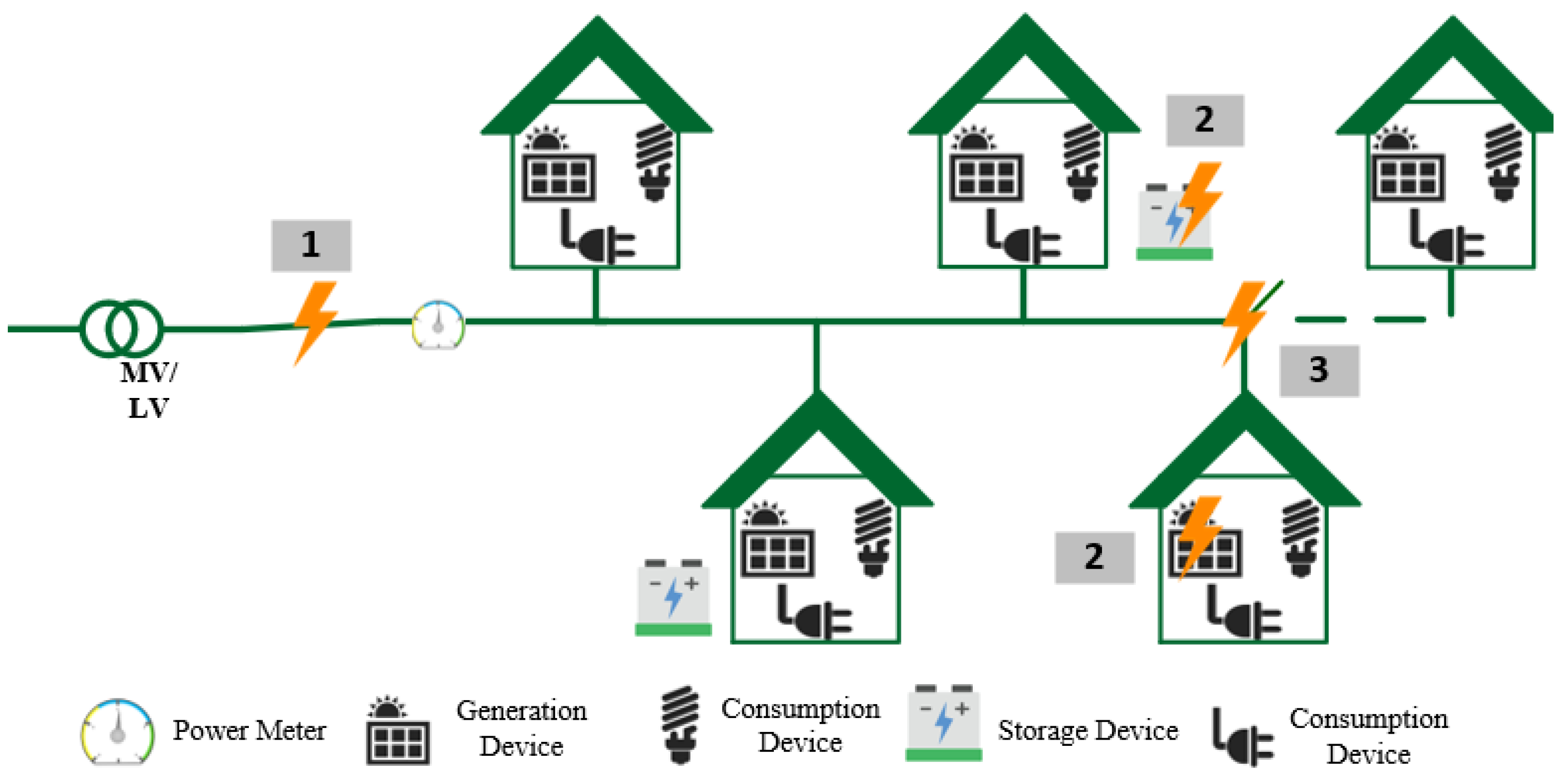
Considering this setup, where the EnC is part of a microgrid, different types of power failure faults can be considered. Figure 2 presents four distinct power failure conditions that can occur inside an EnC. The first (1) denotes two distinct situations: (1a) isolation of the whole community from the main grid in case of total outage, or (1b) power curtailment from the main grid to the community. The second (2) represents a storage or generation devices’ fault. This will decrease the available power, affecting community behavior. The last (3) denotes a cable fault inside the EnC microgrid. This power outage will isolate some community members that will act as a new, partial, isolated EnC needing to readapt their behavior.
This paper demonstrates that the usage of each EnC member’s energy flexibility will improve the EnC microgrid’s overall resilience and will contribute to the new body of knowledge. Appliances will be characterized using finite state machines combined with alternative load profile computation. This will allow better control of their operational cycle through better flexibility usage. For every power failure condition, a set of feasible scenarios are identified within the day (appliances’ earlier, mid, or later start), taking into account technical constraints, allowing each householder to become an active part of the solution without compromising their wellbeing.
During the following subsections, knowledge gaps are identified, namely how to use the EnC concept in order to maintain the users’ wellbeing through the home devices’ energy flexibility.
1.1. Background
Different types of energy communities are mentioned in the literature. Some of them consider net zero energy buildings (NZEBs) in their composition [18]; positive energy buildings (PEBs) [19]; regular houses with controllable devices and renewable energy production that are aggregated using their combined flexibility in the community [20]; prosumers; or even plain consumers [21].
Figure 3 illustrates the variety of distinct houses that can coexist inside an EnC. In the case of NZEB, the EU Energy Performance in Buildings Directive [22] defines them as “a building that has a very high energy performance and the nearly zero or very low amount of energy required should be covered to a very significant extent by energy from renewable sources, including energy from renewable sources produced on-site or nearby”. Normally, a period of one year is considered in order to cover the distinct meteorological conditions [23]. In line with Figure 3, if the global energy demand equals the amount of locally supplied energy, then one can have a net zero energy community (NZEC).
Following the NZEB technologies and solutions development, the concept has evolved towards positive energy buildings (PEB). When the exported energy from a building, during a pre-defined period of time, is higher than the imported energy, the building is called a positive-energy building (PEB) [24]. Also, as Figure 3 illustrates, a group of buildings that actively manage their energy consumption and the energy flow between them and the wider energy system, as well as presenting a positive annual energy balance [25], is called a positive energy block (PEBlock) or a positive energy district (PED) [26].
1.1.1. Energy Flexibility
Besides the PEBlock concept [27], it is important to deeply analyze the neighborhood/community flexibility level since reliability and resilience enhancement can be provided by the community flexibility level demand-side resources [28]. Furthermore, a PEBlock will be able to enhance its flexibility if different resources are exploited [29]. These resources are storage devices (allowing a shift in demand in real time), controllable household devices, or energy production devices.
The energy flexibility concept can be considered from different viewpoints. In [30], Reynders identifies five different focuses to consider flexibility: energy infrastructure, systems interaction with building, energy price, building performance, and electricity. For LeDréau energy flexibility represents the ability to change the energy usage from high to low price periods [31]. Hong considers energy flexibility as the time window maximization where the heat pumping operation time can be shifted without affecting comfort and hot water supply temperatures for the end-user [31]. Energy flexibility can be characterized as a static function at every time instant, however Junker proposed a methodology that characterizes it as a dynamic function allowing grid operators to control the demand through the use of penalty signals, for example price or CO2 emissions [14]. Penalty signals are often used as a way to characterize and use energy flexibility [14]. There are several approaches and methodologies to quantify energy flexibility already reported in the literature. In his review paper [30], Reynders presented a list of five different methodologies to quantify energy flexibility based on different approaches: (a) number of hours that energy consumption can be delayed or anticipated (temporal flexibility) [30]; (b) power increase or decrease, combined with how long these changes can be maintained (power flexibility) [31]; (c) combination of both temporal and power flexibility, together with energy flexibility [14]; (d) amount of energy that can be shifted at a specific moment and the respective cost compared to a base cost plan [32]; and (e) available storage capacity, storage efficiency, and the power shifting potential [33].
To demonstrate that the usage of each energy community member’s energy flexibility will improve the energy community microgrid’s resilience, both power and temporal flexibility will be considered. Considering the overall community’s energy flexibility in real time, the appliances’ working time can be adapted if necessary and the power consumption of each community’s user can be changed. Two important issues to take into account are the house’s energy management and the household devices to be considered. The work in [34] presents an efficient home energy management scheme that aims to reduce energy usage and monetary cost for smart grid communities. Also, Stephant uses game theory to model the preferences of each user and to build a mathematical framework where each user individually optimizes his power profile according to these preferences in order to improve photovoltaic self-consumption of a local energy community [35].
Olivella-Rosell describes a list of potential flexibility services to prosumers regarding energy management [36], namely:
- Time-of-use optimization: to use flexibility from high-price intervals to low-price intervals.
- kWmax control: to reduce prosumer consumption peaks within a predefined duration.
- Self-balancing: to use the price difference for consuming, producing, and selling electricity favorably.
- Controlled islanding: to maintain electricity supply behind the meter during grid outage situations.
1.1.2. Household-Devices
A typical household can have different types of energy devices, as shown in Table 1, which can be grouped into three categories: devices without storage capabilities, storage devices, and energy production devices.
To increase the EnC’s resilience under fault conditions, the use of storage or energy production devices is rather straightforward. One just has to use their energy to support the community needs. Often this may not be sufficient, and the use of non-storage devices may also be required. In order to maintain user comfort levels, even in the presence of a fault condition, plain shut down of devices is not desirable. In this case, temporal displacement of household devices could play a key role in enhancing the EnC’s resilience. Those devices can be thermostatically controlled or event-based operated. The characterization of event-based household devices considers their fixed electricity demand profile through working cycles, ranging between minutes and hours. Example of such devices are: washing machines, dryer machines, or dishwashers.
Generally, the demand profile of an event-based device depends on a selected working program and its technological characteristics. Regarding the demand profile, generic characteristics for the mentioned event-based operated flexible devices can be found in [32,33]. Regarding their operating behavior, the starting time can be advanced or delayed within a shifting time window, if necessary. In this context, flexible schedulable loads play a key role in the considered energy flexibility concept and will be used to improve the EnC’s resilience.
2. Energy Community Modelling Framework
For the sake of simplicity, Figure 4 represents a generic EnC, with N dwellings comprising controllable household electrical devices, as presented in Table 1, from which n are equipped with renewable energy supply equipment, namely PV systems.
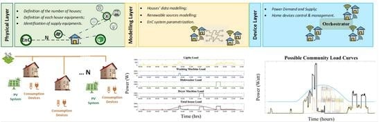
This EnC modelling framework can be represented by three distinct layers: physical, modelling, and device layer, as presented in Figure 5. The physical layer will provide a complete description of the community including the characterization of the houses inside the EnC (number of houses and tenants), the equipment (appliances) of each house, and the storage and supply equipment. The modelling layer will be responsible for the parametrization of all data collected from the first layer, as well as for the modelling of the renewable sources, storage devices, and household devices. Finally, the device layer manages the control of the system and the EnC flexibility. The demand, storage, and supply of each house, as well as the entire EnC, will be controlled through the device layer.
This EnC’s framework considers a 24-h active power diagram of demand and generation, and is given by Equations (1) and (2) respectively, where (d) denotes demand power and (g) denotes generated power.
N denotes the number of the considered EnC houses and t the time.
The community’s total demand (Td) and PV total generation (Tg) are given by Equations (3) and (4), respectively.
The supply and demand load of each house (including their flexibility), inside the community as well as for the entire EnC, will be handled in the device layer. Figure 6 presents the demand and generated power (Equations (1) and (2)), along with the load diagrams of the lights and three household-controlled devices (washing machine, dishwasher, and dryer machine). The washing machine load, for example, starts at 9h00 and its peak consumption is 2.5 kW, while dishwasher and dryer machine consumption reach 2 kW and their working cycle starts at 18h00 and 14h00, respectively. On Figure 6, the total house load represents the total consumption load as well as the load of available photovoltaic power.
2.1. Photovoltaic System
The PV system is modelled using Equation (5) considering the chosen PV panel information, the power inverter, ambient temperature (Tamb) and solar radiation data (G). Equation (5) provides the EnC house output power.
denotes the PV system peak power, the temperature coefficient of the maximum output power, the temperature of the PV panel cells and the reference cell temperature at standard test conditions (STC). The PV system’s peak power and the PV cells’ temperature are given by Equations (6) and (7), respectively.
In Equation (7), is the temperature of PV cell, is the ambient temperature, is the nominal operating cell temperature (NOCT), and is the ambient temperature and the solar radiation at NOCT, respectively.
2.2. Household Devices
Amongst the flexible household devices, this study considers event-based appliances that can be controllable and whose flexibility can be used without compromising the user’s comfort. The time profile of controllable appliances that can be chosen by the user presents different contours.
Controllable devices will be modelled as a generic finite state machine, as Figure 7 illustrates. The finite state machine has four different states (“Machine OFF”, “Machine Ready”, “Machine ON” and “Machine Complete”). The change between those states is done through a couple of signals defined by the user to characterize the appliance operation: “Ready_work” and “Time_ON”. “Appliance_Time” comes from the characteristics of each machine and the program chosen for its operation. For the sake of simplicity, the state machine in Figure 7 can be described with the support of the following example:
- The initial state is “machine OFF”, when the appliance is turned off,
- Once an appliance is ready to work the state changes to “Machine Ready” through the signal “ready_work”, and the appliance will be prepared to start its cycle when the time arrives,
- The signal “Time_ON” is triggered when the clock equals the starting time chosen by the user, changing the state to “Machine_ON”,
- The appliance will work during the time provided by the signal “Appliance_Time”, and the power that this appliance is consuming during its operation time will be the output of the state machine,
- When the appliance finishes its work, a signal, “complete”, is triggered that changes the appliance to “Machine_Complete” state,
- Finally, if the machine expects another cycle, the signal “cont_work” will be triggered and the state machine will stay in “Machine_Ready” state until the new signal to start working,
- Otherwise, the state “OFF” will be turned off the machine and the state will change to “machine_OFF”.
3. Proposed Methodology
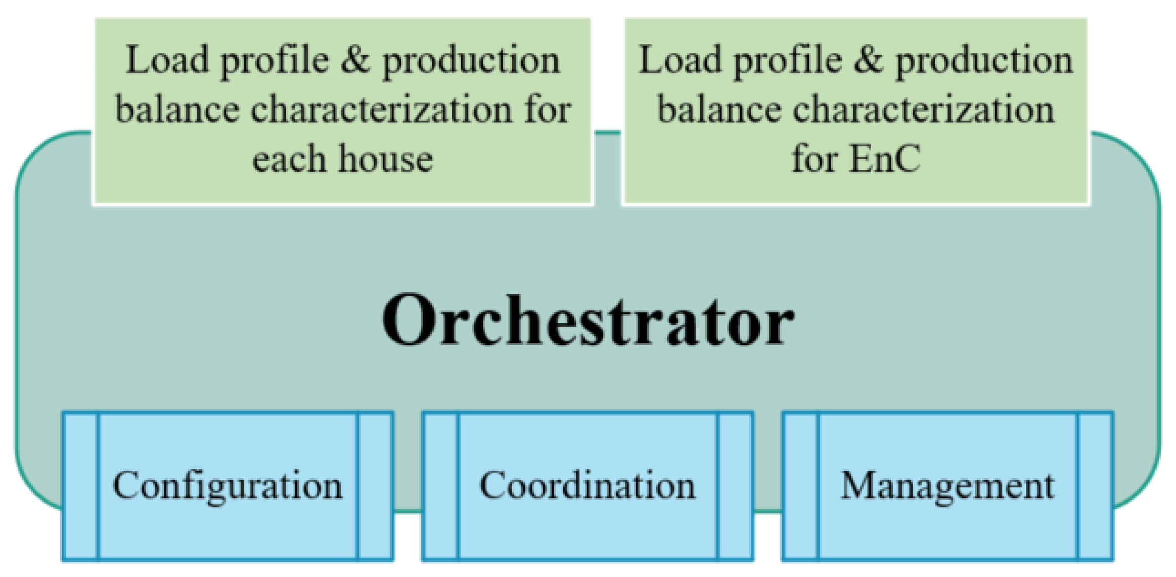
In this work, the proposed methodology considers as consumption appliances the event-based devices, such as dryer machine, washing machine, and dishwasher. The main component of the methodology is the “orchestrator”, which will aggregate and analyze data related to load and energy production profiles. Moreover, the orchestrator will also act as a decision support entity regarding the configuration, coordination, and management processes.
With the information about the working appliances introduced by the user, the load profile & production balance blocks compute the respective characterization of each house and for the EnC, respectively, as represented in Figure 8. This characterization will allow the orchestrator to configure, coordinate, and manage the EnC flexibility and needs.
Starting with the EnC configuration, considering the house’s characterization, the EnC characterization and the EnC connection to the main grid, the orchestrator analyzes the available power. The coordination starts with the system’s evaluation in order to understand if it is necessary to rearrange the demand. If necessary, each user’s flexibility will be used in three different ways (appliance’s earlier, mid, or later start), considering the restrictions presented below. In each proposed method, a permutation algorithm is used to calculate the number of possible combinations of appliances per house (Equation (8)), where a is the number of appliances. Afterwards, the combinations of household appliances are calculated (Equation (9)), where V is a vector with all load appliances and [a! a] is the size of the matrix with all combinations for each house.
Finally, the same algorithm is applied to study all possible combinations in order to have the best solution for community flexibility and the wellbeing maintenance of each user. Only the combinations that follow the condition presented in Equation (10), where t denotes time, will be considered as a possible demand rearrangement.
It is not always possible to keep all appliances working at the time requested by the user, or working at all. The appliances’ management inside the community is also done by the orchestrator (Figure 8). This management considers an optimization process that is presented below, considering different starting times when a fault is detected.
3.1. Restrictions
When a fault occurs or when there is insufficient power to feed the community’s grid, the system considers the following restrictions:
- If there are appliances already working, these ones will end their cycles whenever possible;
- Appliances that were supposed to work after the system activated will be moved to different starting times, and each one will work alone, i.e., in each house one appliance only starts after the previous has finished.
3.2. Optimization Process
The optimization process used in this study considers three different starting times for the appliances whenever a fault occurs and it is necessary to change the appliance’s load to other possible working hours different from the ones chosen by the users. The three different starting times, which use the same method and take into consideration the previously mentioned restrictions, are:
- Earlier Start: Each appliance’s starting time is moved to start as soon as possible after the management system detects the fault. In this way, each house’s amount of consumed power will be increased in order to have all appliances finish as soon as possible.
- Later Start: Each appliance’s starting time is moved to start as late as possible after the management system detects the fault, always considering the 24-h time interval. This approach will decrease the demand power in each house in order to have all appliances finish as late as possible.
- Mid Start: Each appliance’s starting time is moved towards a so-called midterm of appliance work, starting every n hours, inside the 24-h time interval and after the management system detects the fault. For example: if n is considered equal 4, and the fault was detected at 10h00, the mid start will work at 14h00, 18h00, and 22h00. This approach will force the loads to use the power of each house in the middle of the minimum, when the appliances work as late as possible, and maximum, when the appliances work as early as possible, available power.
From Figure 9, it is possible to visualize an example of a house load for a 24-h period where lights and the three different event-based appliances (washing machine, dish washer, and dryer machine) were considered. The original load diagram is presented in Figure 9a. The possible combinations of working load for the same house with an earlier, mid, and later start, respectively, are presented in Figure 9b–d.
In this illustrative example, the failure situation was detected at 10h00. This time is the fault time considered for all optimization process. It is possible to observe that the earlier start, Figure 9b, initiated at 10h00. The mid start will start 2 h after the fault time, at 12h00, and the later start began at 19h00, taking into consideration the 24 h interval, as represented in Figure 9c and d, respectively.
With flexibility curves of all houses belonging to the EnC, it is possible to combine them and find the ones that present the better combination of the appliances’ working times, maintaining the wellbeing of each user in their own dwellings.
In the next chapter, the scenarios, their results, and a detailed analysis will be presented.
4. Scenarios & Results Discussion
For this work, three different houses with consumption devices were considered, where one was equipped with a PV system and two were not, as depicted in Figure 10.
Taking into account the aforementioned system, to test the different possibilities for the community level, three distinct scenarios are considered:
- Scenario 1—in this scenario, the PV generation is the only available power inside the community.
- Scenario 2—in this scenario, the available power consists of PV generation and available power from the grid, with a general decrease of the grid’s available power.
- Scenario 3—in this scenario the available power consists of PV generation and available power from the grid working with power cut-offs, i.e., the power from the grid will decrease at a certain moment.
The algorithm behavior over a 24-h period (in order to study a complete day), considering the community’s necessities, is illustrated in Figure 11. First of all, the house and EnC load’s characterization and production balances are made, considering the available information. The algorithm takes into account: the type of fault scenario occurring, the information given by each house’s users, and the available power production. Taking that into consideration and, depending on the number of appliances and the needs of each house and of the entire community when a fault occurs, different possibilities of turning on the appliances at different moments of the day are presented.
For the simulations supporting this work, ambient temperature () and solar radiation () data was obtained from the photovoltaic geographical information system (PVGIS), with 15 min resolution and considering NOVA school of Science and Technology (38°39′36″ N/9°12′11″ W) as the location point. The values for the parametrization of the PV system are presented in Table 2.
Regarding household devices, the noncontrollable devices’ load is based on Richardson’s model [37]. As it is considered a noncontrollable device, the load used for each house is static. The controllable devices used for this work were exclusively of the event-based type, and their characteristics are presented in Table 3. The appliances and respective starting time for each house are also presented in Table 4.
For the sake of simplicity, a maximum of three appliances working per day was considered: washing machine, dryer machine, and dish machine. Using a dedicated application interface, as presented in Figure 12, the user can choose their corresponding starting time (hour:minute), and state if the house has a working PV panel.
Since batteries represent a big cost for communities at the present time, this study did not take them into account, considering only the power source coming from the PV panel and from the grid. Thus, scenario 1, which considers only power from PV production, as shown in Table 4, has some restrictions and the available power between 18h00 and 6h00 is equal to zero. In this time window, all appliances are disabled.
Considering each house’s characteristics, Figure 13 shows their respective demand profile, the total EnC demand, and the three different profiles of available power for each scenario to be tested. The “Community Demand & Generation” graph (Figure 13) presents the three scenarios, where it can be observed that a fault is detected at 10h00 and the community’s demand is higher than the available power. Under fault conditions, the algorithm will rearrange the appliances’ working time slot from 10h00 until 24h00, considering the amount of power available. The appliances already working before the fault occured are analyzed and, if necessary, they are put on pause and restarted when possible.
4.1. Scenario 1
The first scenario represents a particular case since the only power available for the community is provided by the PV system. This type of scenario will occur if a total cut off from the main grid happens and if the community does not have a storage system.
Considering the characteristics of the three houses presented in Table 4 and the solar curve shown in Figure 13 “Power Curve of House 2” graph (that has a peak power of 4 kW), an analysis will be done of the results of this scenario.
It is important to note that in time windows 00h to ~6h00 and ~18h00 to 24h00, the PV system does not produce, thus the community will not have power available during these time windows. Controllable appliances will work between 6h00 and 18h00.
As seen before, on the flowchart presented in Figure 11, when it is necessary to turn off some devices, the house with a PV system will have priority to maintain their appliances turned on. In this case, because of reduced available power, it was necessary to turn off the three appliances from house 1, maintaining only the noncontrollable devices, and two appliances from house 3, maintaining the dish washer (Table 5). The appliances that still work will have different starting times than the initial ones, since the optimization algorithm was applied to maintain the maximum number of appliances working.
In Figure 14, it is possible to see the community’s initial demand profile, the available power, and the two possible solutions that present a load profile smaller than the available power for the entire community. In this case, all possible solutions result in the characteristics presented in Table 5.
Despite the limitation regarding the available power to the community, and the necessity of turning off some appliances, two different solutions are presented in order not to turn off all the appliances of the community due to a total fault on the community’s grid.
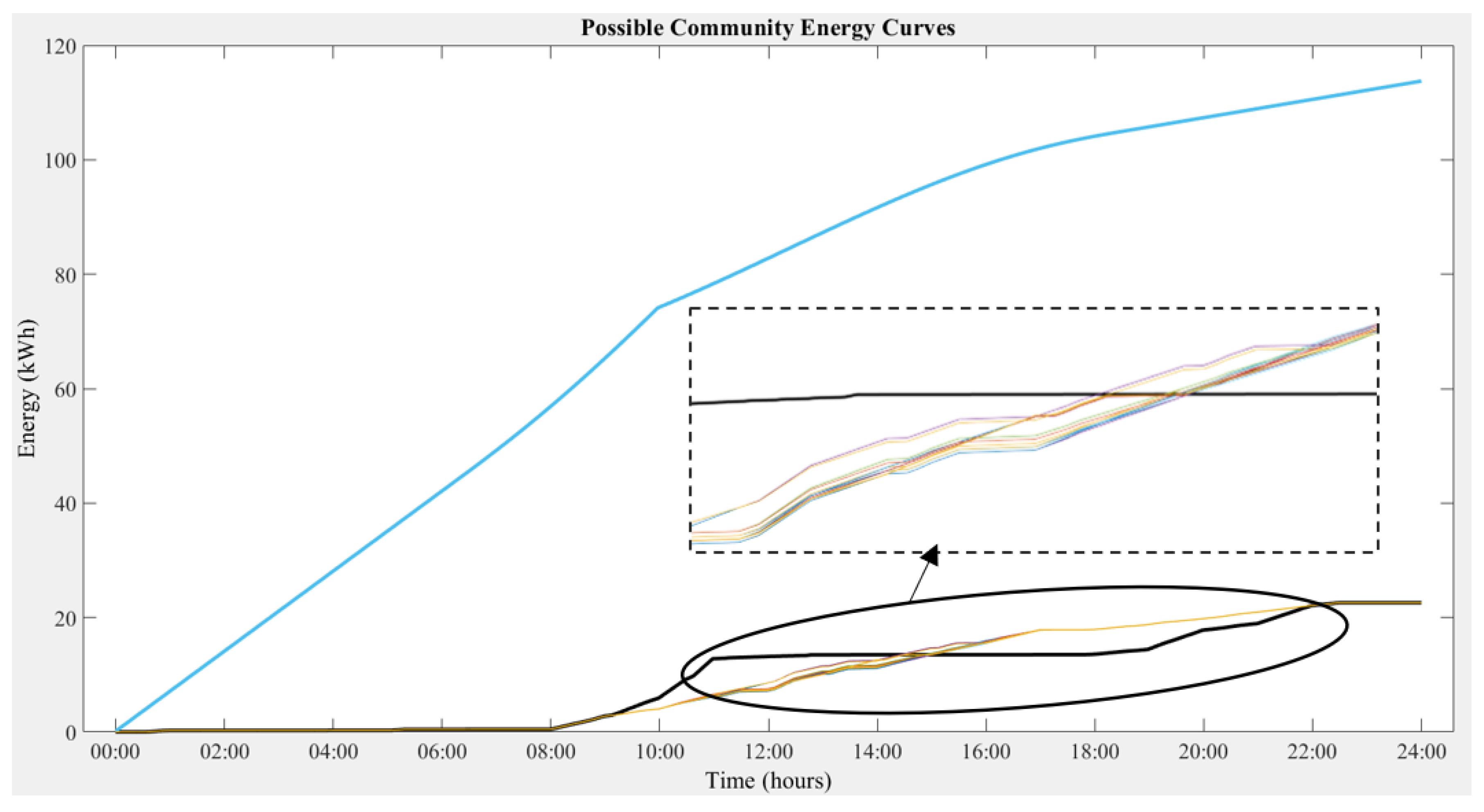
From Figure 14, the 24-h energy is easily computed using Equation (11), and is presented as accumulated energy during the day (Figure 15).
Considering the computed energy, and by analyzing Figure 15, the available energy corresponds to 21.4 kWh and the consumed energy corresponds to 9.39 kWh. This is the same amount as the initial consumed energy (without any fault), but appliances are turned on at different times of the day. This means that only 43.88% of the available energy is used.
In Figure 15, it is also possible to observe that the available energy curve is much higher than the consumed energy curves, and this is proven by the fact that only 43.88% of available energy is used. Despite that, the power available during the day varies, and is lower than the power consumption necessary to change the appliances’ working times. In this specific case, the need to turn off some devices is seen in this image, since the initial community energy is higher than the final possible solution.
4.2. Scenario 2
This scenario represents the usual working state inside the community, i.e., the available power inside the community comes from PV generation combined with power from the electrical grid. In this case, the decrease in power from the grid is general, and during the period of 24 h it represents 2 kW.
In contrast to scenario one, the community has power available during the entire 24 h window, but the demand is higher at 10h00. than the available power, and thus it is necessary to redistribute the appliances in order to maintain user wellbeing. In this case, it is possible to maintain all appliances being turned on, and 89 possible combinations can be considered. Some appliances, like the dryer and washer from house 2 and house 3, needed to be allocated earlier than the initial starting time since the available power at that time was insufficient to assure their operation. Figure 16 shows the curve of available power, the community’s demand, and the 89 possible reconfiguration combinations. It is important to mention that in this specific case, the appliance’s starting time will be concentrated at hours were the PV generation is higher. Moreover, the dryer washer in house 1 maintains its starting time since it starts at 8h00 and has a 1 h cycle, which allows it to work before the power decrease occurs.
Considering the energy computation from Figure 16 and the energy curves in Figure 17, it is possible to establish that the community has a total amount of 69.4 kWh of available energy and 22.59 kWh will be consumed, i.e., 32.53% of the available energy.
The behavior of different possible curves is shown in Figure 17, and compared with the initial community energy curve. In the first hours of the day (until approximately 14h00), the community’s flexibility is used to decrease its power consumption since the power available is lower than necessary. From 14h00 onwards, an increase in power consumption occurs until it matches the total amount of energy consumed during the day.
4.3. Scenario 3
In scenario 3, the community is connected to the main grid and receives 7 kW of power along with PV production from house 2. At 10h00, the power decreases from 7 kW to 1.6 kW, as shown in Figure 18. The power consumed is higher than the power available, and it is necessary to use the community’s flexibility in order to maintain all connections and users’ wellbeing. In this situation, every appliance from all three houses was maintained on. The power was decreased in the morning compared to the initial demand, and then increased in the afternoon in order to balance the load.
The available and consumed energy are 113.58 kWh and 22.59 kWh, respectively, as presented in Figure 19. Due to the initial power from the grid, the percentage of used energy, 19.89%, is lower compared with the other two scenarios. However, as in the second scenario, it was possible to maintain all user’s wellbeing. It is also possible to see that in the first few hours of the day, nothing is turned on when the changes occur. This happens because the proposed methodology considers real time actions and will only actuate from that time onwards.
4.4. Summary
An energy community with three houses was considered in this study. Noncontrollable and controllable devices in each house were considered as consumption sources. PV systems installed in the community’s houses and power coming from main grid were considered the power supply sources. The flexibility of each house inside the community was studied in order to decipher the community’s global flexibility and improve the controllable load management during a fault event. To assess the proposed methodology, three different scenarios were considered, with the differences between them being related to the available power in the community, as detailed in Table 6.
The first scenario only had available power from PV generation, implying that between certain times there was no available power. In the second and third scenarios, the available power comes from PV generation and the main grid. However, the second one had a generalized decrease and the available grid power was restricted to 2 kW during the 24 period. The third scenario started with 7kW of available power from the main grid that decreased to 1.6 kW, from 10h00 until midnight. The available energy inside EnC started at 21.4 kWh for scenario 1, increased to 69.4 kWh for scenario 2, and finished with 113.58 kWh for scenario 3, which is what was expected since the three scenarios present different levels of available power. The first one presents a lower level of availability due to the blackout between ~18 h and ~6 h, since the only available power source are PV panels.
From Table 6, one can see that the three scenarios started with the same set of characteristics for the EnC houses but finished with different results. In the first scenario, four devices were disconnected, the starting time for the other devices was changed, and houses 1 and 3 presented a lower energy consumption than the same houses in scenarios 2 and 3. Regarding scenario 1, it is also possible to see that, despite the need to disconnect devices, only ~44% of total energy available was used, meaning that, due to the lack of storage, 56% of available energy was wasted.
The same happened in scenarios 2 and 3. Although there was no need to disconnect any devices, only a small amount of energy was used.
5. Conclusions & Future Work
The aim of this paper was to explore the possibility of using the community’s energy flexibility to maintain the users’ wellbeing when a fault event occurs by considering an energy community with PV generation and houses with noncontrollable and controllable devices.
The simulation results showed the necessity of turning off some devices in order to maintain the community network when the available power is lower or experiences a small interval during a 24 h cycle. In this study, it was also possible to understand that houses’ energy flexibility can be further used to improve the community’s load in many ways, not only when a fault occurs and it is necessary to change the energy flow, but also for the purposes of creating better energy price markets, improving the resilience of the grid, or even connecting electrical vehicles to the community’s grid.
The values presented in Table 7 and the results of scenario 1, where only 44% of available energy was used, are a good example of this. Instead of turning off four devices and considering two blackout intervals, from 00 h to ~6 h and from ~18 h onwards, if the surplus energy had been stored, it could be used in those intervals, allowing the users to keep their appliances working.
The study performed in this research is a fundamental step towards achieving the following goals: (i) Definition of LV grid resilience and measurement metrics that will be used to assess the EnC resilience; (ii) Definition of KPIs to measure EnC’s energy flexibility; (iii) Definition of smart readiness indicators (SRI) to characterize the smartness of buildings/communities.
Moreover, when considering a real-world application of the energy community concept, some issues are still open and need to be further studied, namely:
- The integration of storage is an important issue that needs to be addressed in future work to store excess production so that it can be used when needed;
- The use of thermostatically controlled device flexibility;
- Penetration of electric vehicles in the EnC;
- Improved methods of studying and measuring a community’s resilience to better understand the relation between EnC flexibility and the improvement of EnC resilience.
Finally, regarding the replicability of this study, this methodology of flexibility can be applied to every type of energy community. It enables us to maintain the users’ wellbeing while using renewable production and sharing the available power between the users when needed.
Author Contributions
Conceptualization, A.M.; investigation, A.M.; supervision, P.P. and J.M.; writing—original draft, A.M.; writing—review, A.M., P.P. and J.M. All authors have worked on this manuscript together and all have read and approved the final manuscript.
Funding
This research was funded by “Fundação para a Ciência e Tecnologia” (FCT), grant number UIDB/00066/2020.
Institutional Review Board Statement
Not applicable.
Informed Consent Statement
Not applicable.
Data Availability Statement
Publicly available datasets were analyzed in this study. This data can be found here: https://ec.europa.eu/jrc/en/pvgis (accessed on 31 May 2021).
Acknowledgments
The authors acknowledge the infrastructure and support of the Department of Electrical and Computer—NOVA School of Science and Technology (FCT NOVA), and of the Centre of Technology and Systems, CTS—UNINOVA.
Conflicts of Interest
The authors declare no conflict of interest.
References
- Mar, A.; Pereira, P.; Martins, J.F. A survey on power grid faults and their origins: A contribution to improving power grid resilience. Energies 2019, 12, 4667. [Google Scholar] [CrossRef] [Green Version]
- Albert, R.; Albert, I.; Nakarado, G.L. Structural vulnerability of the North American power grid. Phys. Rev. E Stat. Nonlinear Soft Matter Phys. 2004, 69, 025103. [Google Scholar] [CrossRef] [Green Version]
- Crucitti, P.; Latora, V.; Marchiori, M. Model for cascading failures in complex networks. Phys. Rev. E Stat. Phys. Plasmas Fluids Relat. Interdiscip. Top. 2004, 69, 4. [Google Scholar] [CrossRef] [Green Version]
- Hines, P.; Balasubramaniam, K.; Sanchez, E.C. Cascading failures in power grids. IEEE Potentials 2009, 28, 24–30. [Google Scholar] [CrossRef]
- European Commission Shedding Light on Energy in the EU—A Guided Tour of Energy Statistics. Available online: https://ec.europa.eu/eurostat/cache/infographs/energy/ (accessed on 20 March 2021).
- Iddrisu, I.; Bhattacharyya, S.C. Sustainable Energy Development Index: A multi-dimensional indicator for measuring sustainable energy development. Renew. Sustain. Energy Rev. 2015, 50, 513–530. [Google Scholar] [CrossRef] [Green Version]
- Cohen, J.; Moeltner, K.; Reichl, A.; Schmidthaler, M. An empirical analysis of local opposition to new transmission lines across the EU-27. Energy J. 2016, 37, 59–82. [Google Scholar] [CrossRef]
- Azarova, V.; Cohen, J.; Friedl, C.; Reichl, J. Designing local renewable energy communities to increase social acceptance: Evidence from a choice experiment in Austria, Germany, Italy, and Switzerland. Energy Policy 2019, 132, 1176–1183. [Google Scholar] [CrossRef] [Green Version]
- Huang, Z.; Yu, H.; Peng, Z.; Feng, Y. Planning community energy system in the industry 4.0 era: Achievements, challenges and a potential solution. Renew. Sustain. Energy Rev. 2017, 78, 710–721. [Google Scholar] [CrossRef]
- IEC Technical Committee 1 (Terminology) IEC 60050—International Electrotechnical Vocabulary—Welcome. Available online: http://www.electropedia.org/ (accessed on 10 February 2020).
- Ceglia, F.; Esposito, P.; Maurizio, S. Smart Energy Community and Collective Awareness: A systematic Scientific and Normative Review. In Business Management Theories and Practices in a Dynamic Competitive Environment; EuroMed Press: Thessaloniki, Greece, 2019; pp. 139–149. ISBN 978-9963-711-81-9. [Google Scholar]
- Karunathilake, H.; Hewage, K.; Mérida, W.; Sadiq, R. Renewable energy selection for net-zero energy communities: Life cycle based decision making under uncertainty. Renew. Energy 2019, 130, 558–573. [Google Scholar] [CrossRef]
- Ziras, C.; Heinrich, C.; Pertl, M.; Bindner, H.W. Experimental flexibility identification of aggregated residential thermal loads using behind-the-meter data. Appl. Energy 2019, 242, 1407–1421. [Google Scholar] [CrossRef] [Green Version]
- Junker, R.G.; Azar, A.G.; Lopes, R.A.; Lindberg, K.B.; Reynders, G.; Relan, R.; Madsen, H. Characterizing the energy flexibility of buildings and districts. Appl. Energy 2018, 225, 175–182. [Google Scholar] [CrossRef]
- Lucas, A.; Jansen, L.; Andreadou, N.; Kotsakis, E.; Masera, M. Load Flexibility Forecast for DR Using Non-Intrusive Load Monitoring in the Residential Sector. Energies 2019, 12, 2725. [Google Scholar] [CrossRef] [Green Version]
- Bakhtavar, E.; Prabatha, T.; Karunathilake, H.; Sadiq, R.; Hewage, K. Assessment of renewable energy-based strategies for net-zero energy communities: A planning model using multi-objective goal programming. J. Clean. Prod. 2020, 272, 122886. [Google Scholar] [CrossRef]
- Ghiani, E.; Giordano, A.; Nieddu, A.; Rosetti, L.; Pilo, F. Planning of a smart local energy community: The case of berchidda municipality (Italy). Energies 2019, 12, 4629. [Google Scholar] [CrossRef] [Green Version]
- Burduhos, B.; Duta, A.; Moldovan, M. Nearly Zero Energy Communities, 1st ed.; Visa, I., Duta, A., Eds.; Springer International Publishing: Cham, Switzerland, 2018; ISBN 978-3-319-63214-8. [Google Scholar]
- Paci, S.; Bertoldi, D.; Shnapp, S.; Paci, D.; Bertoldi, P. Enabling Positive Energy Districts across Europe : Energy Efficiency Couples Renewable Energy; European Commission: Luxembourg, 2020. [Google Scholar]
- Pontes Luz, G.; Amaro E Silva, R. Modeling Energy Communities with Collective Photovoltaic Self-Consumption: Synergies between a Small City and a Winery in Portugal. Energies 2021, 14, 323. [Google Scholar] [CrossRef]
- Sarfarazi, S.; Deissenroth-Uhrig, M.; Bertsch, V. Aggregation of households in community energy systems: An analysis from actors⇔ and market perspectives. Energies 2020, 13, 5154. [Google Scholar] [CrossRef]
- EU Directive 2010/31/EU of the European Parliament and of the Council of 19 May 2010 on the Energy Performance of Buildings (Recast). 2010. Available online: https://eur-lex.europa.eu/legal-content/EN/TXT/?uri=celex%3A32010L0031 (accessed on 31 May 2021).
- Athienitis, A.; O’Brien, W. Modelling, Design, and Optimization of Net-Zero Energy Buildings; Wiley: Hoboken, NJ, USA, 2015; ISBN 9783433604625. [Google Scholar]
- Rehman, H.; Reda, F.; Paiho, S.; Hasan, A. Towards positive energy communities at high latitudes. Energy Convers. Manag. 2019, 196, 175–195. [Google Scholar] [CrossRef]
- Ala-Juusela, M.; Crosbie, T.; Hukkalainen, M. Defining and operationalising the concept of an energy positive neighbourhood. Energy Convers. Manag. 2016, 125, 133–140. [Google Scholar] [CrossRef] [Green Version]
- Walker, S.; Labeodan, T.; Maassen, W.; Zeiler, W. A review study of the current research on energy hub for energy positive neighborhoods. In Proceedings of the Energy Procedia; Elsevier: Amsterdam, The Netherlands, 2017; Volume 122, pp. 727–732. [Google Scholar]
- Bartholmes, J. Smart cities and communities. ITE J. Inst. Transp. Eng. 2017, 87, 36–38. [Google Scholar]
- Panteli, M.; Mancarella, P. The Grid: Stronger, Bigger, Smarter? IEEE Power Energy Mag. 2015, 13, 58–66. [Google Scholar] [CrossRef]
- Monti, A.; Pesch, D.; Ellis, K.A.; Mancarella, P. Energy Positive Neighborhoods and Smart Energy Districts; Elsevier: Amsterdam, The Netherlands, 2016; ISBN 978-0-12-809951-3. [Google Scholar]
- Reynders, G.; Amaral Lopes, R.; Marszal-Pomianowska, A.; Aelenei, D.; Martins, J.; Saelens, D. Energy flexible buildings: An evaluation of definitions and quantification methodologies applied to thermal storage. Energy Build. 2018, 166, 372–390. [Google Scholar] [CrossRef]
- Le Dréau, J.; Heiselberg, P. Energy flexibility of residential buildings using short term heat storage in the thermal mass. Energy 2016, 111, 991–1002. [Google Scholar] [CrossRef]
- Lopes, R.M.A. Extending Nearly Zero-Energy Buildings Load Matching Improvement to Community-Level, NOVA School of Science and Technology. 2017. Available online: https://run.unl.pt/handle/10362/29113 (accessed on 31 May 2021).
- Staats, M.R.; de Boer-Meulman, P.D.M.; van Sark, W.G.J.H.M. Experimental determination of demand side management potential of wet appliances in the Netherlands. Sustain. Energy Grids Netw. 2017, 9, 80–94. [Google Scholar] [CrossRef] [Green Version]
- Ur Rashid, M.M.; Granelli, F.; Hossain, M.A.; Alam, M.S.; Al-Ismail, F.S.; Karmaker, A.K.; Rahaman, M.M. Development of home energy management scheme for a smart grid community. Energies 2020, 13, 4288. [Google Scholar] [CrossRef]
- Stephant, M.; Abbes, D.; Hassam-Ouari, K.; Labrunie, A.; Robyns, B. Distributed optimization of energy profiles to improve photovoltaic self-consumption on a local energy community. Simul. Model. Pract. Theory 2021, 108. [Google Scholar] [CrossRef]
- Olivella-Rosell, P.; Lloret-Gallego, P.; Munné-Collado, Í.; Villafafila-Robles, R.; Sumper, A.; Ottessen, S.Ø.; Rajasekharan, J.; Bremdal, B.A. Local flexibility market design for aggregators providing multiple flexibility services at distribution network level. Energies 2018, 11, 822. [Google Scholar] [CrossRef] [Green Version]
- Richardson, I.; Thomson, M.; Infield, D. A high-resolution domestic building occupancy model for energy demand simulations. Energy Build. 2008, 40, 1560–1566. [Google Scholar] [CrossRef] [Green Version]
Figure 1.
Energy community scheme.

Figure 2.
Possible energy community faults.

Figure 3.
General Architecture of an energy community.

Figure 4.
Scheme of energy community under study.

Figure 5.
EnC modelling layers.

Figure 6.
Example appliances load.

Figure 7.
Appliances finite state machine.

Figure 8.
EnC decision support entity.

Figure 9.
Load profile of house 1: (a) Normal load; (b) Earlier start combinations; (c) Mid start combinations; (d) Later start combinations.
Figure 9.
Load profile of house 1: (a) Normal load; (b) Earlier start combinations; (c) Mid start combinations; (d) Later start combinations.

Figure 10.
EnC system studied.

Figure 11.
Community management system flowchart.

Figure 12.
House profile.

Figure 13.
House and community demand, house generation, and community power available for each scenario.
Figure 13.
House and community demand, house generation, and community power available for each scenario.

Figure 14.
Possible solutions for the community’s demand profile regarding Scenario 1.

Figure 15.
Community’s energy profile in Scenario 1.

Figure 16.
Possible solutions for the community’s demand profile regarding Scenario 2.

Figure 17.
The community’s energy profile in Scenario 2.

Figure 18.
Possible solutions for the community’s demand profile regarding Scenario 3.

Figure 19.
The community’s energy profile in scenario 3.


Table 1.
Household device type.
| Devices without storage | Without temporal displacement | Can be turned off | Lights, TVs, Computers |
| Cannot be turned off | Security systems | ||
| With temporal displacement (Event-based devices) | Washing machines, Dishwashers, Dryer machines | ||
| Storage Devices | Thermostatically controlled devices | Air conditioners, Heat pumps, Refrigerators, Electric water heaters | |
| Stochastic Devices | Electrical cars | ||
| Energy production devices | Cannot be controlled | Solar, Wind, Ocean | |
| Can be controlled | Biomass, H2 | ||
Table 2.
PV model & Inverter parameters used for the reference system with 4 kWp.
| PV System | Parameters | Value | Unit |
|---|---|---|---|
| PV Panel | A | 1.60 | m2 |
| PMPPT | 285 | Wp | |
| 46 | °C | ||
| 800 | Wm−2 | ||
| −0.003 | °C−1 | ||
| 20 | °C | ||
| 25 | °C | ||
| Pp | 4000 | W | |
| Sunny Tripower 4.0 Inverter | ηinv | 97.1 | % |
| PAC | 4000 | W |
Table 3.
Electrical appliance considered for this work.
| Appliance | Cycle Duration (min) | Mean Cycle Power (W) | Standby Power (W) | Controllable |
|---|---|---|---|---|
| Lights | Usage Dependent | Usage Dependent | 0 | No |
| Washing Machine (House 1; House 2; House 3) | 137 | 401 | 1 | Yes |
| Dryer Machine (House 1; House 2; House 3) | 59 | [1900; 2333; 2000] | 1 | Yes |
| Dishwasher (opt 1; opt2; opt3) | 59 | [2000; 1859; 2150] | 0 | Yes |
Table 4.
Houses’ initial characteristics.
| Houses | PV | Washing Machine | Dryer Wash | Dish Washer | Noncontrollable Devices |
|---|---|---|---|---|---|
| House 1 |  | 9h00 | 8h00 | 10h00 |  |
| House 2 | | 10h30min | 19h00 | 10h00 | |
| House 3 | | 10h30min | 21h00 | 9h30min | |
Table 5.
Houses’ final characteristics for Scenario 1.
| Houses | PV | Washing Machine | Dryer Wash | Dish Washer | Noncontrollable Devices (6 h–18 h) |
|---|---|---|---|---|---|
| House 1 | | | | | |
| House 2 | | 14 h | 13 h/12 h | 12 h/13 h | |
| House 3 | | | | 11 h | |
Table 6.
Scenario summary.
| Community Specs | Scenario 1 | Scenario 2 | Scenario 3 | ||||||
|---|---|---|---|---|---|---|---|---|---|
| Available power | PV generation only | PV generation & power from main grid with a general decrease 2 kW available | PV generation & power from main grid with cut-off at 10h00 From 7 kW to 1.6 kW | ||||||
| Energy Available (kWh) | 21.4 | 69.4 | 113.58 | ||||||
| Possible Curves | 2 | 89 | 24 | ||||||
| Turned off Devices | 4/9 (44%) | 0/9 (0%) | 0/9 (0%) | ||||||
| Total energy used (%) | 43.88 | 32.53 | 19.89 | ||||||
| Houses’ initial characteristics (same for 3 scenarios) | House 1 | House 2 | House 3 | ||||||
| PV | | | | ||||||
| Washing Machine | 09h00 | 08h00 | 10h00 | ||||||
| Dryer Machine | 10h30min | 19h00 | 10h00 | ||||||
| Dish Washer | 10h30min | 21h00 | 09h30min | ||||||
| Noncontrollable devices | | | | ||||||
| Houses’ final characteristics | House 1 | House 2 | House 3 | The same as initial | The same as initial | ||||
| PV | | | | ||||||
| Washing Machine | | 14h00 | | ||||||
| Dryer Machine | | 13h00/12h00 | | ||||||
| Dish Washer | | 12h/13h00 | 11h00 | ||||||
| Noncontrollable devices | | | | ||||||
| Energy consumption (kWh) | House1 | House2 | House3 | House1 | House2 | House3 | House1 | House2 | House3 |
| - | 7.64 | 4.52 | 7.35 | 7.64 | 7.59 | 7.35 | 7.64 | 7.59 | |
Table 7.
Scenario brief comparison.
| Community | Scenario 1 | Scenario 2 | Scenario 3 |
|---|---|---|---|
| Energy Available (kWh) | 21.4 | 69.4 | 113.58 |
| Possible Curves | 2 | 89 | 24 |
| Turned off Devices | 4/9 (44%) | 0/9 (0%) | 0/9 (0%) |
| Energy used (%) | 43.88 | 32.53 | 19.89 |
Publisher’s Note: MDPI stays neutral with regard to jurisdictional claims in published maps and institutional affiliations. |
© 2021 by the authors. Licensee MDPI, Basel, Switzerland. This article is an open access article distributed under the terms and conditions of the Creative Commons Attribution (CC BY) license (https://creativecommons.org/licenses/by/4.0/).
Share and Cite
MDPI and ACS Style
Mar, A.; Pereira, P.; Martins, J. Energy Community Flexibility Solutions to Improve Users’ Wellbeing. Energies 2021, 14, 3403. https://0-doi-org.brum.beds.ac.uk/10.3390/en14123403
AMA Style
Mar A, Pereira P, Martins J. Energy Community Flexibility Solutions to Improve Users’ Wellbeing. Energies. 2021; 14(12):3403. https://0-doi-org.brum.beds.ac.uk/10.3390/en14123403
Chicago/Turabian StyleMar, Adriana, Pedro Pereira, and João Martins. 2021. "Energy Community Flexibility Solutions to Improve Users’ Wellbeing" Energies 14, no. 12: 3403. https://0-doi-org.brum.beds.ac.uk/10.3390/en14123403
Note that from the first issue of 2016, this journal uses article numbers instead of page numbers. See further details here.