Optimization for Data-Driven Preventive Control Using Model Interpretation and Augmented Dataset

Abstract

Transient stability preventive control (TSPC) ensures that power systems have a sufficient stability margin by adjusting power flow before faults occur. The generation of TSPC measures requires accuracy and efficiency. In this paper, a novel model interpretation-based multi-fault coordinated data-driven preventive control optimization strategy is proposed. First, an augmented dataset covering the fault information is constructed, enabling the transient stability assessment (TSA) model to discriminate the system stability under different fault scenarios. Then, the adaptive synthetic sampling (ADASYN) method is implemented to deal with the imbalanced instances of power systems. Next, an instance-based machine model interpretation tool, Shapley additive explanations (SHAP), is embedded to explain the TSA model’s predictions and to find out the most effective control objects, thus narrowing the number of control objects. Finally, differential evolution is deployed to optimize the generation of TSPC measures, taking into account the security and economy of TSPC. The proposed method’s efficiency and robustness are verified on the New England 39-bus system and the IEEE 54-machine 118-bus system.

1. Introduction

1.1. Background

The power system is a strategic system for national economic development. Its safety and stability are of great significance to ensuring the electrical power supply. In the course of social development, there inevitably are situations where the network or the operation of power systems is not compatible with power supply demand, bringing the operating point close to the stability limit and bringing a significant challenge to the dispatch and control of power systems. The increasing uncertainty of the intermittent renewable generation and load demand, and transmission line unavailability threaten the security of power systems [1,2,3]. Transient instability is often the main reason for large-scale accidents in power systems. Practical transient stability assessment (TSA) and transient stability preventive control (TSPC) of power systems are the keys to preventing accidents [4,5]. TSPC is usually performed as power generation rescheduling. The safe operation of power systems is of primary concern. However, in the context of the electricity market and sustainable development, the economic operation of power systems cannot be ignored either. Therefore, a trade-off between safety, economy, and efficiency needs to be considered in preventive control.

1.2. Research Review

In most studies, the generation of TSPC strategies is defined as a global mathematical optimization problem, usually solved by dynamic security-constrained optimal power flow [6]. The dynamic security constraints include small signal stability constraints [7], voltage stability constraints [8], and transient stability constraints [9,10,11,12].

In this paper, we focus on the transient stability constrained optimal power flow (TSCOPF). A variety of methods of TSCOPF have been proposed in the past few years [9,10,11,12,13,14,15,16,17,18,19,20,21,22,23,24,25,26,27,28,29,30,31,32,33,34]. In general, TSCOPF-based TSPC is generally divided into two steps:

(1) Define transient stability constraints according to the state variables of power systems and the transient stability index (TSI), ensuring that the generators in the power systems can maintain synchronization after expected failures. Some mainstream TSIs are classified as follows: (a) transient energy [4], determined by the kinetic and potential energy of a post-fault power system; (b) stability margin [5] or critical clearing time [9] based on extended equal area criterion; and (c) the maximum rotor angle difference of the system in the transient process [10,11,12].

(2) Incorporate the transient stability constraints into the traditional optimal power flow solution model, and solve the optimal power flow. Abhyankar, S. and Geng, G. et al. summarized the taxonomy of a series of state-of-the-art for the solution of TSCOPF [13,14], including the following:

• Intelligent heuristic algorithms [12,15,16,17,18,19,20,21]. A variety of methods of intelligent heuristic algorithms were introduced to solve the TSCOPF, including swarm intelligence algorithms (particle swarm optimization [12] and improved micro-particle swarm optimization [15]) and evolutionary algorithms (genetic algorithm [16,17,18], non-dominated sorting genetic algorithm-II [19], and differential evolution (DE) [20,21]).
• Deterministic programming techniques [22,23,24,25,26,27,28]. Ledesma, P. et al. proposed a multi-contingency TSCOPF model that retained the high-level dynamics of all generators and solved the model using a non-heuristic interior point method (IPM) [22]. Pizano-Martinez A. et al. introduced the Single Machine Equivalent method to diminish the size of the optimization problem, overcoming the main drawback of global TSCOPF techniques (its huge dimension) [23,24]. Jiang, Q. et al. proposed improved numerical discretization and primal-dual IPM, significantly improving the computation efficiency of TSCOPF [25,26]. Francisco, A. et al. integrated a flywheel model in a multi-contingency TSCOPF and solved TSCOPF using IPM [27]. Arredondo, F. et al. solved TSCOPF with primal-dual IPM in the condition of a high share of renewable energy [28].
• An hybrid method combining classical deterministic programming technique and evolutionary algorithm [29].

Machine learning was introduced to construct transient stability constraints to meet the rapid generation of TSPC strategies [5,31,32,33,34]. With the characteristics of offline training and online real-time prediction, machine learning models can quickly assess the stability of power systems and judge whether it is within the transient stability constraints, realizing the rapid generation of TSPC strategies. However, there are still two problems to be solved.

The first problem is that there are too many expected contingency scenarios, and thus, it is unrealistic to construct TSA models for each given contingency scenario. Therefore, it is necessary to build a synthetic TSA model suitable for all expected faults.

The second problem is that many generators exist in practical power systems, where it is not economical to schedule the generators globally. Therefore, the scope of dispatch control needs to be narrowed to meet the requirements of precision and economy.

1.3. Contributions

The contributions of this paper consist of developing an enhanced data-driven preventive control strategy for a more effective and precise search for global optima of TSCOPF using model interpretation and augmented dataset method.

• In response to the first problem, an augmented dataset for training the TSA model is constructed by adding fault information to the traditional TSA dataset, thus improving the accuracy and the generalization ability of the TSA model. The novel TSA model trained by the proposed dataset can adapt to the multi-contingency condition without paying much more computation complexity. In addition, adaptive synthetic sampling (ADASYN) is adopted to generate a balanced dataset by synthesizing a group of minority class instances.
• As for the second problem, the most effective control objects are screened to narrow the adjustment objects in TSCOPF using an instance-based interpretation method, Shapley additive explanations (SHAP). Unlike some model-based global analysis approaches, SHAP can locate the most influential control objects for the individual current operation point, thus accomplishing more effective preventive control. Furthermore, DE is implemented to solve TSCOPF to minimize the operation and control cost, considering the transient stability constraints and economic factors.

The rest of this paper is structured as follows. Section 2 gives a detailed introduction of the proposed TSPC methodology, including a general framework and some specific techniques. Section 3 presents the numerical results of the proposed strategy in the two benchmark systems, the New England 39-bus system and the IEEE 54-machine 118-bus system, verifying the feasibility of the proposed method. Finally, the main conclusions and prospects of this paper are summarized and highlighted in Section 4.

2. Proposed Methodology

2.1. General Framework

The general framework of the proposed method is divided into two stages, an offline stage and an online stage, as illustrated in Figure 1.

TSA machine learning models are trained by a time-domain simulation (TDS) dataset covering fault information in the offline stage. ADASYN is deployed to deal with the imbalance in the TDS dataset. In addition, the dataset is preprocessed by outlier detection and normalization. Then, the TSA models, including a predictor and a classifier, are generated. The predictor outputs the predicted stability probability, and the classifier implements instance classification according to the predicted stability probability and a predetermined classification threshold.

In the online stage, the data of power systems are obtained in real-time. The trained classifier is used to monitor the N − 1 stability of the current operating status of power systems. Once the instability is identified, the mechanism of SHAP is triggered. The generators or loads that have a more significant influence on the stability are regarded as candidate control objects. Furthermore, TSCOPF is solved to calculate the control amount, where the predictor provides the transient stability constraint. Next, N − 1 TSA is performed on the preliminary generated TSPC measures by TDS or machine learning. If the result of the stability check is stability, TSPC is activated. Otherwise, the control objects and their amount are readjusted.

2.2. Dataset Covering Fault Information

Since TSPC is implemented before the fault, the data of the TSA models applied to TSPC must also be the pre-fault steady-state variables of power systems. In most of the literature, a set of TSA models are constructed based on specific expected faults. With the increase in faults, the cost of model training, storage, and maintenance increases, which is not suitable for large-scale power systems. In addition, since there is a certain similarity or correlation in fault characteristics and in the post-fault state of power systems for different faults, the TSA models between different faults can be aggregated. Based on the original TSA model dataset, the information of the expected line faults is included, as shown in

Table 1. Augmented TSA dataset covering fault information.

Type	Description
Fault	Fault line ($Lin{e}_f$)
	Fault location
	Rated Voltage
	Fault duration
	Transition resistance
Generator	Active power output ($P_{Gi}$)
	Reactive power output ($Q_{Gi}$)
	Voltage amplitude of bus ($V{m}_{Gi}$)
	Voltage phase angle of bus ($V{a}_{Gi}$)
AC line	Active transmission power ($P_{ACi}$ or $P_{Linei-j}$)
	Reactive transmission power ($Q_{ACi}$ or $Q_{Linei-j}$)
Load	Active power ($P_{Li}$)
	Reactive power ($Q_{Li}$)
	Voltage amplitude of bus ($V{m}_{Li}$)
	Voltage phase angle of bus ($V{a}_{Li}$)

, aiming to aggregate the stability laws of different faults. The datasets for other types of failures can be constructed similarly.

2.3. Adaptive Synthetic Sampling in TSA

TSA based on machine learning is essentially a classification problem, which requires sufficient and relatively balanced data to train a TSA model. If the data are imbalanced, the trained model is unreliable. For example, in 100 instances, category A accounts for 95%while category B accounts for only 5%. Suppose that the trained model discriminates all instances as A. Then, the accuracy is 95%, which definitely cannot accurately reflect the model’s performance. In power systems, the amount of the actual instability data is small, and at the same time, the instances of TDS may also face the problem of an imbalance. Therefore, in this paper, ADASYN is introduced in the framework of TSA.

The core idea of ADASYN is to generate different numbers of new instances of minority classes according to their learning levels. The level of learning for minority instances is expressed by the number of majority classes around minority samples. ADASYN adaptively transfers the classification boundary to difficult-to-learn instances and reduces the bias introduced by the initial imbalance data distribution. The specific ADASYN algorithm refers to Reference [35].

The performance indices, including accuracy, precision, recall, F1_score, and G_mean, are formulated as (1)–(5), where TP represents the number of instances truly predicted as positive, TN represents the number of instances truly predicted as negative, FP represents the number of instances falsely predicted as positive, and FN represents the number of instances falsely predicted as negative.

$$Accuracy=\frac{TP+TN}{TP+TN+FP+FN}$$

(1)

$$Precision=\frac{TP}{TP+FP}$$

(2)

$$Recall=\frac{TP}{TP+FN}$$

(3)

$$F1\_score=\frac{2·Precision·Recall}{Precision+Recall}$$

(4)

$$G\_mean=\sqrt{\frac{TP}{TP+FN}·\frac{TN}{TN+FP}}$$

(5)

Precision is intuitively the ability of the classifier to not label a sample that is negative as positive. Recall is intuitively the ability of the classifier to find all of the positive samples. The F1_score can be interpreted as a weighted average of the precision and recall, where an F1_score reaches its best value at 1.0 and its worst at 0. The relative contributions of precision and recall to the F1_score are equal. G_mean characterizes the average accuracy of minority and majority classes without sacrificing any category.

2.4. Determination of Control Objects Based on Shapley Values

In general, deep learning models are a kind of black box. Although the prediction results of deep learning models can be easily obtained, the internal prediction logic of for specific instances is hidden from their users. Due to the requirements of safety and reliability of power systems, the unexplainable TSA models make it difficult for operators and dispatchers to trust and apply them thoroughly. Model interpretation provides a way to open the black-box models, making models more informative and easier to understand.

Strumbelj, E. et al. [36] proposed an instance-based model interpretation method, SHAP, introducing Shapley values to interpret machine learning models in the image and text recognition domains. Shapley values represent a kind of feature importance, computed based on a game-theoretic solution with the idea of permutation. The specific definition of Shapley values is as follows:

The importance of the ith feature for a specific sample x is defined as ${\phi }_i\left(x\right)$.

$${\phi }_i\left(x\right)=\frac{1}{n!}\sum _{\mathcal{O}\in \pi \left(n\right)}(\Delta (P{r}^i\left(\mathcal{O}\right)\cup \left\{i\right\})\left(x\right)-\Delta \left(P{r}^i\left(\mathcal{O}\right)\right)\left(x\right))$$

(6)

$$\Delta \left(Q\right)\left(x\right)=\sum _{y\in \mathcal{A}}p\left(y\right)(f\left(\tau (x,y,Q)\right)-f\left(y\right))$$

(7)

$\mathcal{A}\in {\mathcal{A}}_1\times {\mathcal{A}}_2\times ...\times {\mathcal{A}}_n$ is an n-dimension feature space. $Q\subseteq S=\{{\mathcal{A}}_1,...,{\mathcal{A}}_n\}$ is a certain subset of features in a given sample $x\in \mathcal{A}$, and $\Delta \left(Q\right)\left(x\right)$ represents its influence. Function $f:\mathcal{A}\to \mathcal{R}$ is an regression model. For a classification model, f could be the probabilistic prediction of classification. p is the probability of a given sample $y\in \mathcal{A}$. $\tau (x,y,W)=(z_1,z_2,...,z_n)$, where $z_i=x_i$ iff $i\in W$ and $z_i=y_i$ otherwise. $\pi \left(n\right)$ is the set of all permutations of n elements, and $P{r}^i\left(\mathcal{O}\right)$ is the set of all features that precede the ith feature in permutation $\mathcal{O}\in \pi \left(n\right)$.

The approximating algorithm for the Shapley value is intuitively shown in Algorithm 1, where the permutation $\mathcal{O}$ and the assistant sample y are selected at random. K is the number of background data used to calculate the Shapley value.

The background dataset is used for integrating the features. For small-scale problems, this background dataset can be the whole training set, but for larger-scale problems, consider using a single reference value or using the k-means function to summarize the dataset, which will reduce the time cost of interpretation. If background data are used to calculate the Shapley values without being summarized, the operation matrix would be too large, resulting in insufficient allocated memory. The classical k-means algorithm is as follows.

• Step 1: Select K samples from the dataset x as the initial clustering center c randomly.
• Step 2: For each sample $x_i$, calculate its distances to K clustering centers and classify the sample to the class C corresponding to the nearest clustering center.
• Step 3: Recompute the clustering center c for each class $C_k$, $c_k\leftarrow \frac{1}{|c_k|}{\sum }_{x\in C_k}x$.
• Step 4: Repeat steps 2 and 3 until the termination conditions are satisfied, such as the convergence of clustering centers and the maximum number of iterations.

Algorithm 1 Calculating Shapley value ${\phi }_i\left(x\right)$, the importance of the ith feature for sample x and model f. Take K samples.

${\phi }_i\left(x\right)\leftarrow 0$ for$k\leftarrow 1$ to K do   select permutation $\mathcal{O}\in \pi \left(n\right)$ and sample $y\in \mathcal{A}$ randomly   $x_1:\{{\mathcal{A}}_1,...,{\mathcal{A}}_{i}fromxin\mathcal{O}\}\cup \{{\mathcal{A}}_{i+1},...,{\mathcal{A}}_{n}fromyin\mathcal{O}\}$   $x_2:\{{\mathcal{A}}_1,...,{\mathcal{A}}_{i-1}fromxin\mathcal{O}\}\cup \{{\mathcal{A}}_i,...,{\mathcal{A}}_{n}fromyin\mathcal{O}\}$   ${\phi }_i\left(x\right)\leftarrow {\phi }_i\left(x\right)+f\left(x_1\right)-f\left(x_2\right)$ end for ${\phi }_i\left(x\right)\leftarrow \frac{{\phi }_i\left(x\right)}{K}$

In order to improve the convergence speed of k-means in the iterative process and to reduce the time elapsed, k-means++ algorithm [37] is introduced to initialize the cluster centers. The k-means++ algorithm is as follows.

• Step 1: Select one sample of the dataset x as the initial clustering center $c_1$ randomly.
• Step 2: Calculate the minimum distance of each sample $x_i$ to the current clustering center, represented by $D\left(x_i\right)$.
• Step 3: For each sample, calculate the probability of being selected as the next clustering center, $\frac{D{\left(x_i\right)}^2}{{\sum }_{x_i\in x}D{\left(x_i\right)}^2}$.
• Step 4: Determinate the next clustering center with the roulette wheel method.
• Step 5: Repeat steps 2, 3, and 4 until K clustering centers are identified.
• Step 6: The rest procedures are the same as steps 2, 3, and 4 in the classical k-means.

Moreover, the Shapley values of features have a welcome nature that they are implicitly normalized, satisfying (3), where $f_{base}$ is the average prediction of all background samples. Thus, the interpretation results can explain how the machine learning model’s output is pushed from the base value to the final prediction by each feature’s influence.

$$f\left(x\right)=f_{base}+\sum _i^n{\phi }_i\left(x\right)$$

(8)

In power systems, especially in TSA and TSPC, unstable instances are often of great concern. In the TSPC stage, dispatchers scan and assess N − 1 contingency in the entire power system, looking for volatile failures to improve the stability margin of the power system by rescheduling the power generation. In this paper, SHAP is used to obtain each feature’s Shapley values and to explain the unstable instances. Then, the features are ranked according to Shapley values, representing the feature importance for the instances. The top-k important features are taken. Since the objects of TSPC must be controllable, the importance of controllable features needs to be identified and ranked. Define the importance of the ith controllable feature ($I_{ctrl}\left(i\right)$) as the weighted sum of the absolute values of the Spearman correlation coefficients ($cc$) of the top-k important features and the controllable features, where the weights are the absolute values of Shapley values ($\phi$) of the top-k important features.

$$I_{ctrl}\left(i\right)=\sum _j^k|c{c}_{ij}|·|{\phi }_j|$$

(9)

Define m as the number of the control objects of TSPC. The alternative identification strategies of m are as follows.

(a)

Manual identification according to expert experience.

(b)

Automatic identification with the importance margin ${ϵ}_{imp}$ of controllable features, as (10)–(12).

(c)

Automatic identification according to simulations for TSIs of multiple TSPCs.

$$\begin{array}{cc}\hfill & m=min\left(k\right)\hfill \end{array}$$

(10)

$$\begin{array}{cc}\hfill s.t.& \frac{{\sum }_i^k{\widehat{I}}_{ctrl}\left(i\right)}{{\sum }_i^n{\widehat{I}}_{ctrl}\left(i\right)}>{ϵ}_{imp}\hfill \end{array}$$

(11)

$$\begin{array}{cc}\hfill & {\widehat{I}}_{ctrl}\left(i\right)=\frac{I_{ctrl}\left(i\right)}{{\sum }_i^n{I}_{ctrl}\left(i\right)}\hfill \end{array}$$

(12)

According to a ranking of the importance of controllable features, the first-m controllable features with a strong correlation with system instability are selected as the candidate control objects. As a result, the scope of control objects is narrowed, laying the foundation for an economical TSPC.

2.5. TSCOPF Based on Differential Evolution

A TSCOPF problem can be formulated as the minimum of the sum of control cost and operation cost with three types of constraint conditions, (13)–(20). The constraints of TSCOPF include (1) power flow constraints, (2) steady-state constraints (upper and lower limits constraints of generator active, reactive power output, and bus voltage magnitude, and thermal limits of lines, respectively), and (3) transient stability constraints.

$$\begin{array}{cc}\hfill Min.& \sum _i^{n_G}|\Delta P_{Gi}|C_{Gi}+\sum _i^{n_G}(a_i+b_i{P}_{Gi}+c_i{\left(P_{Gi}\right)}^2)\hfill \end{array}$$

(13)

$$\begin{array}{cc}\hfill s.t.& P_G-P_L-P(V,\theta )=0\hfill \end{array}$$

(14)

$$\begin{array}{cc}\hfill & Q_G-Q_L-Q(V,\theta )=0\hfill \end{array}$$

(15)

$$\begin{array}{cc}\hfill & P_{Gmin}\le P_G\le P_{Gmax}\hfill \end{array}$$

(16)

$$\begin{array}{cc}\hfill & Q_{Gmin}\le Q_G\le Q_{Gmax}\hfill \end{array}$$

(17)

$$\begin{array}{cc}\hfill & V_{min}\le V\le V_{max}\hfill \end{array}$$

(18)

$$\begin{array}{cc}\hfill & S(V,\theta )\le S_{max}\hfill \end{array}$$

(19)

$$\begin{array}{cc}\hfill & f_{thr}-f(·)\le 0\hfill \end{array}$$

(20)

In the above formula, (13) is the cost function; $P_{Gi}$ is the active power of generator i; $\Delta P_{Gi}$ is the adjustment of the active power of generator i; $C_{Gi}$ is the unit adjustment cost of the active power of generator i; $n_G$ is the number of generators; $a_i$, $b_i$, and $c_i$ are the coefficients of the operation cost function of generator i; (14) and (15) are the active and reactive power balance constraints; $P_G$ and $Q_G$ are the vectors of generator active and reactive power output, respectively; $P_L$ and $Q_L$ are the vectors of active and reactive load, respectively; V and $\theta$ are the vectors of bus voltage magnitudes and angles, respectively; (16)–(19) are the steady-state constraints; $P_{Gmin}$, $P_{Gmax}$, $Q_{Gmin}$, $Q_{Gmax}$, $V_{min}$, and $V_{max}$ are the vectors of the lower and upper limits of the generator’s active and reactive power outputs, and the bus voltage magnitudes, respectively; $S(V,\theta )$ is the vector of apparent power flowing across the transmission lines, and $S_{max}$ is the vector of thermal limits of those lines; (20) is the transient stability constraints; $f(·)$ is the function of the security boundary given by dynamic variables; and $f_{thr}$ is a suitable threshold value.

The control cost of the active power of generators can further be divided into an upward adjustment cost and a downward adjustment cost. In order to simplify the case analysis, the control cost is not considered in the case.

Transient stability constraints are constructed by TSA machine learning models. The stability probability of TSA is taken as the security boundary, $f(·)$. For a binary classification problem, the threshold, $f_{thr}$ is usually set to 0.5. However, for power system stability control, the threshold can be increased appropriately.

In addition, TSI is based on the maximum rotor angle difference ($\Delta {\delta }_{max}$) of the power system. When TSI is less than 0, the system is unstable; when TSI is greater than 0, the system is stable.

$$\mathrm{TSI}=\frac{{360}^{\circ }-|\Delta {\delta }_{max}|}{{360}^{\circ }+|\Delta {\delta }_{max}|}$$

(21)

The differential evolution algorithm is essentially one of the population-based heuristic search algorithms that are suitable for continuous space and can achieve multi-objective optimization. Therefore, in this paper, TSCOPF is solved by using DE (DE-TSCOPF). DE algorithm originates from the idea of genetic algorithm (GA), including mutation, crossover, and selection. Different from GA, in the genetic process of DE, the mutation vector is generated from the parental differential vector and crosses the parental individual vector to generate a new individual vector. Then, the dominant individual is selected among the newborn individual and its parental individuals. The specific DE algorithm refers to Reference [38].

Our optimization strategy of TSPC is universal. Besides DE, most other approaches of TSCOPF can be suitably incorporated into our strategy, whether it is a heuristic algorithm or a mathematical approach.

3. Results and Discussion

In order to demonstrate the applicability of the proposed method, two benchmark systems are tested, including the New England 10-machine 39-bus system and the IEEE 54-machine 118-bus system. The simulations and tests are implemented on a PC with an Intel Core i5-2400 CPU and 4.00 GB of RAM, and the real-time measurement is replaced by the simulated data. The power flow calculation results are obtained using the MATPOWER 6.0 package, and TDS is performed in PSAT.

3.1. New England 10-Machine 39-Bus System

3.1.1. Dataset Generation

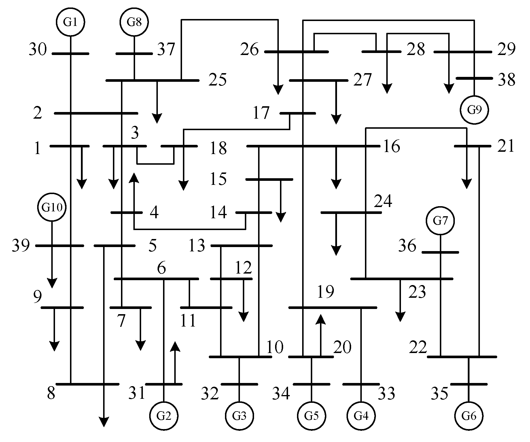
The single line diagram of the New England 10-machine 39-bus system is illustrated in Figure 2. The expected faults are determined based on the N − 1 contingency criterion. The operation data are generated with the Monte Carlo method for each fault, and TDS is performed. All faults are set as the most severe three-phase metallic short-circuit fault with a transient resistance of 0.001 $\mathsf{\Omega }$. The duration is randomly selected within 0.1–0.3 s, and the fault location is randomly selected within 0–100%. The data are labeled by TSI after TDS. Finally, an augmented dataset covering fault information is obtained.

In the simulations, all data about the fault of line AC 22 (BUS 16-BUS 19) in the augmented dataset are labeled as unstable, indicating that neither the TDS method nor the machine learning method can generate TSPC measures against the line fault. In this case, the fault of line AC 22 is handled in the emergency control stage. Therefore, it is assumed in this paper that the fault on line AC 22 is ignored during the preventive control stage.

After eliminating the outliers, a total of 2947 stable instances and 221 unstable instances are generated, indicating that the dataset is imbalanced. After implementing ADASYN, a balanced dataset is finally obtained, containing 2947 stable instances and 2518 unstable instances.

3.1.2. Transient Stability Assessment

Multi-layer perceptron (MLP) is selected as the prototype of TSA models. The structure of MLP is [500-100-50-10]. In total, four TSA models are tested, including the original TSA model, the TSA model with a dataset covering fault information, the TSA model with a balanced dataset augmented by ADASYN, and the proposed TSA model constructed using both dataset-augmenting techniques listed above. The performance of the TSA models is shown in

Table 2. Performance of transient stability assessment models in the New England 10-machine 39-bus system.

Type	Accuracy (%)	Precision (%)	Recall (%)	F1_Score (%)	G_Mean (%)
Original	95.6	97.0	98.3	97.7	75.0
Fault information	96.1	96.7	99.2	97.9	72.1
ADASYN	98.8	99.0	98.8	98.9	98.8
Fault information + ADASYN	99.2	99.2	99.3	99.2	99.2

.

The accuracy of the TSA model trained in the proposed method is 99.2% and the G_mean index is 99.2%, both higher than those of the original model and the models constructed using the single dataset-augmenting technique.

The accuracy of the original TSA model is 95.6%. The accuracy of the model trained with the dataset covering the fault information is 96.1%. The accuracy of the model trained with the ADASYN balanced dataset is 98.8%. Both are higher than those of the original model. In particular, the G_means index of the TSA model with the ADASYN-balancing dataset is higher than that of the original model. Other performance indices are also improved to a certain extent. The scheme proposed in this paper combines the advantages of the above two dataset-augmenting methods. The accuracy of the trained TSA model is 99.2%, 3.6% higher than the original model. The G_mean index of the trained TSA model is 99.2%, 24.2% higher than the original model. The test results show that the proposed model is superior to the original model and the models constructed using the single dataset-augmenting technique.

Conclusions can be drawn from the performance of the TSA models as follows:

(a)

The dataset including the fault information can improve the model performance to a certain extent;

(b)

ADASYN can effectively tackle the problem of data imbalance in power systems.

3.1.3. Control Object Determination

A specific operational scenario in the New England 10-machine 39-bus system is assumed to be an actual scenario discriminated as unstable by the N − 1 TSA. SHAP is applied to the unstable scenario. The features with the top-10 Shapley values are illustrated in Figure 3. The interpretation results of SHAP show that the features, including $P_{AC1}$, $P_{AC12}$, $Q_{AC1}$, $P_{L4}$, and $P_{G10}$, contribute a lot to the instability of the scenario. These features are partly controllable and partly uncontrollable.

Assuming that the controllable objects available for dispatch include all generators except for the frequency modulation generator, $P_{G2}$, the importance of each controllable feature is calculated and ranked, as shown in

Table 3. Importance of controllable features in the New England 10-machine 39-bus system.

Feature	$P_{G10}$	$P_{G8}$	$P_{G1}$	$P_{G7}$	$P_{G6}$	$P_{G9}$	$P_{G4}$	$P_{G5}$	$P_{G3}$
${\mathit{I}}_{\mathit{ctrl}}$	0.112	0.037	0.023	0.018	0.017	0.014	0.013	0.010	0.006

.

The TSPC with m control objects, including the frequency modulation generator, is defined as ${\mathrm{TSPC}}_m$. For example, ${\mathrm{TSPC}}_0$ represents the initial operational scenario without any control objects; ${\mathrm{TSPC}}_7$ represents the operational scenario with seven candidate control objects including $P_{G1}$, $P_{G2}$, $P_{G6}$, $P_{G7}$, $P_{G8}$, $P_{G9}$, and $P_{G10}$. Note that the frequency modulation generator is automatically set as one of the controllable objects to ensure the power balance of the system, except in ${\mathrm{TSPC}}_0$.

3.1.4. Control Amount Determination

Within the control scope obtained in the previous section, TSCOPF is solved by DE to obtain the control amount of TSPC in this section. The operation cost functions of generators (formulated as [10]) and initial operational schedule (${\mathbf{TSPC}}_0$) of the New England 10-machine 39-bus system are shown in

Table 4. Generator data and initial schedule for the unstable scenario in the New England 10-machine 39-bus system.

Gen	Cost Function ($/h)	${\mathbf{TSPC}}_0$ (MW)	${\mathbf{TSPC}}_6$ (MW)	${\mathbf{TSPC}}_7$ (MW)	${\mathbf{TSPC}}_{10}$ (MW)
1	0.0193P${}^2$ + 6.9P	255.28	287.12 *	523.24 *	625.54 *
2	0.0111P${}^2$ + 3.7P	1466.55	554.92 *	571.21 *	530.55 *
3	0.0104P${}^2$ + 2.8P	475.54	475.54	475.54	621.95 *
4	0.0088P${}^2$ + 4.7P	624.98	624.98	624.98	618.78 *
5	0.0128P${}^2$ + 2.8P	571.02	571.02	571.02	474.41 *
6	0.0094P${}^2$ + 3.7P	766.44	588.40 *	652.89 *	625.39 *
7	0.0099P${}^2$ + 4.8P	501.49	532.77 *	544.05 *	541.60 *
8	0.0113P${}^2$ + 3.6P	468.42	501.58 *	532.38 *	529.70 *
9	0.0071P${}^2$ + 3.7P	1235.03	1235.03	824.92 *	784.13 *
10	0.0064P${}^2$ + 3.9P	537.74	954.01 *	977.30 *	943.50 *
Cost ($/h)		85,202.29	65,266.29	65,351.60	66,422.23

The asterisks indicate that the active power of the corresponding generators is adjusted in the TSPC.

.

The results of DE-TSCOPF in different control strategies (${\mathrm{TSPC}}_6$, ${\mathrm{TSPC}}_7$, and ${\mathrm{TSPC}}_{10}$) are also shown in Table 4. The operation costs after taking ${\mathrm{TSPC}}_6$, ${\mathrm{TSPC}}_7$, and ${\mathrm{TSPC}}_{10}$ are 65,266.29 $/h, 65,351.60 $/h, and 66,422.23 $/h, respectively. All TSPCs cost less than the initial operation condition without taking TSPC. As the number of controlled objects increases, the operation cost also increases slightly after TSPC.

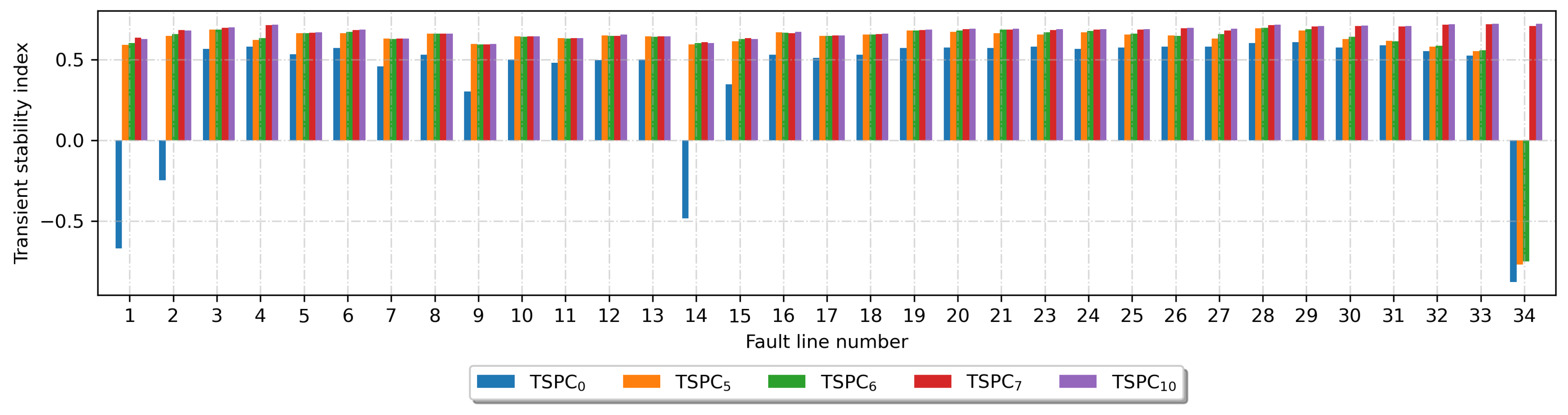
The radar maps and the histogram of TSIs under expected faults with different TSPCs in the New England 10-machine 39-bus system are illustrated in Figure 4 and Figure 5. The radar maps represent the stable domains of different TSPCs.

Before taking TSPC (${\mathrm{TSPC}}_0$), there are four line faults that do not meet the N − 1 stability criterion: ${\mathrm{Line}}_{AC1}$ fault, ${\mathrm{Line}}_{AC2}$ fault, ${\mathrm{Line}}_{AC14}$ fault, and ${\mathrm{Line}}_{AC34}$ fault. After taking ${\mathrm{TSPC}}_7$ and ${\mathrm{TSPC}}_{10}$, all expected faults meet the N − 1 stability criterion, and the stability margin of the power system is improved. However, for ${\mathrm{TSPC}}_5$ and ${\mathrm{TSPC}}_6$, the ${\mathrm{Line}}_{AC34}$ fault cannot meet the N − 1 stability criterion. In general, as the number of controlled objects increases, the TSI under each fault also increases. The TSIs of ${\mathrm{TSPC}}_7$ and ${\mathrm{TSPC}}_{10}$ are similar, indicating that, after taking TSPC measures, the stability of the two operational scenarios is similar. Furthermore, ${\mathrm{TSPC}}_7$ has fewer control objects, which is conducive to the actual generation schedule. Therefore, ${\mathrm{TSPC}}_7$ is selected as the ultimate TSPC on the power system.

The generator rotor angle trajectories under ${\mathrm{Line}}_{AC1}$ fault, ${\mathrm{Line}}_{AC2}$ fault, ${\mathrm{Line}}_{AC14}$ fault, and ${\mathrm{Line}}_{AC34}$ fault, which do not meet the N − 1 stability criterion before taking ${\mathrm{TSPC}}_7$, are illustrated in Figure 6.

For the ${\mathrm{Line}}_{AC1}$ fault, ${\mathrm{Line}}_{AC2}$ fault, ${\mathrm{Line}}_{AC14}$ fault, before taking ${\mathrm{TSPC}}_7$ measures, the rotor angle of generator 10 deviates from other generators and the system becomes unstable. After taking ${\mathrm{TSPC}}_7$ measures, the system can maintain stability after each fault. For the ${\mathrm{Line}}_{AC34}$ fault, before taking ${\mathrm{TSPC}}_7$, the rotor angle of generator 9 deviates from other generators and the system becomes unstable. After taking ${\mathrm{TSPC}}_7$ measures, the power system remains stable after the ${\mathrm{Line}}_{AC34}$ fails.

3.2. IEEE 54-Machine 118-Bus System

3.2.1. Dataset Generation

The dataset of a larger-scale system, the IEEE 54-machine 118-bus system, is generated similar to that of the New England 10-machine 39-bus system in the previous section; 159 AC line faults are included in the pre-defined fault set. An imbalanced dataset of operation conditions is generated, including 7801 stable instances and 196 unstable instances. After implementing the ADASYN technique, a relatively balanced dataset is finally obtained, containing 7801 stable instances and 1408 unstable instances.

3.2.2. Transient Stability Assessment

The TSA models of the IEEE 54-machine 118-bus system are constructed with MLP similarly to those of the New England 10-machine 39-bus system. The performance of the TSA models is shown in

Table 5. Performance of transient stability assessment models in the IEEE 118-bus system.

Type	Accuracy (%)	Precision (%)	Recall (%)	F1_Score (%)	G_Mean (%)
Original	98.2	98.3	99.9	99.1	26.2
Fault information	98.4	98.4	99.9	99.2	37.1
ADASYN	98.8	99.0	98.8	98.9	98.8
Fault information + ADASYN	98.8	98.8	99.8	99.3	96.2

. The proposed TSA model trained by the ADASYN-balanced dataset with fault information has the best performance in accuracy (98.8%) and F1_score (99.3%) and has a good performance in G_mean (96.2%). However, the first two TSA models in Table 5 trained by the dataset without balancing by ADASYN have low G_mean of 26.2% and 37.1% due to the imbalanced data. The proposed TSA model trained by the ADASYN-balanced dataset improves the average accuracy of minority and majority classes for TSA models.

3.2.3. Control Object Determination

A certain operational scenario in the IEEE 54-machine 118-bus system is assumed as an actual current scenario discriminated as unstable by the N − 1 TSA. SHAP is performed on the unstable scenario. The top-15 features with the highest absoluted Shapley values are illustrated in Figure 7.

The interpretation results of SHAP show that the features including $P_{Line109-110}$, $Q_{Line17-113}$, $P_{Line103-110}$, $V{m}_{Bus29}$, etc. contribute a lot to the instability of the scenario. Features, $P_{Line110-112}$ and $P_{Line68-116}$ contribute a lot to the stability of the scenario. In addition, the lines connected to $Bu{s}_{110}$ have the highest absolute Shapley values, indicating that $Bu{s}_{110}$ is an important bus.

In the IEEE 54-machine 118-bus system, 19 of 54 generators, including one frequency modulation generator, output active power to the system, while others only output reactive power. The active power output of these 19 generators is controllable and can be scheduled. Therefore, the importance of active power features of the controllable generators is calculated and ranked, as shown in

Table 6. Importance of controllable features in the IEEE 54-machine 118-bus system.

Feature	$P_{G111}$	$P_{G10}$	$P_{G25}$	$P_{G26}$	$P_{G69}$	$P_{G66}$	$P_{G65}$
${\mathit{I}}_{\mathit{ctrl}}$	0.0586	0.0266	0.0209	0.0179	0.0098	0.0081	0.0076
Feature	$P_{G31}$	$P_{G12}$	$P_{G61}$	$P_{G49}$	$P_{G59}$	$P_{G103}$	$P_{G89}$
${\mathit{I}}_{\mathit{ctrl}}$	0.0073	0.0072	0.0071	0.0068	0.0064	0.0054	0.0048
Feature	$P_{G46}$	$P_{G80}$	$P_{G87}$	$P_{G54}$	$P_{G100}$
${\mathit{I}}_{\mathit{ctrl}}$	0.0040	0.0039	0.0038	0.0037	0.0022

.

In general, the number of control objects, m, can be determined by operators when applied to the practical power systems. In the simulation analysis, m is set as 0, 9, 14, and 19 to display the feasibility of the proposed method.

3.2.4. Control Amount Determination

Within the control scope obtained in the previous section, TSCOPF is solved by DE to obtain the control amount of TSPC in this section. Take ${\mathrm{TSPC}}_m$ as different operational schedules of the IEEE 54-machine 118-bus system, including the initial operation condition (${\mathrm{TSPC}}_0$).

The results of DE-TSCOPF in different control strategies are shown in Figure 8. The operation costs of ${\mathrm{TSPC}}_0$, ${\mathrm{TSPC}}_9$, ${\mathrm{TSPC}}_{14}$, and ${\mathrm{TSPC}}_{19}$ are 135,128.39 $/h, 133,252.34 $/h, and 131,161.24 $/h, respectively. For the IEEE 54-machine 118-bus system, the operation cost increases slightly after TSPC as the number of control objects increases.

The stable domains of different TSPCs in the IEEE 54-machine 118-bus system are shown in Figure 9. The TSI of the no. 159 fault (the fault on ${\mathrm{Line}}_{76-118}$) is −0.83 in ${\mathrm{TSPC}}_0$. That means the system would be unstable once it suffers from the no. 159 fault. Other faults are safe. After taking the TSPCs, the TSI of the no. 159 fault is increased significantly, for example, from −0.83 to 0.49 after taking ${\mathrm{TSPC}}_{14}$.

The averages of TSIs under the ${\mathrm{TSPC}}_0$, ${\mathrm{TSPC}}_9$, ${\mathrm{TSPC}}_{14}$, and ${\mathrm{TSPC}}_{19}$ are 0.644, 0.628, 0.704, and 0.705, respectively. When the number of controllable generators is nine, which is minor, the average TSI may be less than that without TSPC. That is because, in ${\mathrm{TSPC}}_9$, the safety margins of some faults are sacrificed due to the limit of control, thus ensuring that the system is a secure state under any fault circumstance. The scarification is acceptable because it maintains the system security.

The security of the system is reinforced as the number of controlled generators increases. However, when the number exceeds a certain amount, the reinforcement is somewhat limited. Control strategies with fewer generators to be adjusted are recommended. The proposed method provides a possible way to narrow the number of controlled generators and improves the convenience of operation and the precision of preventive control. The power system dispatchers should consider the trade-off between the convenience of the implementation and the security of systems, which can be further determined according to optional and specific objectives.

The generator rotor angle trajectories under the no. 2 fault (the Line_1–3 fault) and the no. 159 fault (the Line_76–118 fault) before and after taking TSPC₁₄ are illustrated in Figure 10. For the Line_1–3 fault, before taking TSPC₁₄ measures, the rotor angle of G1 deviates very much from other generators in the first oscillation period. After taking TSPC₁₄ measures, the oscillation amplitude of the rotor angle of G1 is reduced and the system can maintain a relatively high stability margin after each fault. For the Line_76–118 fault, before taking TSPC₁₄, the rotor angle of G76 deviates from other generators and the system becomes unstable. After taking TSPC₁₄ measures, the power system remains stable after the Line_76–118 fails.

3.2.5. Time Performance

The time cost of the proposed method mainly covers the interpretation time and the TSCOPF time. The time consumption of SHAP interpretation is related to the number of input features and the number of background data for the calculation of Shapley values. For the training data of the IEEE 54-machine 118-bus system, the number of input features is 919 and the number of initial training data is 7367. K-means++ algorithm is introduced to cluster the initial large amounts of data and to reduce the background data to K. The sum of squared distances (SSD) of samples to their closest cluster center is used as the clustering performance index. The smaller the sum of squared distances, the better the clustering performance. The elapsed time of interpretation and the clustering performance of k-means++ with different K are tested and illustrated in Figure 11.

As K increases, the sum of squared distances of data decreases, and the time elapsed for pure clustering and the total time for clustering and SHAP increase. If the background data exceed 140, the run time slows down sharply due to insufficient allocated memory. It is suggested that the clustering approach be used to aggregate the background data into less than 100 samples.

Furthermore, the time consumptions of DE-TSCOPF of ${\mathrm{TSPC}}_9$, ${\mathrm{TSPC}}_{14}$, and ${\mathrm{TSPC}}_{19}$ are 56.453 s, 59.483 s, and 58.843 s. They are within a minute, which satisfies the time requirement of online preventive control for the power system in such a size. Note that the proposed method of accurately narrowing the control objects is generalized and is suitable for most TSCOPF approaches. Other TSCOPF approaches can be selected or improved to reduce the time consumptions of TSPC further.

4. Conclusions

A model interpretation-based multi-contingency coordinated preventive control optimization strategy, adaptive to the scenarios of multiple generators and multiple contingencies, is proposed in this paper. In the proposed strategy, an augmented balanced dataset is constructed by covering fault information and using the ADASYN technique. The proposed TSA machine learning model has a better performance than the original model both in accuracy and in the G_mean index. In addition, the proposed model is suitable for stability judgment under all anticipated faults in power systems. The model interpretation mechanism is used to narrow the scope of preventive control objects and realizes the control and economic optimization of generation scheduling under the premise of ensuring system stability. Through k-means++ clustering, the background data can be summarized into a small but representative dataset, which improves the feasibility and practicability of SHAP interpretation.

Besides differential evolution used in this paper, other approaches to solving optimization problems can also be applied to the proposed preventive control strategy. Due to the feasibility of the model interpretation mechanism, the proposed optimization method can be easily extended to other applications such as voltage stability or available transfer capability. Furthermore, the high penetration of renewable sources, including wind power generation and photovoltaic systems, increased the operational uncertainty of power systems. Therefore, TSA and TSPC strategies under renewable sources are exciting, which will be our future works.

References

- Hassan, R.; Li, C.; Liu, Y. Online dynamic security assessment of wind integrated power system using SDAE with SVM ensemble boosting learner. Int. J. Electr. Power Energy Syst. 2021, 125, 106429. [Google Scholar] [CrossRef]
- Yuan, H.; Xu, Y. Trajectory sensitivity based preventive transient stability control of power systems against wind power variation. Int. J. Electr. Power Energy Syst. 2020, 117, 105713. [Google Scholar] [CrossRef]
- Sharifzadeh, H.; Amjady, N.; Zareipour, H. Multi-period stochastic security-constrained OPF considering the uncertainty sources of wind power, load demand and equipment unavailability. Electr. Power Syst. Res. 2017, 146, 33–42. [Google Scholar] [CrossRef]
- Bhui, P.; Senroy, N. Real-Time Prediction and Control of Transient Stability Using Transient Energy Function. IEEE Trans. Power Syst. 2017, 32, 923–934. [Google Scholar] [CrossRef]
- Passaro, M.C.; da Silva, A.P.A.; Lima, A.C.S. Preventive Control Stability Via Neural Network Sensitivity. IEEE Trans. Power Syst. 2014, 29, 2846–2853. [Google Scholar] [CrossRef]
- Momoh, J.; Koessler, R.; Bond, M.; Stott, B.; Sun, D.; Papalexopoulos, A.; Ristanovic, P. Challenges to optimal power flow. IEEE Trans. Power Syst. 1997, 12, 444–455. [Google Scholar] [CrossRef] [Green Version]
- Condren, J.; Gedra, T. Expected-Security-Cost Optimal Power Flow With Small-Signal Stability Constraints. IEEE Trans. Power Syst. 2006, 21, 1736–1743. [Google Scholar] [CrossRef]
- Canizares, C.; Rosehart, W.; Berizzi, A.; Bovo, C. Comparison of voltage security constrained optimal power flow techniques. In Proceedings of the 2001 Power Engineering Society Summer Meeting, Conference Proceedings (Cat. No.01CH37262), Vancouver, BC, Canada, 15–19 July 2001; Volume 3, pp. 1680–1685. [Google Scholar] [CrossRef]
- Xu, Y.; Yin, M.; Dong, Z.Y.; Zhang, R.; Hill, D.J.; Zhang, Y. Robust Dispatch of High Wind Power-Penetrated Power Systems Against Transient Instability. IEEE Trans. Power Syst. 2018, 33, 174–186. [Google Scholar] [CrossRef]
- Nguyen, T.; Pai, M. Dynamic security-constrained rescheduling of power systems using trajectory sensitivities. IEEE Trans. Power Syst. 2003, 18, 848–854. [Google Scholar] [CrossRef] [Green Version]
- Xu, Y.; Dong, Z.Y. Trajectory sensitivity analysis on the equivalent one-machine-infinite-bus of multi-machine systems for preventive transient stability control. IET Gener. Transm. Distrib. 2015, 9, 276–286. [Google Scholar] [CrossRef]
- Mo, N.; Zou, Z.Y.; Chan, K.W.; Pong, T. Transient stability constrained optimal power flow using particle swarm optimisation. IET Gener. Transm. Distrib. 2007, 1, 476–483. [Google Scholar] [CrossRef]
- Abhyankar, S.; Geng, G.; Wang, X.; Dinavahi, V. Solution techniques for transient stability-constrained optimal power flow—Part I. IET Gener. Transm. Distrib. 2017, 11, 3177–3185. [Google Scholar] [CrossRef]
- Geng, G.; Abhyankar, S.; Wang, X.; Dinavahi, V. Solution techniques for transient stability-constrained optimal power flow—Part II. IET Gener. Transm. Distrib. 2017, 11, 3186–3193. [Google Scholar] [CrossRef]
- Wu, D.; Gan, D.; Jiang, J.N. An improved micro-particle swarm optimization algorithm and its application in transient stability constrained optimal power flow. Eur. Trans. Electr. Power 2014, 24, 395–411. [Google Scholar] [CrossRef]
- Zhang, X.; Dunn, R.; Li, F. Stability constrained optimal power flow for the balancing market using genetic algorithms. In Proceedings of the 2003 IEEE Power Engineering Society General Meeting (IEEE Cat. No.03CH37491), Toronto, ON, Canada, 13–17 July 2003; Volume 2, pp. 932–937. [Google Scholar] [CrossRef]
- Chan, K.; Chan, K.; Ling, S.; Iu, H.; Pong, G. Solving multi-contingency transient stability constrained optimal power flow problems with an improved GA. In Proceedings of the 2007 IEEE Congress on Evolutionary Computation, Singapore, 25–28 September 2007; pp. 2901–2908. [Google Scholar] [CrossRef]
- Kucuktezcan, C.F.; Gene, V.M.I. A new dynamic security enhancement method via genetic algorithms integrated with neural network based tools. Electr. Power Syst. Res. 2012, 83, 1–8. [Google Scholar] [CrossRef]
- Ye, C.J.; Huang, M.X. Multi-Objective Optimal Power Flow Considering Transient Stability Based on Parallel NSGA-II. IEEE Trans. Power Syst. 2015, 30, 857–866. [Google Scholar] [CrossRef]
- Cai, H.R.; Chung, C.Y.; Wong, K.P. Application of Differential Evolution Algorithm for Transient Stability Constrained Optimal Power Flow. IEEE Trans. Power Syst. 2008, 23, 719–728. [Google Scholar] [CrossRef]
- Chen, Y.; Luo, F.; Xu, Y.; Qiu, J. Self-adaptive differential approach for transient stability constrained optimal power flow. IET Gener. Transm. Distrib. 2016, 10, 3717–3726. [Google Scholar] [CrossRef]
- Ledesma, P.; Calle, I.A.; Castronuovo, E.D.; Arredondo, F. Multi-contingency TSCOPF based on full-system simulation. IET Gener. Transm. Distrib. 2017, 11, 64–72. [Google Scholar] [CrossRef] [Green Version]
- Pizano-Martinez, A.; Fuerte-Esquivel, C.R.; Ruiz-Vega, D. Global Transient Stability-Constrained Optimal Power Flow Using an OMIB Reference Trajectory. IEEE Trans. Power Syst. 2010, 25, 392–403. [Google Scholar] [CrossRef]
- Pizano-Martinez, A.; Fuerte-Esquivel, C.R.; Ruiz-Vega, D. A New Practical Approach to Transient Stability-Constrained Optimal Power Flow. IEEE Trans. Power Syst. 2011, 26, 1686–1696. [Google Scholar] [CrossRef]
- Jiang, Q.; Huang, Z. An Enhanced Numerical Discretization Method for Transient Stability Constrained Optimal Power Flow. IEEE Trans. Power Syst. 2010, 25, 1790–1797. [Google Scholar] [CrossRef]
- Jiang, Q.; Geng, G. A Reduced-Space Interior Point Method for Transient Stability Constrained Optimal Power Flow. IEEE Trans. Power Syst. 2010, 25, 1232–1240. [Google Scholar] [CrossRef]
- Francisco, A.; Pablo, L.; Daniel, C.E. Optimization of the operation of a flywheel to support stability and reduce generation costs using a Multi-Contingency TSCOPF with nonlinear loads. Int. J. Electr. Power Energy Syst. 2019, 104, 69–77. [Google Scholar]
- Arredondo, F.; Ledesma, P.; Castronuovo, E.D.; Aghahassani, M. Stability Improvement of a Transmission Grid with High Share of Renewable Energy using TSCOPF and Inertia Emulation. IEEE Trans. Power Syst. 2020. [Google Scholar] [CrossRef]
- Xu, Y.; Dong, Z.Y.; Meng, K.; Zhao, J.H.; Wong, K.P. A Hybrid Method for Transient Stability-Constrained Optimal Power Flow Computation. IEEE Trans. Power Syst. 2012, 27, 1769–1777. [Google Scholar] [CrossRef]
- Pizano-Martinez, A.; Fuerte-Esquivel, C.R.; Zamora-Cárdenas, E.A.; Lozano-García, J.M. Directional Derivative-Based Transient Stability-Constrained Optimal Power Flow. IEEE Trans. Power Syst. 2017, 32, 3415–3426. [Google Scholar] [CrossRef]
- Miranda, V.; Fidalgo, J.; Lopes, J.; Almeida, L. Real time preventive actions for transient stability enhancement with a hybrid neural network-optimization approach. IEEE Trans. Power Syst. 1995, 10, 1029–1035. [Google Scholar] [CrossRef]
- Fidalgo, J.; Pecas Lopes, J.; Miranda, V. Neural networks applied to preventive control measures for the dynamic security of isolated power systems with renewables. IEEE Trans. Power Syst. 1996, 11, 1811–1816. [Google Scholar] [CrossRef]
- Tangpatiphan, K.; Yokoyama, A. Evolutionary Programming Incorporating Neural Network for Transient Stability Constrained Optimal Power Flow. In Proceedings of the 2008 Joint International Conference on Power System Technology and IEEE Power India Conference, New Delhi, India, 12–15 October 2008; pp. 1–8. [Google Scholar] [CrossRef]
- Gutierrez-Martinez, V.J.; Cañizares, C.A.; Fuerte-Esquivel, C.R.; Pizano-Martinez, A.; Gu, X. Neural-Network Security-Boundary Constrained Optimal Power Flow. IEEE Trans. Power Syst. 2011, 26, 63–72. [Google Scholar] [CrossRef]
- He, H.; Bai, Y.; Garcia, E.A.; Li, S. ADASYN: Adaptive synthetic sampling approach for imbalanced learning. In Proceedings of the 2008 IEEE International Joint Conference on Neural Networks (IEEE World Congress on Computational Intelligence), Hong Kong, China, 1–8 June 2008; pp. 1322–1328. [Google Scholar]
- Strumbelj, E.; Kononenko, I. A general method for visualizing and explaining black-box regression models. In Proceedings of the 10th International Conference on Adaptive and Natural Computing Algorithms(ICANNGA), Ljubljana, Slovenia, 14–16 April 2011; pp. 21–30. [Google Scholar]
- Arthur, D.; Vassilvitskii, S. K-means++: The advantages of careful seeding. In Proceedings of the 18th ACM-SIAM Symposium on Discrete Algorithms, New Orleans, LA, USA, 7–9 January 2007; pp. 1027–1035. [Google Scholar]
- Storn, R.; Price, K. Differential Evolution: A Simple and Efficient Adaptive Scheme for Global Optimization Over Continuous Spaces. J. Glob. Optim. 1997, 11, 341–359. [Google Scholar] [CrossRef]
Figure 1.
Framework of the proposed method.
Figure 2.
Single line diagram of the New England 10-machine 39-bus system.
Figure 3.
SHAP interpretation of an unstable scenario in the New England 39-bus system.
Figure 4.
Stability domains after different TSPCs in the New England 10-machine 39-bus system.
Figure 5.
Histogram of TSIs under different faults after different TSPCs in the New England 10-machine 39-bus system.
Figure 6.
Angle trajectories of generators before and after taking in the New England 10-machine 39-bus system.
Figure 7.
SHAP interpretation of an unstable scenario in the IEEE 54-machine 118-bus system.
Figure 8.
Generator output changes with respect to the initial schedule in the the IEEE 54-machine 118-bus system.
Figure 9.
Stability domain-type TSIs after different TSPCs in the IEEE 54-machine 118-bus system.
Figure 10.
Angle trajectories of generators before and after taking in the IEEE 54-machine 118-bus system under (a) the Line1–3 fault and (b) the Line76–118 fault.
Figure 11.
Clustering performance of k-means with different values of K in the IEEE 54-machine 118-bus system.