Machine Learning-Based Identification Strategy of Fuel Surrogates for the CFD Simulation of Stratified Operations in Low Temperature Combustion Modes

Abstract

Many researchers in industry and academia are showing an increasing interest in the definition of fuel surrogates for Computational Fluid Dynamics simulation applications. This need is mainly driven by the necessity of the engine research community to anticipate the effects of new gasoline formulations and combustion modes (e.g., Homogeneous Charge Compression Ignition, Spark Assisted Compression Ignition) to meet future emission regulations. Since those solutions strongly rely on the tailored mixture distribution, the simulation and accurate prediction of the mixture formation will be mandatory. Focusing purely on the definition of surrogates to emulate liquid phase and liquid-vapor equilibrium of gasolines, the following target properties are considered in this work: density, Reid vapor pressure, chemical macro-composition and volatility. A set of robust algorithms has been developed for the prediction of volatility and Reid vapor pressure. A Bayesian optimization algorithm based on a customized merit function has been developed to allow for the efficient definition of surrogate formulations from a palette of 15 pure compounds. The developed methodology has been applied on different real gasolines from literature in order to identify their optima surrogates. Furthermore, the ‘unicity’ of the surrogate composition is discussed by comparing the optimum solution with the most different one available in the pool of equivalent-valuable solutions. The proposed methodology has proven the potential to formulate surrogates characterized by an overall good agreement with the target properties of the experimental gasolines (max relative error below 10%, average relative error around 3%). In particular, the shape and the end-tails of the distillation curve are well captured. Furthermore, an accurate prediction of key chemical macro-components such as ethanol and aromatics and their influence on evaporative behavior is achieved. The study of the ‘unicity’ of the surrogate composition has revealed that (i) the unicity is strongly correlated with the accuracy and that (ii) both ‘unicity’ and accuracy of the prediction are very sensitive to the high presence of aromatics.

1. Introduction

Nowadays the need to reduce the fossil fuel consumption and to accomplish the increasingly stringent emissions standard required to place gasoline-powered vehicles on market is leading to dramatical changes in the framework of internal combustion engines. In the last decades Direct Injection Spark Ignition (DISI) engines have become a well-established technology to fulfill fuel economy and tailpipe emissions thanks to support devices and strategies such as downsized turbo-engines, increasing injection pressure (300–400 bar are available in the current market, 700 bar can be achieved for specific applications e.g., the Magneti Marelli injection system implemented in the Mazda’s Skyactiv-X [1]). However, nitrogen oxides (NOx) emissions and engine efficiency remain a concern strictly connected to the use of classical spark plug devices. In this scenario, advanced combustion concepts named Low-Temperature Combustion (LTC) modes are gaining attention as a solution to reach both emissions target and fuel economy goals at low and medium engine load. Under LTC modes the engine is characterized by a highly dilute environment, and the combustion is fully or mainly driven by the multi-point no-knock auto-ignition of the gasoline as described by chemical kinetics simulations. The high degree of dilution and the lack of the spark device promote low temperature combustion events that allow reduced soot and NOx emissions. Furthermore, the low temperature strongly reduces heat losses, resulting in higher engine efficiency [2].

Examples of promising gasoline LTC solutions are Homogeneous Charge Compression Ignition (HCCI) and Spark Assisted Compression Ignition (SACI). Giving a brief view of these concepts: (i) in HCCI a diluted and homogeneous environment is created, then the mixture ignites by compression heating thanks to inlet temperature control and compression ratios higher than that of classical Spark Ignition (SI) engines; (ii) SACI multi-mode combustion is a bridge between HCCI and SI operations, a spark device is used to directly control the ignition timing initiating a flame front whose propagation is responsible for the compression and the heating up of the end-gases. The following formation of local auto-ignition spots near the flame front promotes the Compression Ignition (CI) of the fresh mixture. Despite the advantages of those LTC modes, the limited load range and the abrupt in-cylinder heat release rate and pressure rise rate remain a concern. Among different solutions adopted to approach those technical issues, fuel stratification has shown a great potential. In [3] Sjöberg and Dec conducted experiments on a modified Diesel engine operated in HCCI mode with different gasoline-like mixtures. The fuel stratification was applied by means of two direct injection events with different timing for the second injection. The experiments showed that a tailored stratification is capable to extend HCCI operations to higher loads with a well balance between NOx emissions and pressure rise rate. Furthermore, the Authors showed that the use of fuel mixtures with two-stage ignition behavior strongly enhances the benefits of fuel stratification. In [4] Priyadarshini et al., performed Computational Fluid Dynamics (CFD) simulations of the same HCCI engine used in [3]. A E10 (10% vol. ethanol addition) gasoline blend was stratified by means of two injection events, then different timings for the second injection were tested. The stratification of temperature was observed as a consequence of the mixture stratification due to the latent heat of vaporization of the fuel. The Authors described fuel stratification as an effective control strategy of the in-cylinder heat release rate. It was also highlighted that tailored optimization of fuel stratification leads to advanced combustion phasing, increased thermal efficiency, reduced pressure rise rate and NOx emissions. In the comprehensive work of Zhou et al. [5] experiments were carried out under SI, HCCI and SACI modes with the same test engine. The Authors achieved fuel stratification by adopting different injection timings. The Authors reported that fuel stratification helps to suppress knock events in the end-gas and to mitigate the burn rate, resulting in smoother HCCI (low load)–SACI (medium load) transitions and SACI (medium load)–SI (high load) transitions. Moreover, fuel stratification under SACI operations enables stable combustions richer in EGR (Exhaust Gas Recirculation) and more anticipated spark timings. It must be underlined that in current DISI engines as well, fuel stratification has shown the capability to stabilize ultra-lean operations and to be a lever for knock control and mitigation [6].

As far as lean low temperature combustions are concerned, low and medium load operations in the next generation engines will be dramatically sensitive to the three-dimensional distribution of the mixture. As a consequence, the accurate prediction of the evaporative behavior of new gasoline blends will be fundamental. Nowadays, three-dimensional CFD engine simulation is an acknowledged technique to support and address the engine development and, to assess new scenarios. It must be remembered that commercial gasolines are complex mixtures of hundreds of species whose full reproduction in CFD simulations is not available because their exact composition is not known and even so, the time spent for the tracing and resolution of that number of species would be unaffordable. Therefore, the common practice is the representation of real gasolines by means of surrogates, namely mixtures of different well characterized pure components. The number and type of the pure components comprised in the surrogate strongly depend on which aspects of the real gasoline are under analysis.

In the current literature the study of algorithms for the design of comprehensive fuel surrogates for practical gasolines is widely discussed. Most of the published works (e.g., [7,8,9,10,11]) are focused on the use of different searching techniques e.g., regression models and genetic algorithms, for the formulation of surrogates capable to mimic the chemical aspects or both chemical and physical aspects of real gasolines. It must be underlined that, as reported in [12], the latter approach suffers from the current poor chemical kinetics characterization of different essential pure compounds, for which kinetic mechanisms need to be developed and validated yet. On the other hand, a wide number of reliable physical properties of the same pure compounds are commonly available. As shown by literature results [7,8,9,10,11] the mimic of physical and chemical properties at the same time with a single surrogate is extremely complex regardless of the searching strategy. In [7,8,9,10,11] the Authors achieved surrogates with values of liquid density, carbon-to-hydrogen ratio, chemical composition in reasonable agreement with experimental data while poor representations of the end-tails of the distillation curve and octane rating were presented. To the best knowledge of the present Authors, a very few works have approached the fuel surrogate formulation by using machine learning techniques or by placing emphasis on only the physical properties. In [13] Pati et al., adopted a genetic algorithm to search surrogates representative of the distillation and vapor pressure curves of four gasolines with different levels of ethanol blending. Two different sizes of the initial palette were tested, and surrogates comprising 5 and 7 components were achieved. The results showed that the proposed methodology was capable to capture with reasonable accuracy the vapor pressure curve and the early distillation behavior (20% to 40% distilled volume). However, significant mismatches were reported for the very early distillation behavior (0% to 10% distilled volume) and for values in the right end-tail of the distillation curve, indeed, temperature differences between 10–25 °C were detected in those ranges. In [14] Muelas et al., aimed to capture the evaporative behavior and the soot tendency of a reference heating oil representative of the physicochemical complexity of fuels. A multi-objective regression algorithm was used to capture liquid density, carbon-to-hydrogen ratio, molecular weight, soot tendency and distillation curve by means of 2-components surrogates. Errors around 15% were detected in reproducing distillation curve, soot tendency and molecular weight likely due to the complexity of the multi-property optimization associated to the 2-component approximation. In [15] Zhu et al., applied a Bayesian multi kernel learning model to define surrogates capable to predict the soot tendency of fuels based on an in-house developed extensive experimental database. The work was focused on jet, diesel and bio-diesel fuels. The soot tendency of the surrogates presented by the Authors were in line with experiments, indeed coefficients of correlation over 0.95 were reported.

It must be underlined that according to the standard industrial practice in three-dimensional CFD engine simulation, two different gasoline surrogates can be used during the same calculation: (i) firstly, a n1-components surrogate is adopted to simulate the mixture formation i.e., spray formation, spray evaporation, spray-wall impingement, liquid film evaporation; (ii) then, the spatial distributions of pressure, temperature and mixture are given as input to correlations or models for laminar flame speed and ignition-delay time whose tuning parameters are taken from the chemical kinetic simulation of a different n2-components surrogate designed to simulate the combustion behavior of the same gasoline.

This work proposes an advanced in-house developed machine-learning based methodology to define fuel surrogates capable to mimic the evaporative properties of nowadays gasoline blends. The components of the surrogate are selected from a palette of 15 pure compounds carefully chosen by the present Authors after a literature review. A Bayesian algorithm is trained to provide the user with a multi-component fuel mixture representative of the evaporative behavior of the target fuel. The provided composition can be implemented in CFD codes when the liquid fuel spray setup is required in the pre-processing phase. The algorithm performs a multi-objective optimization considering two types of constraints: (i) primary constraints, which are the fuel properties that the code aims to pursue during the optimization task; (ii) secondary or light constraints, which are fuel properties that are not included in the multi-objective task, instead they simply must fall in an acceptability range with respect to experimental value. In this work the primary constraints (optimization targets) are liquid density, Reid Vapor Pressure (RVP), volatility (distillation TX, temperature at X% recovered volume), chemical composition. Research Octane Number (RON) and Motor Octane Number (MON) are used as light constraints. The experimental data of four different gasolines from literature are used as validation benchmark. As mentioned before, published works focused on techniques to design surrogates capturing liquid and liquid-vapor equilibrium physical properties are quite rare in the current literature. Moreover, in the few works that have approached the present topic, the fuel properties emulation by surrogate formulation is not in line with the current accuracy requirements from modeling. Besides investigating a rare topic with greater accuracy and increased complexity with respect to similar literature works, the original contribution of the present work is the use novel advanced techniques such as Bayesian machine learning algorithms instead of common practice regression models and genetic algorithms. Moreover, in contrast to literature works [7,8,9,10,11], the novelty revealed by the present methodology is the potential to define surrogates capable to capture both physical properties (distillation behavior, vapor pressure, density) and chemical information (RON, MON, composition) at the same time with almost the same accuracy. It is remembered that most of literature works are focused on the formulation of surrogates for Fuels for Advanced Combustion Engines (FACE) gasolines, whose octane rating was strongly lower than that of nowadays blends. Therefore, it is worthwhile that the present Authors have tested the methodology with success on nowadays high-octane rating gasolines, for which the simultaneous match of RON, MON and physical properties is more complex. A further original contribution of the present work is the here called ‘unicity analysis’, which consists in the comparison between the optimum surrogate and the surrogate in the same solution pool that differs the most by the optimum formulation, with the aim to assess if an almost unique composition is allowed. Otherwise, the characteristics of the real fuel that affect the composition variability of possible surrogates is studied and the sensitivity of the target properties to the variability is analyzed. The current literature lacks of analyses of that type and the results are expected to be helpful for the improvement of the present methodology and the development of new ones by increasing the knowledge in addressing the searching process towards specific subsets of the exploration space.

2. Methodology

2.1. Base Palette

After a review of gas chromatography data in findings regarding gasolines for light duty application, a palette of 15 pure substances comprising one oxygenate, four n-paraffins, two i-paraffins, two olefins, two cycloalkanes and four aromatics was considered. The compounds and a set of their representative properties including liquid density (ρ), vapor pressure (p_V), boiling temperature (T_b), RON, MON, are listed in

Table 1. Palette of the selected pure compounds and their properties.

Compound	Class	ρ @20 °C (kg/m3)	pV @20 °C (kPa)	Tb (°C)	RON	MON
Ethanol	Alcohols	791	5.85	351.5	109	90
n-Pentane	n-Paraffins	627	56.3	309.4	62	62
n-Hexane	n-Paraffins	661	16.1	342.1	19	26
n-Heptane	n-Paraffins	686	4.67	371.5	0	0
n-Decane	n-Paraffins	732	0.12	447.1	-41	-15
i-Pentane	i-Paraffins	622	76.2	301	93.5	62
i-Octane	i-Paraffins	695	5.11	372.4	100	100
1-Pentene	Olefins	641	70.1	303	91	77
1-Hexene	Olefins	674	19.2	336.5	76	63.4
Cyclopentane	Naphthenes	746	34.4	322.1	101	84.9
Cyclohexane	Naphthenes	778	10.3	353.1	83	85
Toluene	Aromatics	869	2.9	383.9	116	103.5
m-Xylene	Aromatics	865	0.83	412.1	118	115
Ethylbenzene	Aromatics	868	0.57	409.3	101	98
1,2,4-trimethylbenzene	Aromatics	876	0.20	441.1	111	124

. Liquid density, vapor pressure and boiling temperature are taken from [16], values of RON and MON from [17] and [18], respectively.

2.2. Optimization Targets and Their Modeling

As pointed out in 1., the formulation of a proper gasoline surrogate depends on which characteristics of the real gasoline are needed. Since the main focus of this work is the reproduction of the evaporative behavior of nowadays gasolines, the following properties are selected as targets (primary constraints) for the multi-objective optimization task: (1) macroscopic chemical composition, given as EPIONA (Ethanol, n-Paraffins, i-Paraffins, Olefins, Naphthenes, Aromatics) volumetric composition; (2) liquid density (ρ) at 15 °C; (3) a selection of distillation curve data, namely temperatures from T10 to T90 with steps of 10% distilled volume; (4) the Reid Vapor Pressure. As described in the last paragraph on 1., RON and MON values are used as light constraints to check that the defined surrogates can be representative of nowadays octane rating. Further details on the use of RON and MON values are given in Section 2.3.

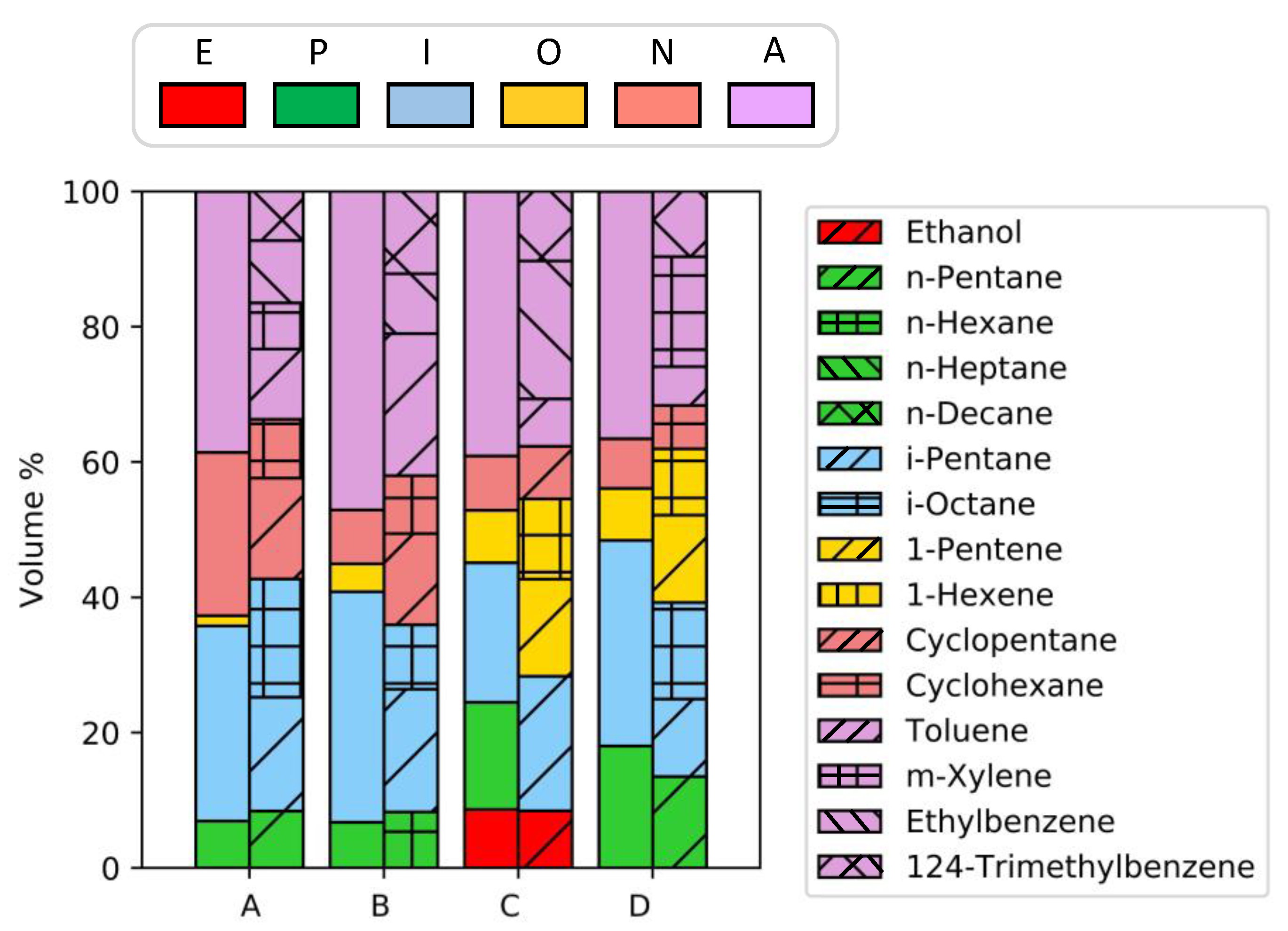
2.2.1. Macroscopic Chemical Composition

As mentioned before, the macroscopic chemical composition of the surrogate is given by the EPIONA volumetric composition. Once the surrogate attempt has been formulated, EPIONA is directly calculated from the composition of the latter as the sum of the volumetric contribution of each component to the corresponding chemical class (Ethanol, n-Paraffin, i-Paraffin, Olefin, Naphthene, Aromatic).

2.2.2. Liquid Density

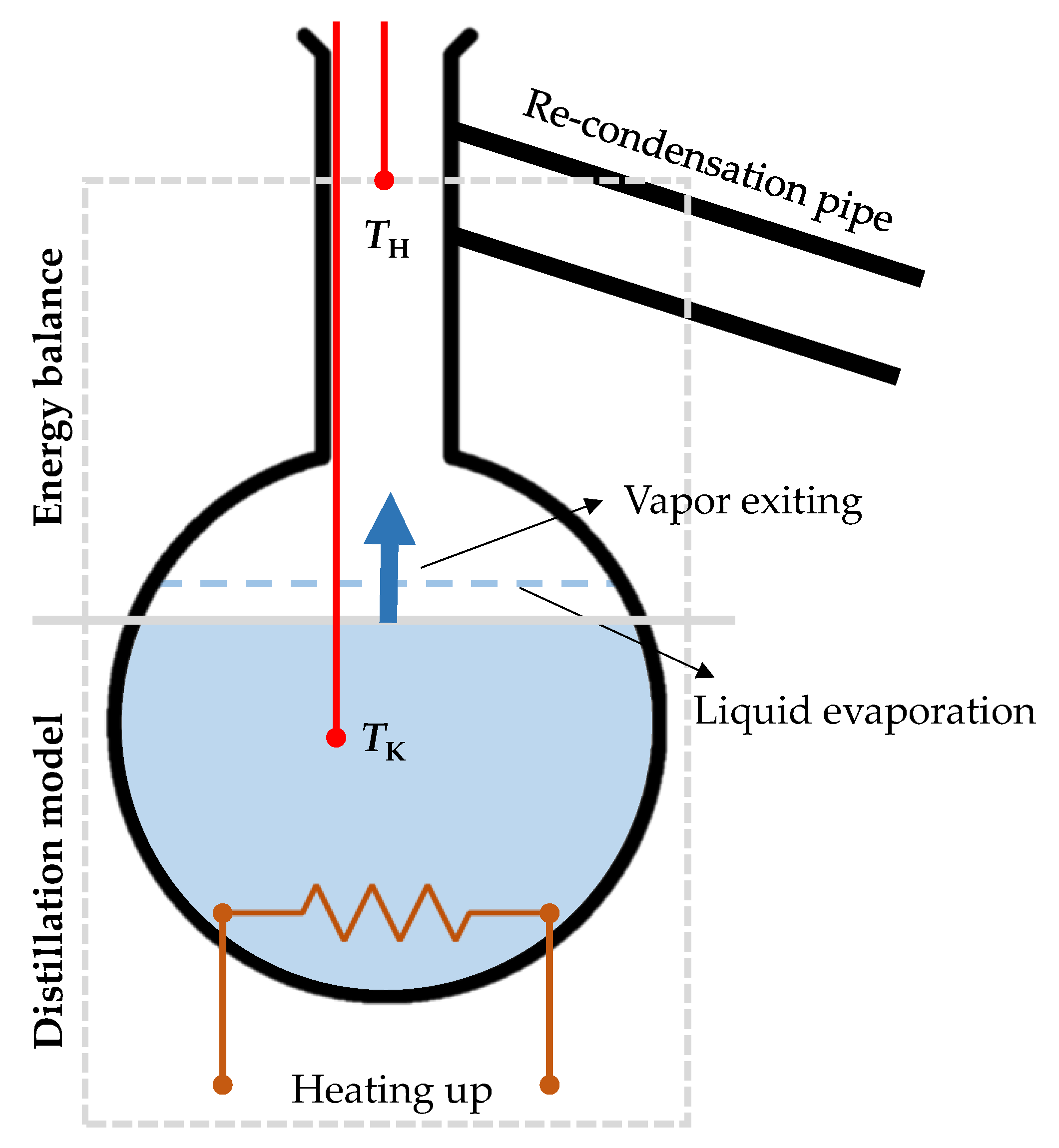
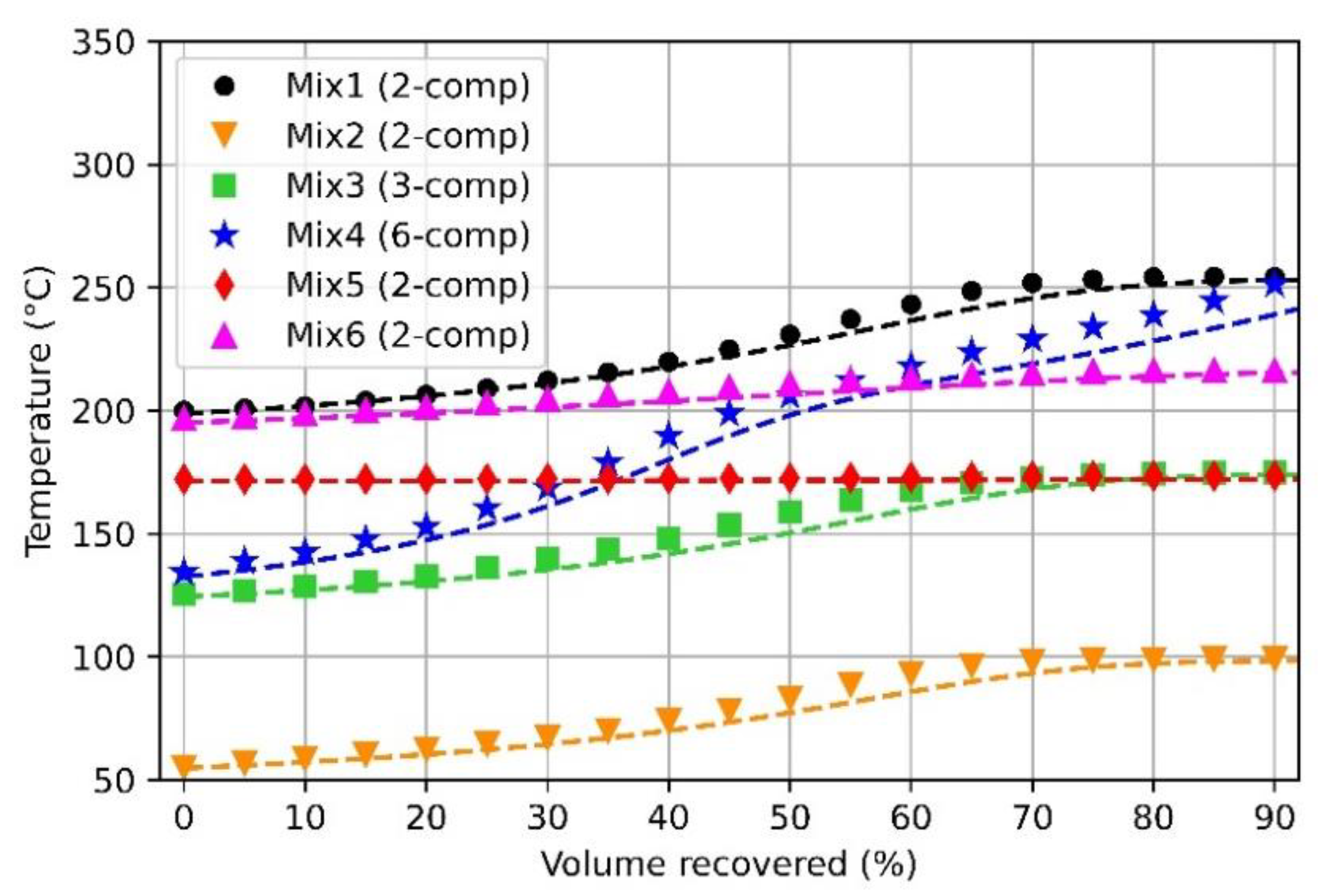
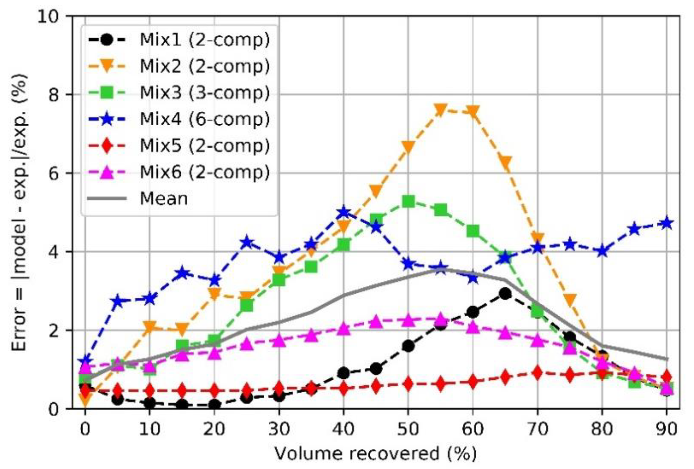
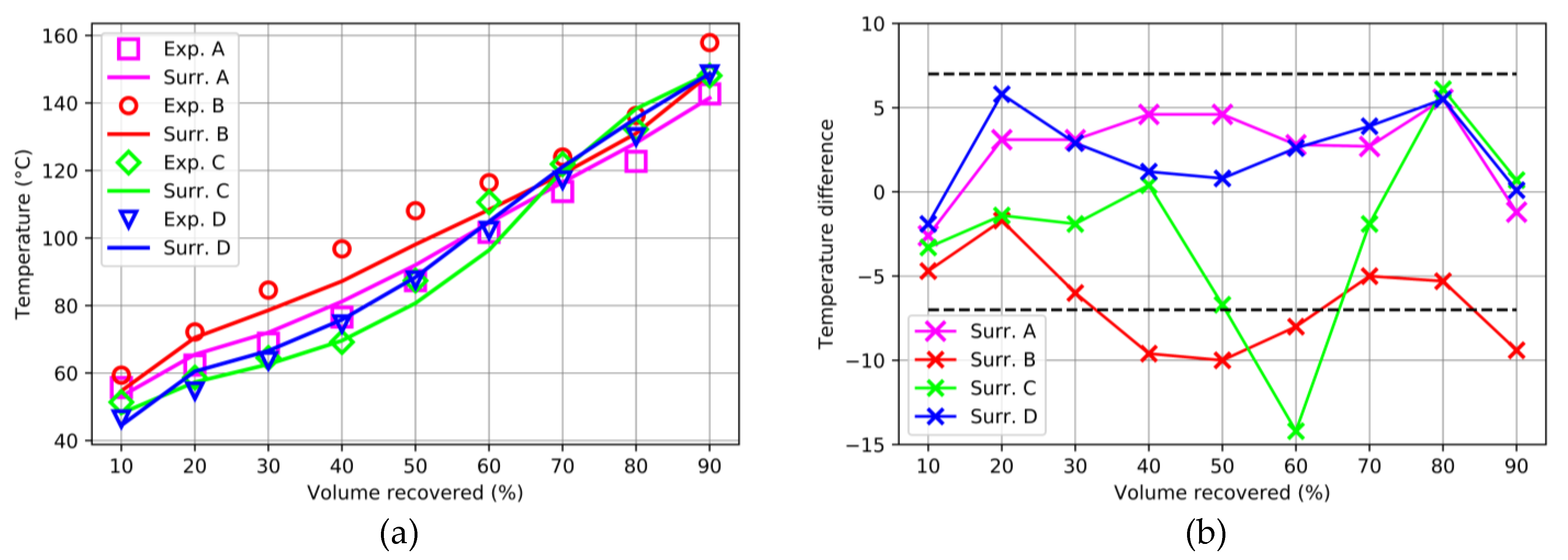
The density of the surrogate mixture is calculated by means of the mass weighted average of the density values of each component. The density of the pure compounds is estimated according to the temperature-dependent correlations in [16] at 15 °C.

2.2.3. Volatility

Since evaporation properties are not additive, the calculation of distillation data and the RVP required dedicated sub-models. Based on the works of Slavinskaya et al. [19] and Abianeh et al. [20] the present Authors developed a zero-dimensional three steps distillation model in Python-3 environment. The model is provided with the surrogate composition and returns the distillate temperature both at the bottom of the kettle (in the liquid phase), which is called kettle distillation temperature (T_K, Figure 1), and at the top of the kettle before the re-condensation pipe, which is called head distillation temperature (T_H, Figure 1). The vapor re-condensation that may occur in the kettle neck was neglected.

The mentioned three steps of the model are: (1) modelling of the first boiling temperature (T0) by means of a pure thermodynamic model; (2) modelling of the distillation process (T0 < TX ≤ T90) by coupling the same abovementioned pure thermodynamic model with a mathematical model of no-reflux simple batch distillation operations; (3) application of the energy balance to determine the head distillation temperature from the kettle distillation temperature. It must be underlined that most of the experimental distillation rigs record only the head distillation temperature since the measure of the kettle distillation temperature is quite complex due to the position of the thermocouple, which is affected by the continuous phase change. Therefore, the third modeling step is necessary in order to perform comparison with a sufficient number of real gasolines.

First modeling step: T0 is calculated according to the classical Vapor-Liquid Equilibrium (VLE) bubble point temperature problem. In order to take into account the non-ideal behavior of the mixture, the VLE is expressed by the equality between liquid and vapor fugacity in place of the classical Raoult’s law. The estimation of the mixture fugacity is approached with the so called dual-fugacity method, which correlates the fugacity (real fluid behavior) with the partial pressure (ideal fluid behavior) by means of the non-dimensional fugacity coefficient (φ) for both phases (liquid (L) and vapor (V)) resulting in Equation (1), where p is the pressure, x and y are the moles fractions of the i-th component in the liquid and in the vapor, respectively. Equation (1) is then adjusted by introducing the so-called equilibrium ratio (k) so that y = k · x for each component. The equilibrium ratio is determined as the ratio between the liquid and the vapor fugacity coefficient.

$${\phi }_{V,i}·y_i·p={\phi }_{L,i}·x_i·p$$

(1)

The fugacity coefficients are calculated via equation of state as in Equation (2) by means of the Soave-Redlich-Kwong (SKR) cubic equation [21], where Z is the compressibility factor, A, B, α, β are coefficients that include constants, equilibrium pressure and temperature and the two SKR mixture parameters, namely a and b.

$${\phi }_i=\exp \left[{\beta }_i\left(Z-1\right)-ln\left(Z-B\right)-\frac{A}{B}\left({\alpha }_i-{\beta }_i\right)·ln\left(1+\frac{B}{Z}\right)\right]$$

(2)

The two SKR parameters are calculated according to the Van der Waals mixing rules, namely the quadratic rule for a (Equation (3)) and the linear rule for b (Equation (4)). In Equations (3) and (4) z is the moles fraction (x if liquid, y if vapor), a_i and b_i are the SKR parameters for pure components, C_ij is a tuning coefficient implemented by the original Authors to capture the enhancement of the interactions between pairs of molecules with significant differences in terms of size and polarity. The coefficients a_i and b_i are calculated according to the original formulation, the interested reader can check those equations in [21]. In this work, C_ij was set at zero after internal tests and evaluations.

$$a={{\displaystyle \sum }}_{i=1}^N{{\displaystyle \sum }}_{j=1}^N\begin{array}{c}{z}_i·z_j\sqrt{a_i·a_j}\left(1-C_{ij}\right) \\ \end{array}$$

(3)

$$b={{\displaystyle \sum }}_{i=1}^N{z}_i·b_i$$

(4)

The compressibility factor required by Equation (2) is calculated by solving the cubic SKR equation reported in Equation (5). Once the pressure is set at the atmospheric pressure and the initial liquid composition is given, the solution is constrained by the vapor mass balance (Equation (6)).

$$Z^3-Z^2+\left(A-B-B^2\right)Z-A·B=0$$

(5)

$${{\displaystyle \sum }}_{i=1}^N{y}_i=1$$

(6)

Equations (1) and (6) are adjusted according to a root-finding problem and, together with Equation (5), are solved with the fsolve built-in root-finding multidimensional algorithm implemented in the SciPy-Optimize open library. Given the initial liquid composition, the initial solution array (T0, vapor composition, compressibility factor) is defined as follows: (i) for T0, the moles weighted average of the normal boiling temperatures of the components has been used; (ii) the first attempt vapor composition (y = k · x) has been estimated through Equation (7) by Wilson [22], where T is the temperature, the subscript C represents critical pressure and temperature, ω is the acentric factor; (iii) for Z, Equation (5) is solved twice by means of a standard root-finding built-in function. Solving for the liquid phase, the minimum real root is Z_L; solving for the vapor phase, the maximum real root is Z_V.

$$k_i=\frac{p_{C,i}}{p}·exp\left[5.37\left(1+{\omega }_i\right)·\left(1-\frac{T_{C,i}}{T}\right)\right]$$

(7)

Second modelling step: Once the value of T0 is returned by the first modelling step, the continuous liquid fuel evaporation under VLE conditions is modelled by means of the Rayleigh’s differential equation (Equation (8)), where R is the moles amount of the residual liquid. Equation (8) is representative of a simple batch distillation operation with no reflux. Since no reflux and no re-condensation phenomena occur under the assumptions of the present work, the vapor composition at each step corresponds to the composition of the collected distillate.

$$\frac{dR}{R}=\frac{d{x}_i}{x_i\left(k_i-1\right)}$$

(8)

In order to integrate Equation (8) the distillation process is discretized into steps (distillate cuts) of given distillate fraction. Named r_j the residual liquid step change between two consecutive cuts (r_j = R_j / R_j-1) the integration of Equation (8) from T0 to the generic cut J leads to Equation (9). In Equation (9) the equilibrium ratio is taken at a reference temperature T_J*, which is an intermediate temperature between the distillate temperature of the cut under calculation (J) and the one of the previous cut (J-1).

$$x_{i,J}=x_{i,0}·{{\displaystyle \prod }}_{j=1}^J{r_j}^{k_i\left(T_j^{*}\right)-1}$$

(9)

Since the distillation sub-model performs timeless computation, the distillate cuts are increased by 1% leading to 100 computation points. This fine discretization allowed the present Authors to assume that the j-th reference temperature in Equation (9) is the distillate temperature of the previous cut increased by 0.5 K. In this second modelling step, Equations (1), (5) and (9) are solved together with the liquid mass balance constraint (Equation (10)) by means of the same aforementioned fsolve algorithm.

$${{\displaystyle \sum }}_{i=1}^N{x}_{i,j}=1$$

(10)

The present model (first and second modelling steps) was validated against the experimental data of different characterized mixtures whose composition was known a-priori. The validation mixtures listed in

Table 2. Composition of the six validation mixtures from literature.

Compound	Mix1 [23] (%wt)	Mix2 [23] (%wt)	Mix3 [23] (%wt)	Mix4 [23] (%wt)	Mix5 [24] (%mol)	Mix6 [24] (%mol)
n-Pentane	0	0	0	0	50	0
Methylcyclohexane	20	0	0	5	0	0
n-Heptane	0	0	0	0	50	0
i-Octane	0	0	0	5	0	0
n-Decane	60	80	0	25	0	50
n-Dodecane	0	0	80	25	0	0
n-Tetradecane	0	0	0	20	0	50
Toluene	20	0	0	20	0	0
1,2,4-trimethylbenzene	0	20	20	0	0	0

were taken from [23,24] where the kettle distillation temperature data were available.

In Figure 2 is visible that the model is capable to capture the main distillate features regardless of the mixture’s complexity (i.e., number of components) even though for the 6-components mixture (Mix4) the T70-T90 range is slightly over-estimated. Figure 3 shows the absolute relative error (experimental against model) for each mixture and the mean absolute error. As visible in Figure 3, the model achieved the best performance at the end-tails of the distillation curve at which errors smaller than 5% are present. The capture of the end-tails is of primary importance for the present study since T10 and T90 are representative of the fuel early (T10) and delayed (T90) evaporation. Bell-shaped error curves are observed for binary and ternary mixtures, whilst the 6-components mixture shows an almost flat behavior in the intermediate temperature range. The 2-components mixture (Mix2) is characterized by the greater error value (around 8%) in the T50–T60 range likely due to the abrupt composition change from 50/50 n-pentane/n-heptane to almost pure n-heptane. With regards to the most complex mixture (Mix4) the error remains around or below 5%. Since it is common that surrogates of light duty gasolines are composed of 6–7 components, the error in predicting the distillation curve of the identified surrogates is expected to behave as seen for Mix4.

Third modeling step: Once the kettle temperature distillation curve has been determined, the energy balance in Equation (11) is applied to the fluid domain comprised from the liquid-gas interface to the height at which the upper thermocouple is placed, usually around the re-condensation pipe inlet (Figure 1). According to [25], the present Authors assumed that the temperature drop of the fuel vapor from T_K to T_H along the flask is caused by the heat losses towards the wall of the flask and the air within. At the equilibrium, it is assumed that both air and walls are heated up from the head temperature of the previous cut (T_H1) to the temperature of fuel vapor recorded at the head in the present cut. In Equation (11) c_p is the specific heat of gaseous species (V = fuel vapors, A = air) calculated at T_H1 according to the temperature-dependent correlations in [16], C_W (J/K) is the heat capacity of the wall, m are the gas masses.

$$m_V·c_{p,V}·\left(T_H-T_K\right)=\left(m_A·c_{p,A}+C_W\right)·\left(T_H-T_{H1}\right)$$

(11)

At each cut: (i) the mass of fuel vapor involved in the heat transfer is calculated based on the evaporated species y_i and the evaporated volume, which is constant under the assumption of uniform cuts of 1%/iter; (ii) the air mass is the sum of that in the flask’s neck if it was fully filled with air, and that in the sphere; (iii) the heat capacity of the wall is estimated as the ratio between the specific heat and the solid mass involved in the heat exchange. For the solid wall, pyrex glass is considered as material (ρ = 2230 kg/m³, c_p = 753 J/kg/K). The mass of air and solid are calculated as the product between density (perfect gas law at ambient pressure and T_H1 for air, constant value for solid walls) and volume. Volumes are calculated according to the measures reported in

Table 3. Main measures of the distillation flask.

Measure	Value
Sphere diameter	69 mm
Neck diameter	19 mm
Neck useful height	70 mm
Glass thickness	2 mm
Initial liquid charge	100 mL

, which are taken by the guidelines for the distillation experimental bench reported in the ASTM-D86 regulation. Both the air mass and the solid mass that are present in the spherical volume are updated at each distillation cut according to the liquid volume consumption.

2.2.4. Reid Vapor Pressure

The RVP of a fuel mixture is defined as the value of the vapor pressure at 100 °F. In this work, the RVP is calculated by using the same pure thermodynamic model described for the first modeling step of the distillation curve. It is underlined that the workflow described to determine T0 at ambient pressure is adjusted to solve the classical bubble point pressure formulation. Thus, the pressure (RVP) is set as the output variable whilst the temperature is set at 100 °F.

2.2.5. Octane Rating

Currently, the prediction of RON and MON values of fuel mixtures by means of the moles weighted average is widely adopted. Despite the reasonable results achieved for the so-called Toluene Primary Reference Fuels (TPRF) i.e., mixtures of various composition of toluene, i-octane and n-heptane, the present Authors adopted a different model in order to take into account the non-linear Octane Number (ON) increasing with the addition of oxygenates. According to [26], the ONs are calculated as the sum of two contributions (Equation (12)): (i) the first is the ON moles weighted average including both oxygenates and hydrocarbons; (ii) the second accounts for the quadratic dependence on the oxygenate presence multiplied by the difference between the ON of the pure oxygenate (subscript OX) and the one of the unblended gasoline (subscript G, ON moles weighted average including only hydrocarbons). The second term can be adjusted by means of the tuning coefficient K_g. The present Authors set the tuning coefficient at 0.45 for RON and at 0.94 for MON in line with the experimental guidelines given in [26].

$$ON={{\displaystyle \sum }}_{i=1}^N\left(x_i·O{N}_i\right)+K_g·x_{OX}·\left(1-x_{OX}\right)\left(O{N}_{OX}-O{N}_G\right)$$

(12)

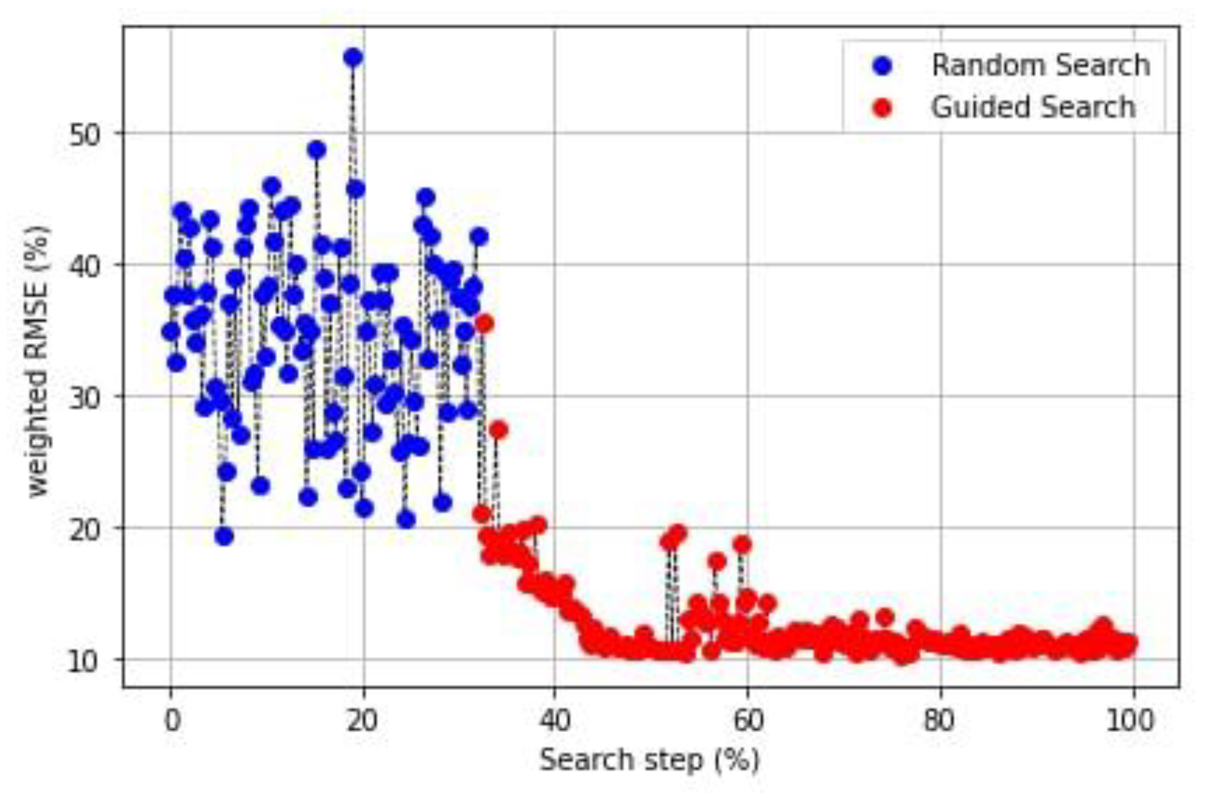
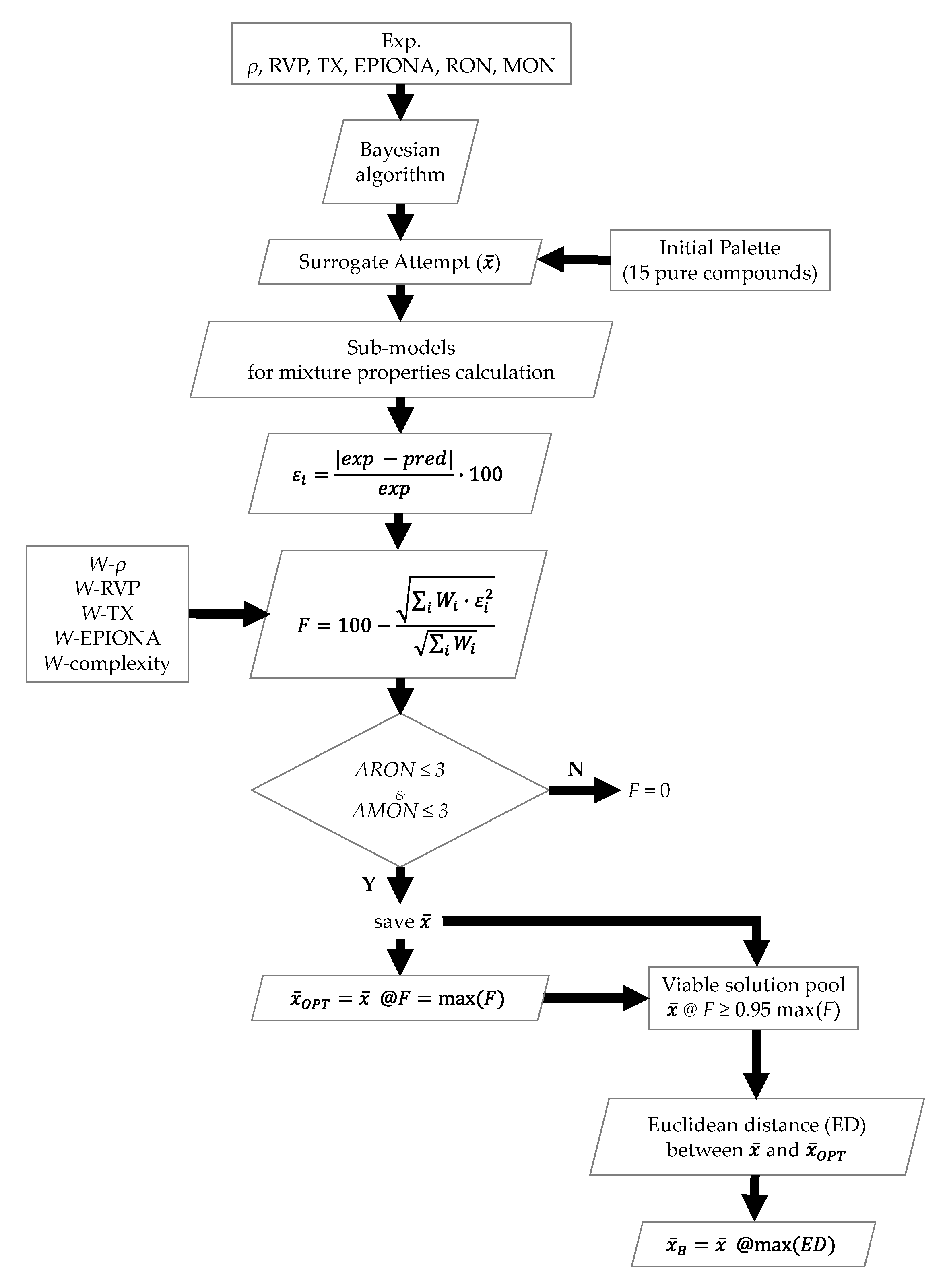
2.3. Surrogate Optimization Strategy

Considering the large number of independent variables (equal to the size of the chosen palette) and the non-linearity of some of the functions needed to reconstruct the target values, the optimization process cannot be addressed by a standard root-finding algorithm. Thus, it needs to be performed with a more complex workflow. State of the art optimization approaches have been successfully applied in literature to this aim. However, a customized implementation of the distillation curve model, to predict the distillation curve of a generic mixture, largely increases the amount of computing time required to run a sufficient number of evaluations. To reduce this effect, a Bayesian optimization algorithm has been employed, which takes advantage of a surrogate model to guide the maximum search. The final algorithm is a combination of the Upper Confidence Bound (UCB) exploration strategy and the use of Gaussian Process Priors as ‘surrogate model’ for the target function. Differently from other algorithms, the Bayesian optimization approach relies on a probabilistic surrogate function, that is continuously updated, to prescribe the next point to be evaluated inside the domain. The reason why Gaussian Processes are usually employed in this application is that (in their classical form) they interpolate precisely the observations on which they were trained. Furthermore, they are a probabilistic algorithm that can simultaneously predict new values and their confidence intervals. Therefore, Gaussian Processes (GP) are suitable in combination with the upper confidence bound acquisition strategy, whose complete acquisition function α is defined in Equation (13), in which X is the evaluation point, K is a tuning hyperparameter indicating the level of ‘thrust’ that is given to the Gaussian Process prediction, μ and σ are the model predicted mean and standard deviation, respectively.

$${\alpha }_{GP-UCB}\left(X, K\right)=\mu \left(X\right)+K·\sigma \left(X\right)$$

(13)

The complete algorithm, inspired by [27], can be resumed as follow: (i) a number of base combinations is initially evaluated, and the objective function is calculated for them; (ii) the Gaussian Process Priors are initially fit to those available data points; (iii) the objective function is evaluated in the point X_MAX that optimizes the acquisition function over the pre-trained Gaussian Process model; (iv) if successive iterations are expected, the Gaussian Process model is updated with the newly evaluated point, else the point X_MAX is returned.

The multi-objective function that the algorithm needs to maximize is defined in Equation (14), where for each i-th target property ε is the percentage absolute relative error between the predicted and the experimental value of the property and W is the weight assigned to the property. In this way, the optimized mixture is placed on a weighted pareto frontier with the minimum Euclidean distance from the optimal composition. The algorithm was implemented with the Bayesian-Optimization open source constrained global optimization tool for Python.

$$\mathrm{F}=100-\frac{\sqrt{{{\displaystyle \sum }}_{\mathrm{i}}{\mathrm{W}}_{\mathrm{i}}·{\mathsf{\epsilon }}_{\mathrm{i}}^2}}{\sqrt{{{\displaystyle \sum }}_{\mathrm{i}}{\mathrm{W}}_{\mathrm{i}}}}$$

(14)

The fuel properties that are taken into account by the objective function, here called primary constraints, are liquid density, RVP, distillation temperatures from T10 to T90 with steps of 10%vol, volumetric chemical macro-composition (EPIONA). In order to limit the number of components, a further primary constraint called ‘complexity’ was added and weighted in the objective function as ${\epsilon }_{complexity}=N/P$, where N is the number of components of the surrogate attempt and P is the size of the initial palette, i.e., 15. As mentioned, RON and MON values are not included in the right-hand-side sum of Equation (14). Instead, they are used as light (secondary) in the following solution screening strategy: (i) an acceptability range of experimental ON ± 3 is defined as threshold; (ii) after each surrogate attempt ($\overline{x}=x_i$, i = 1,…,15), RON and MON values are calculated for the surrogate as in Section 2.2.5; (iii) if the predicted values exceed the acceptability threshold, the objective function F is set at zero, whatever is the value achieved for that point. Once the algorithm has accomplished the optimization task, the screening of the viable solutions (F > 0) is performed, and the surrogate associated with the maximum F value is considered as the optimum (${\overline{x}}_{OPT}=x_{i,OPT}$, i = 1,…,15).

In the surrogate formulation step, the exploration range for the presence of each component is 0–80%vol. Once the surrogate is defined, the components that are present in volume fraction below 4% are automatically excluded and the other components are renormalized according to the reduced composition. It is underlined that for non-oxygenate blends, the possibility to choose ethanol in the surrogate formulation is directly denied by the user i.e., the presence of ethanol is limited at 0%vol. For purely hydrocarbon target blends this is necessary in order to avoid ethanol-blending solutions that could have been promoted by the need to match the RON and MON values.

After internal convergence evaluations, the number of base combinations has been set to 50 to generate a sufficiently accurate model for initializing the search, whilst the maximum number of iterative optimization steps is set to 200. The value of the tuning hyperparameter K has been set to 0.5, with a decay term the more evaluations are performed. The optimized hyperparameters and setting of the machine learning model are listed in

Table 4. List of the optimized hyperparameters of the Bayesian algorithm and user setting parameters.

Parameters	Optimized Set
GP regressor kernel	Matérn
Target variables	normalized
ν	5/2
α	1 × 10−6
K	0.5
Num. initial evaluations	50
Num. maximum optimization iteration	200
W-ρ	1.0
W-RVP	2.5
W-TX	2.0
W-EPIONA	1.5
W-complexity	0.5

in which ν is the smoothness controlling parameter of the function, α is the variance of the additional white noise on the training data.

A general example of the searching process performed by the implemented algorithm is shown in Figure 4, where blue markers and red markers represent exploration and the following exploitation steps, respectively. In Figure 4 it is visible that the Root Mean Squared Error (RSME) approaches an asymptotic minimum value after around a half of the complete searching. In the second half the final solution is refined. The red peaks that are visible in the latter are due to sporadic attempts of further exploration during the refinement that are correlated to the value of the degree of thrust (K).

2.4. Analysis of the Surrogate Unicity

An important point of this work is the evaluation of the ‘unicity’ of the winner surrogate with respect to other minor viable composition solutions which show a different distribution of the accuracy over the properties of interest. Given the optimum surrogate, a further surrogate of the same solution set is selected for comparison as follow: (i) once the optimized surrogate (maximum value of F) has been identified, the solutions comprised in the 5% bound of the maximum F value are considered equally acceptable (F ≥ 0.95 max(F)); (ii) for the solutions that fall in the condition (i), an Euclidean distance from the optimum based on the light constraints (RON, MON) is computed, then the most distant point, here called bound surrogate, is selected for the comparison with the optimum surrogate (${\overline{x}}_B=x_{i,B}$, i = 1,…,15). A schematic view of the workflow is reported in Figure A1.

3. Results

The implemented algorithm has been applied to the formulation of the surrogates for four real gasolines fully experimentally characterized from literature [28,29]. From [28], two Co-Optima gasoline fuels, namely Co-Optima Aromatic and Co-Optima Cycloalkane, have been selected. From [29], the EU6 compliant gasolines Fuel-15 (hydrocarbon blend with properties in line with the current commercial RON95 gasoline) and Fuel-11 (E10 gasoline-ethanol blend) are selected among the available fuels according to Author’s defined criteria i.e., ethanol-blending ≤ E10; RON ≥ 95, olefins volume content ≤ 10%. The main properties of the validation gasolines collected from [28,29] are resumed in

Table A1. Main available useful properties of the validation gasolines, collected from literature.

Properties	A [28]	B [28]	C [29]	D [29]
RON	98.0	98.1	97.8	95
MON	87.1	87.8	85.6	84.9
Density @15 °C (kg/m3)	755.5	757.2	759.6	742.8
RVP (psi)	8.00	7.17	9.93	10.23
T10 (°C)	55.7	59.4	51.4	46.4
T20 (°C)	62.4	72.2	58.7	54.7
T30 (°C)	68.9	84.6	64.5	63.7
T40 (°C)	76.6	96.8	69.2	74.6
T50 (°C)	87.4	108.1	87.4	87.6
T60 (°C)	101.7	116.4	110.6	102.3
T70 (°C)	113.8	124.0	121.9	117.2
T80 (°C)	122.7	136.3	132.2	130.0
T90 (°C)	142.7	157.9	148.1	148.6
C (%wt)	87.08	87.22	83.68	86.88
H (%wt)	13.24	13.12	12.61	12.79
O (%wt)	0	0	3.7	0
Ethanol (%vol.)	0	0	8.54	0
n-Paraffins (%vol.)	6.9	6.7	15.66	17.81
i-Paraffins (%vol.)	28.7	33.9	20.36	30.02
Olefins (%vol.)	1.5	4.1	7.67	7.58
Naphthenes (%vol.)	24	7.9	7.94	7.24
Aromatics (%vol.)	38.4	45.8	38.62	36.11

. It is underlined that the EPIONA of Fuel-11 and Fuel-15 are calculated by the present Authors based on the Detailed Hydrocarbon Analysis (DHA) available in [29]. For the sake of simplicity, in the followings Co-Optima Aromatic, Co-Optima Cycloalkane, Fuel-11, Fuel-15 will be named A, B, C, D, respectively.

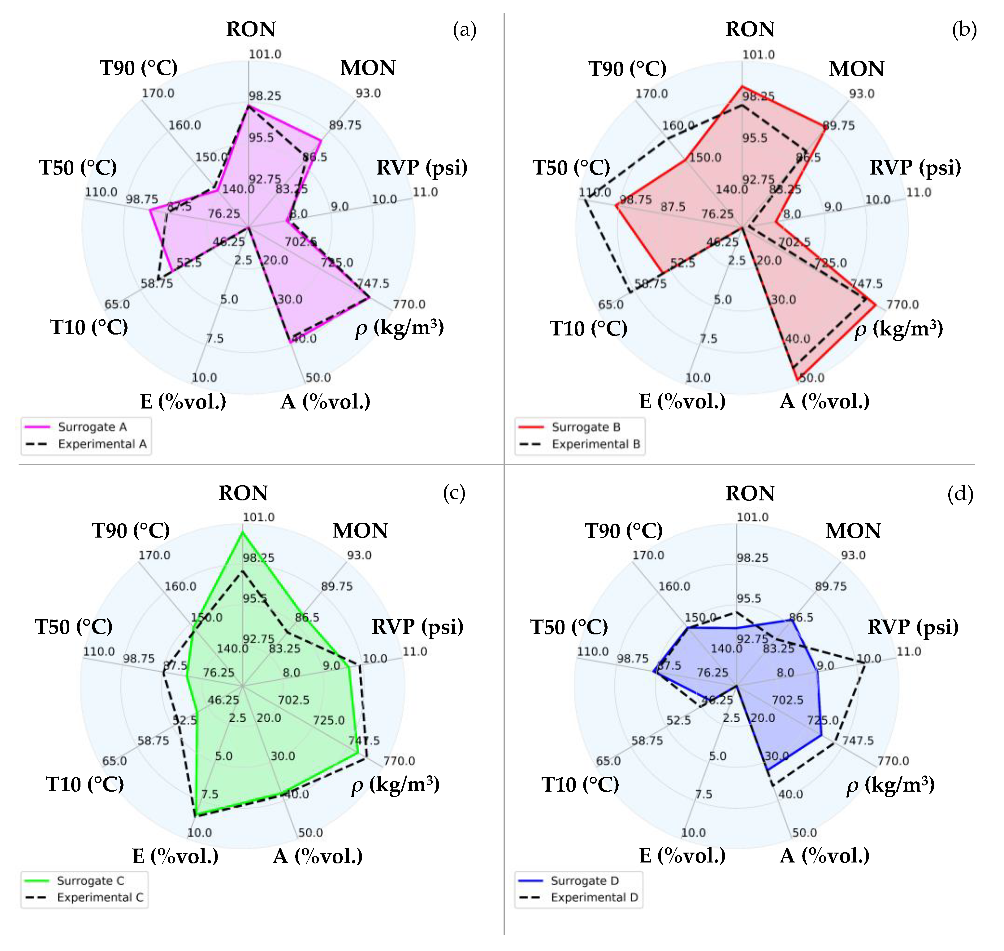
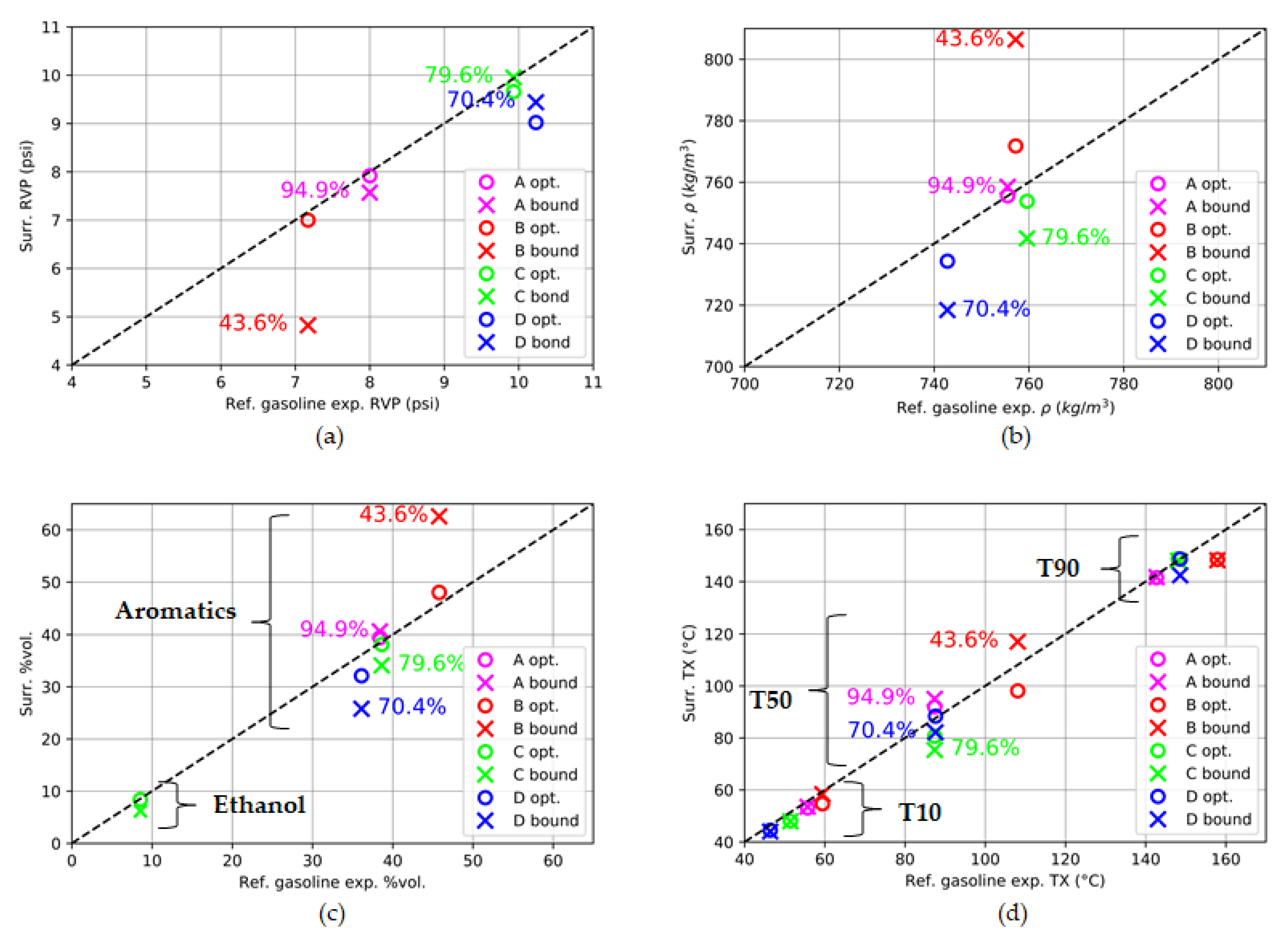
3.1. Optima Surrogates Results

Figure 5 shows both the chemical classes, represented by colors, and the constituting compounds, represented by patterns, of the optima surrogates of the four validation gasolines. Furthermore, the experimental EPIONA composition (empty bars) is also placed at the left of the corresponding surrogate bar. Since surrogates may comprise different compounds that belong to the same chemical class, thus, they would be filled with the same color, a unique pattern is assigned to each compound of a certain chemical class in order to distinguish the stacks of the same chemical class.

It can be observed that the surrogates of A and B gasolines lack of olefins. Since A and B real gasolines are poor in olefins (1.57%vol and 4.54%vol, respectively) the algorithm automatically removes the olefins available in the palette since their target presence is below the minimum threshold (4%vol). The optima surrogates of C and D gasolines are characterized by olefins over-estimation, also missing n-paraffins are observed in the surrogate of C gasoline. Those differences are due to the mutual compensation of RVP and volatility, whose match is searched with greater importance (Table 4). In Figure 5, for each couple of experimental-surrogate bars, an overall nice agreement is visible, in particular for i-paraffins, aromatics and ethanol. Despite the match of each chemical class is pursued with the same weight value, in the results analysis more importance is given to the capture of ethanol, i-paraffins and aromatics composition. This particular focus is due to the key role played by those chemical classes in determining fundamental features of the gasoline evaporation i.e., flattening of the distillation temperature profile in a significant distilled volume range due to oxygenates, average evaporative behavior mainly driven by i-paraffins, delayed evaporation with formation of rich pockets of mixture due to the presence of aromatics. With regards to the species comprised in optima surrogates, in Figure 5 it is visible that heptane and decane are not included in any surrogate formulation due to their non-positive contribution to RON and MON values. The components that are in common between the four optima surrogates are i-pentane, toluene and 1-2-4-trimethylbenzene. It is highlighted that the representation of aromatics required the most various composition. The detailed composition of the optima surrogates is released in

Table A2. Composition of optima surrogates for the four validation gasolines.

Compound (%mol.)	A	B	C	D
Ethanol	0	0	15.44	0
n-Pentane	8.61	0	0	14.31
n-Hexane	0	7.34	0	0
n-Heptane	0	0	0	0
n-Decane	0	0	0	0
i-Pentane	17.06	18.12	18.31	12.06
i-Octane	12.52	6.71	0	10.58
1-Pentene	0	0	13.98	14.39
1-Hexene	0	0	10.14	9.58
Cyclopentane	18.70	16.61	8.83	0
Cyclohexane	9.47	9.15	0	7.21
Toluene	11.51	22.96	7.04	6.59
m-Xylene	6.55	0	0	16.15
Ethylbenzene	8.86	8.37	17.80	0
1-2-4-Trimethylbenzene	6.72	10.74	8.46	9.13
Components	9	8	8	9

.

In Figure 6a, it can be seen that the shape of the distillation curve of the optima surrogates is in solid agreement with experiments along the whole distillation axis. Surrogates of A, C, D gasolines achieve a greater match while a general under-estimation is noticed for the surrogate of B gasoline. Figure 6b shows the temperature difference between the predicted distillation temperature of the surrogate and the experimental value associated to the real gasoline. Dashed lines are placed at ±7 °C, which are here considered as acceptable temperature differences in the validation.

Surrogates of A and D gasolines show temperature differences with experiments below 5 °C along the whole distillation axis. The surrogate of C gasoline as well is is characterized by very low temperature differences even though a predicting performance degradation is shown in the interval T50-T60, where border temperature differences are present. It must be underlined that experimental works in literature [30] have shown that the addition of oxygenates in light-duty gasolines particularly affects the range 30–60%vol. Therefore, it is worth mentioning that an overall accurate prediction (differences below 5 °C) is achieved in this range for the E10 surrogate (C). Thus, a good performance of the algorithm in predicting the evaporation of oxygenates can be expected. The steep increase of the temperature difference in the T50-T60 interval is caused by a performance degradation of the surrogate’s EPIONA composition at the ‘interface’ between the evaporation of the residual ethanol and the first vapor of the next evaporating components. Border difference temperature values can be seen for the surrogate of B gasoline in particular around T50 and T90. This performance decrease is correlated to the high aromatic content of gasoline B (46%vol) with respect to that of A, C, D gasolines (30–35%vol). It is assumed that including more aromatic species in the palette could help to reduce those differences. However, it must be underlined that the aromatics content in nowadays commercial gasolines is limited at maximum values around those reported for A, C, D.

The radar charts in Figure 7 report the comparison between real gasolines and the optima surrogates in terms of light constraints (RON, MON), three key distillation temperatures i.e., T10, T50, T90, two key components from EPIONA i.e., ethanol and aromatics, density, RVP. A general solid agreement can be seen for the surrogates of A (Figure 7a) and C (Figure 7c) gasolines. The properties of gasoline D as well are in a good shape with experimental measures despite the relative error around 10% in predicting the RVP (Figure 7d).

Considering the radar charts in Figure 7a,c,d it is worth mentioning that the bond between chemical (ethanol, aromatics composition) and physical (density, RVP, key distillation temperatures) properties is well captured, furthermore RON and MON values are reasonably reproduced. To the best knowledge of the Authors the current literature lacks of methodologies performing the simultaneous accurate prediction of high-octane gasolines properties such as composition and evaporation features. Thus, the proven capability of the present algorithm to perform this task is worthwhile, in particular for gasolines whose properties are in line with nowadays RON95 (D) and RON98 (A, C) gasolines. As reported for the distillation validation, the surrogate of B gasoline suffers from a general loss of prediction performance as visible in Figure 7b (MON, RVP, T10, T50, T90), confirming the sensitivity of the model to the aromatics content.

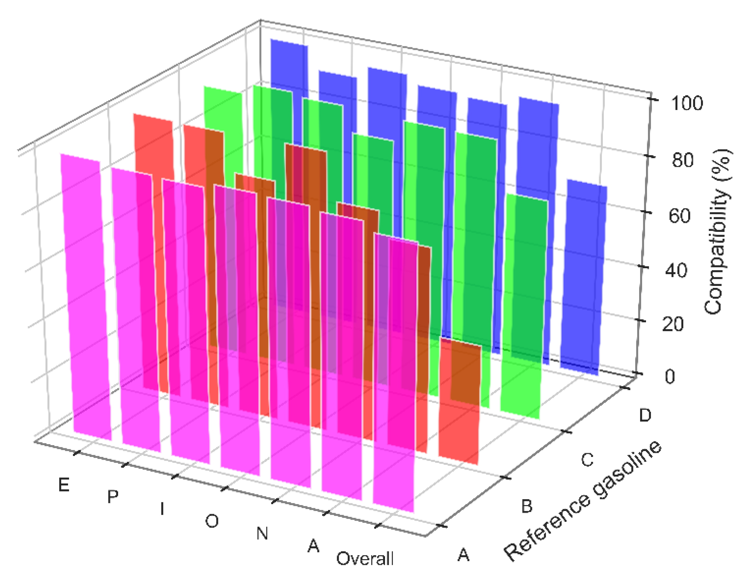
3.2. Composition Unicity

In this section, the results of the ‘winner’ surrogate are compared with the results achieved by the most distant surrogate comprised in the subset of acceptable solutions in the same pool (objective function F ≥ 0.95 max(F)), which will be called bound surrogate. The comparison is performed in order to discuss the ‘unicity’ of the surrogate composition that is assessed by means of the parameter called compatibility, which is defined as in Equation (15), where P is the number of components in the initial palette, x_i,OPT and x_i,B represent the volume fractions of the i-th compound in the optimum surrogate and in the bound surrogate, respectively. Figure 8 reports the results of both the overall and the class-by-class compatibility. It is underlined that the optimum surrogate and the bound surrogate for A, B, D gasolines are fully compatible in ethanol a-priori since the presence of ethanol in those surrogates was constrained at zero by the user, being the real A, B, D gasolines lacking in oxygenates (Table A1).

$$\mathrm{compatibility}=100-{{\displaystyle \sum }}_{\mathrm{i}=1}^{\mathrm{P}}\left({\mathrm{x}}_{\mathrm{i},\mathrm{OPT}}-{\mathrm{x}}_{\mathrm{i},\mathrm{B}}\right)·100$$

(15)

As visible in Figure 8, an almost full compatibility is detected for the two most different surrogates of gasolines A (magenta, 95%) and C (green, 80%), confirming the solidity of those surrogates. Therefore, it is observed that the need of accuracy in predicting the evaporative features of those gasolines converges towards an about unique possible composition. The high compatibility in ethanol (96%) achieved by the two most different surrogate solutions of C gasoline is a further sign that the algorithm clearly identifies the role of the ethanol addition. A lower overall compatibility is detected between the two surrogates of D gasoline (blue, 70.5%) due to slight differences in the compatibility of each single chemical class and a significant n-paraffinic incompatibility caused by the replacement of n-pentane with n-hexane (Table A2). On the other hand, the composition variability between the two surrogates representing B gasoline (red) is large, indeed the overall compatibility of the bound surrogate is around 43%. The latter is mainly due to the low aromatic compatibility, which is around 70%. As reported in Table A1, the properties of B gasoline and A gasoline are similar except for the aromatics content (45%vol against 38%vol), which in its turn affects the distillation temperature differences. The compatibility analysis suggests that the ‘unicity’ of the surrogate formulation as well is very sensitive to the presence of aromatics.

The sensitivity of the target properties to the different levels of compatibility is shown in the following parity plot figures (Figure 9), where the value of compatibility is reported next to the respective bound surrogate marker.

As expectable, the lower is the level of compatibility, the larger is the bound-optimum difference in predicting the properties. However, different sensitivities to the variability of the composition are experienced by different properties. It is visible that regardless to the level of compatibility, an increasing composition sensitivity is detected for the RVP (Figure 9a), distillation temperatures (Figure 9d), composition (Figure 9c), density (Figure 9b), respectively. Considering Table 4, it is clear that for different surrogates of the same solution pool that reasonably accomplish the accuracy target, the higher is the importance (weight value) given to the target property, the lower is its sensitivity to the composition variability of the surrogate. It must be noticed that a high level of compatibility is a sign of robustness and reliability of the surrogate solution. From Figure 9 it is clear that the compatibility recorded in a pool of surrogate solutions is correlated to the prediction performance. Indeed, the higher levels of compatibility (green, 80% and magenta 95%) provide an improved prediction performance over the whole set of target properties, whilst lower levels of compatibility may result in good performance on some target properties and significant mismatch on others. As a result, one can assume that the high degree of accuracy equally distributed over the presented target properties relies on the ‘unicity’ of the surrogate composition (high compatibility). Whether the ‘unicity’ of the surrogate composition is always achievable remains an open quest that needs further validation and strongly depends on the size and the variety of the base palette, the maximum number of components allowed in the surrogate and the capability of the searching algorithm to target the proper space of solutions in affordable computation times.

4. Discussion

This work deals with the implementation of a machine-learning based methodology to identify the proper surrogate for nowadays and future gasolines to provide three-dimensional CFD engine simulations under fuel stratification operations. Different in-house developed sub-models and a customized searching algorithm have been developed. A palette of 15 different pure compounds is provided to the searching algorithm. A Bayesian optimization strategy is implemented to evaluate different compositions with the aim to achieve the optimum surrogate according to a merit function defined to pursue the minimum Euclidean distance between experimental and surrogate targets namely, density, Reid vapor pressure, chemical macro-composition, distillation properties, number of components. RON and MON of the surrogate are constrained at a maximum difference of 3 units with respect to experimental values. The methodology is applied to identify the optima surrogates of four different gasolines fully experimentally characterized in literature. The implemented algorithm has proven to be capable to perform a fine prediction of the target properties of two hydrocarbon-blend gasolines and one ethanol-gasoline blend, whose characteristics are in line with the nowadays requirements for commercial gasolines i.e., RON 95–98, olefins < 10%vol and aromatics < 35%vol. Performance losses are detected in predicting the RVP and the distillation curve of the fourth gasoline, which differs from the others by a higher aromatics content (45%vol). Therefore, it is found that the formulation of surrogates aimed to mimic the evaporative features of real gasolines are very sensitive to the presence of aromatics. The possibility to achieve a ‘unique’ surrogate composition to provide CFD codes is also discussed by comparing optima results with the most different surrogate characterized by almost the same value of the merit function (i.e., same overall accuracy). The comparison is performed by means of a synthetic index introduced by the present Authors, namely the compatibility, which reports the degree of likeness between the optimum solution and the most different acceptable solution. For the three gasolines characterized by the standard presence of aromatics, high levels of compatibility (70–95%) are observed, meaning that the composition capable to accomplish the emulation of the evaporative features properly is about unique. Considering the results for the gasoline characterized by the high presence of aromatics, a significant sensitivity of the compatibility (43%) to the aromatics composition is revealed. A further worth mentioning result is that the compatibility analysis has shown that the higher is the level of compatibility between the two most different surrogates of the solution pool, the higher is the level of accuracy in predicting each target property. Therefore, compatibility has proven to be an index of the reliability of the identified surrogate. As a result, four optima surrogates comprising 8–9 components are achieved based on the target accuracy. It is underlined that the present Authors have tested those surrogates in 3D-CFD simulations with multi-component spray injection and evaporation. Despite the fact that the number of components is slightly greater than that of common practice surrogates (6–7 components), the overall computation time is not affected significantly. Therefore, the surrogates identified in the present work can be used for three-dimensional CFD calculations with no concerns on the time spent.

References

1. Nakai, E.; Goto, T.; Ezumi, K.; Tsumura, Y.; Endou, K.; Kanda, Y.; Urushihara, T.; Sueoka, M.; Hitomi, M. Mazda Skyactiv-X 2.0L gasoline engine. In Proceedings of the 28th Aachen Colloquim Automobile and Engine Technology Aachen, Germany, 7–9 October 2019; Eckstein, L., Pischinger, S., Heetkamp, M., Müller, J., Eds.; Institute for Automotive Engineering, RWTH: Aachen, Germany, 2019. [Google Scholar]
2. Dempsey, A.B.; Curran, S.; Wagner, R. A perspective on the range of gasoline compression ignition combustion strategies for high engine efficiency and low NOx and soot emissions: Effects of in-cylinder fuel stratification. Int. J. Engine Res. 2016, 17, 897–917. [Google Scholar] [CrossRef]
3. Sjoberg, M.; Dec, J.E. Smoothing HCCI Heat-Release Rates Using Partial Fuel Stratification with Two-Stage Ignition Fuels. SAE Tech. Pap. Ser. 2006, 10, 4271. [Google Scholar] [CrossRef]
4. Priyadarshini, P.; Sofianopoulos, A.; Mamalis, S.; Lawler, B.; Lopez-Pintor, D.; Dec, J. Understanding partial fuel stratification for low temperature gasoline combustion using large eddy simulations. Int. J. Engine Res. 2021, 22, 1872–1887. [Google Scholar] [CrossRef]
5. Zhou, L.; Hua, J.; Wei, H.; Dong, K.; Feng, D.; Shu, G. Knock characteristics and combustion regime diagrams of multiple combustion modes based on experimental investigations. Appl. Energy 2018, 229, 31–41. [Google Scholar] [CrossRef]
6. Hu, Z.; Zhang, J.; Sjöberg, M.; Zeng, W. The use of partial fuel stratification to enable stable ultra-lean deflagration-based Spark-Ignition engine operation with controlled end-gas autoignition of gasoline and E85. Int. J. Engine Res. 2020, 21, 1678–1695. [Google Scholar] [CrossRef]
7. Mehl, M.; Chen, J.-Y.; Pitz, W.J.; Sarathy, S.M.; Westbrook, C.K. An Approach for Formulating Surrogates for Gasoline with Application toward a Reduced Surrogate Mechanism for CFD Engine Modeling. Energy Fuels 2011, 25, 5215–5223. [Google Scholar] [CrossRef]
8. Abianeh, O.S.; Oehlschlaeger, M.A.; Sung, C.-J. A surrogate mixture and kinetic mechanism for emulating the evaporation and autoignition characteristics of gasoline fuel. Combust. Flame 2015, 162, 3773–3784. [Google Scholar] [CrossRef] [Green Version]
9. Ahmed, A.; Goteng, G.; Shankar, V.S.B.; Al-Qurashi, K.; Roberts, W.L.; Sarathy, S.M. A computational methodology for formulating gasoline surrogate fuels with accurate physical and chemical kinetic properties. Fuel 2015, 143, 290–300. [Google Scholar] [CrossRef]
10. Daly, S.R.; Niemeyer, K.E.; Cannella, W.J.; Hagen, C.L. FACE Gasoline Surrogates Formulated by an Enhanced Multivariate Optimization Framework. Energy Fuels 2018, 32, 7916–7932. [Google Scholar] [CrossRef]
11. Grubinger, T.; Lenk, G.; Schubert, N.; Wallek, T. Surrogate generation and evaluation of gasolines. Fuel 2021, 283, 118642. [Google Scholar] [CrossRef]
12. Cheng, S.; Saggese, C.; Kang, D.; Goldsborough, S.S.; Wagnon, S.W.; Kukkadapu, G.; Zhang, K.; Mehl, M.; Pitz, W.J. Autoignition and preliminary heat release of gasoline surrogates and their blends with ethanol at engine-relevant conditions: Experiments and comprehensive kinetic modeling. Combust. Flame 2021, 228, 57–77. [Google Scholar] [CrossRef]
13. Pati, A.; Gierth, S.; Haspel, P.; Hasse, C.; Munier, J. Strategies to Define Surrogate Fuels for the Description of the Multicomponent Evaporation Behavior of Hydrocarbon Fuels. SAE Tech. Pap. Ser. 2018, 10, 4271. [Google Scholar] [CrossRef]
14. Muelas, Á.; Aranda, D.; Ballester, J. Alternative Method for the Formulation of Surrogate Liquid Fuels Based on Evaporative and Sooting Behaviors. Energy Fuels 2019, 33, 5719–5731. [Google Scholar] [CrossRef]
15. Zhu, L.; Gao, Z.; Cheng, X.; Ren, F.; Huang, Z. An assessment of surrogate fuel using Bayesian multiple kernel learning model in sight of sooting tendency. Front. Energy 2021, 27, 1–15. [Google Scholar] [CrossRef]
16. Green, D.W.; Southard, M.Z. Perry’s Chemical Engineers’ Handbook, 9th ed.; McGraw Hill: New York, NY, USA, 2019; pp. 5–93. [Google Scholar]
17. McCormick, R.; Fioroni, G.; Fouts, L.; Christensen, E.; Yanowitz, J.; Polikarpov, E.; Albrecht, K.; Gaspar, D.; Gladden, J.; George, A. Selection Criteria and Screening of Potential Biomass-Derived Streams as Fuel Blendstocks for Advanced Spark-Ignition Engines. SAE Int. J. Fuels Lubr. 2017, 10, 442–460. [Google Scholar] [CrossRef]
18. Meyers, R.A. Handbook of Petroleum Refining Processes, 3rd ed.; McGraw Hill: New York, NY, USA, 2004; pp. 308–383. [Google Scholar]
19. Slavinskaya, N.A.; Zizin, A.; Aigner, M. On Model Design of a Surrogate Fuel Formulation. J. Eng. Gas Turbines Power 2010, 132, 111501. [Google Scholar] [CrossRef]
20. Abianeh, O.S.; Chen, C.P.; Cerro, R.L. Batch Distillation: The Forward and Inverse Problems. Ind. Eng. Chem. Res. 2012, 51, 12435–12448. [Google Scholar] [CrossRef]
21. Soave, G. Equilibrium constants from a modified Redlich-Kwong equation of state. Chem. Eng. Sci. 1972, 27, 1197–1203. [Google Scholar] [CrossRef]
22. Wilson, G. A modified Redlich-Kwong equation of state applicable to general physical data calculations. In Proceedings of the 65th AIChE National Meeting, Cleveland, OH, USA, 4–7 May 1968. [Google Scholar]
23. Bruno, T.J.; Smith, B.L. Evaluation of the Physicochemical Authenticity of Aviation Kerosene Surrogate Mixtures. Part 1: Analysis of Volatility with the Advanced Distillation Curve. Energy Fuels 2010, 24, 4266–4276. [Google Scholar] [CrossRef]
24. Ferris, A.M.; Rothamer, D. Methodology for the experimental measurement of vapor–liquid equilibrium distillation curves using a modified ASTM D86 setup. Fuel 2016, 182, 467–479. [Google Scholar] [CrossRef] [Green Version]
25. Greenfield, M.L.; Lavoie, G.A.; Smith, C.S.; Curtis, E.W. Macroscopic Model of the D86 Fuel Volatility Procedure. SAE Tech. Pap. Ser. 1998, 10, 4271. [Google Scholar] [CrossRef]
26. Anderson, J.E.; Leone, T.G.; Shelby, M.H.; Wallington, T.J.; Bizub, J.J.; Foster, M.; Lynskey, M.G.; Polovina, D. Octane Numbers of Ethanol-Gasoline Blends: Measurements and Novel Estimation Method from Molar Composition. SAE Tech. Pap. Ser. 2012, 10, 17. [Google Scholar]
27. Brochu, E.; Cora, V.; Freitas, N. A Tutorial on Bayesian Optimization of Expensive Cost Functions, with Application to Active User Modeling and Hierarchical Reinforcement Learning. arXiv 2010, arXiv:1012.2599v1. [Google Scholar]
28. Chuahy, F.D.; Powell, T.; Curran, S.J.; Szybist, J.P. Impact of fuel chemical function characteristics on spark assisted and kinetically controlled compression ignition performance focused on multi-mode operation. Fuel 2021, 299, 120844. [Google Scholar] [CrossRef]
29. EPAct/V2/E-89: Assessing the Effect of Five Gasoline Properties on Exhaust Emissions from Light-Duty Vehicles Certified to Tier 2 Standards. Available online: www.epa.gov/moves/epactv2e-89-tier-2-gasoline-fuel-effects-study (accessed on 15 June 2021).
30. Andersen, V.F.; Anderson, J.; Wallington, T.J.; Mueller, S.A.; Nielsen, O.J. Distillation Curves for Alcohol−Gasoline Blends. Energy Fuels 2010, 24, 2683–2691. [Google Scholar] [CrossRef]
Figure 1. Sketch of the experimental distillation process. Gray squares represent the areas of interest of the modeling steps.
Energies 14 04623 g001
Figure 2. Experimental (markers) and predicted (dashed lines) distillation curves (kettle temperatures) for six validation mixtures of known composition from literature.
Energies 14 04623 g002
Figure 3. Absolute relative error in predicting the distillation kettle temperature for six validation mixture (marker-lines) from literature and their mean absolute relative error (solid line).
Energies 14 04623 g003
Figure 4. RMSE profile in the two phases (exploration (blue) and exploitation (red)) of the searching performed by the implemented Bayesian algorithm.
Energies 14 04623 g004
Figure 5. Volumetric composition of the optimum surrogate (filled bars) for the four validation gasolines: the filling color represents the EPIONA composition; the filling pattern represents the constituting pure compounds. Experimental EPIONA volumetric composition (empty bars) is also provided.
Energies 14 04623 g005
Figure 6. Comparison of the distillation curve of the experimental gasoline (markers) and of the optima surrogate (solid line) for the four validation surrogates A, B, C, D (a). The distillation temperature difference between surrogate and experimental values are also shown (b), dashed black lines are placed at ± 7 °C as acceptability interval.
Energies 14 04623 g006
Figure 7. Comparison between different properties (RON, MON, RVP, liquid density (ρ), aromatics volume, ethanol volume, T10, T50, T90) of the optima surrogates (filled polygon) and of the associated experimental gasoline (dashed-line empty polygon). The comparison is shown for the four validation gasolines A (a), B (b), C (c), D (d).
Energies 14 04623 g007
Figure 8. EPIONA class-by-class and overall composition compatibility of optima and bound surrogates of the four validation gasolines (A, B, C, D). The compatibility is calculated as the difference between the volume fraction of each constituting compound.
Energies 14 04623 g008
Figure 9. Parity plot of RVP (a), density (b), Ethanol and Aromatics composition (c), key distillation temperatures (d) for the optimum surrogate (circle) and the bound surrogate (cross) for the four validation gasolines A, B, C, D. Values of the overall compatibility between optimum and bound surrogates composition are also reported next to the markers.
Energies 14 04623 g009