
Dynamic Uncertain Causality Graph Applied to the Intelligent Evaluation of a Shale-Gas Sweet Spot


1
Department of Computer Science and Technology, Tsinghua University, Beijing 100084, China
2
School of Emergency Technology and Management, North China Institute of Science & Technology, Langfang 065201, China
*
Author to whom correspondence should be addressed.
Energies 2021, 14(17), 5228; https://0-doi-org.brum.beds.ac.uk/10.3390/en14175228
Submission received: 29 July 2021
/
Revised: 21 August 2021
/
Accepted: 22 August 2021
/
Published: 24 August 2021
(This article belongs to the Collection Artificial Intelligence and Smart Energy)
Abstract
:Shale-gas sweet-spot evaluation as a critical part of shale-gas exploration and development has always been the focus of experts and scholars in the unconventional oil and gas field. After comprehensively considering geological, engineering, and economic factors affecting the evaluation of shale-gas sweet spots, a dynamic uncertainty causality graph (DUCG) is applied for the first time to shale-gas sweet-spot evaluation. A graphical modeling scheme is presented to reduce the difficulty in model construction. The evaluation model is based on expert knowledge and does not depend on data. Through rigorous and efficient reasoning, it guarantees exact and efficient diagnostic reasoning in the case of incomplete information. Multiple conditional events and weighted graphs are proposed for specific problems in shale-gas sweet-spot evaluation, which is an extension of the DUCG that defines only one conditional event for different weighted function events and relies only on the experience of a single expert. These solutions make the reasoning process and results more objective, credible, and interpretable. The model is verified with both complete data and incomplete data. The results show that compared with other methods, this methodology achieves encouraging diagnostic accuracy and effectiveness. This study provides a promising auxiliary tool for shale-gas sweet spot evaluation.
1. Introduction
Shale gas, as an unconventional green energy source in the petroleum industry, has received increasing attention since 2005. Owing to the current environmental problems and resource-intensive energy development, effectively developing China’s shale-gas resources on a large scale is an urgent task of substantial research value and significance. At present, domestic shale-gas exploration and development is rapidly growing. The main research focus is combining the achievements and experience of experts and scholars; using the evaluation results of different areas to divide them into target areas, favorable areas, and sweet spots to reduce the risks related to shale-gas exploration and development; and obtaining economic benefits from oilfields [1,2,3].
There are many evaluation methods for the exploration and development of various types of oil and gas reservoirs. Wang proposed new equations for characterizing water flooding in the production prediction of ultra-high water-cut reservoirs [4]. Zhang proposed the queued competition algorithm to calculate shale-gas production reserves and established a shale-gas production reserve optimization model [5]. Jiang proposed the sequential fully implicit (SFI) scheme for solving coupled flow and transport problems [6]. Zhou proposed a new method for evaluating favorable shale-gas exploration areas based on multi-linear regression analysis [7]. Chen comprehensively analyzed the features of the Logistic model, the Gompertz model, and the Usher model to establish an optimal combination forecasting model of the water cut of a water flood field [8]. Li proposed several random models based on the analysis of uncertain variables, and the models were optimized to detain the reservoir development index prediction [9]. Zhong proposed that the knowledge mining process based on deep learning may help autonomously obtain an appropriate prediction model of the oilfield development index [10]. Daniel proposed the application of supervised machine learning paradigms in the prediction of petroleum reservoir properties by comparing and analyzing artificial neural network (ANN) and support vector machine (SVM) models [11]. Wang outlined an analytic hierarchy process to optimize the favorable area of tight oil [12]. Shang used the analytic hierarchy process to solve the contradiction of single-parameter classification for traditional low-quality reserves [13]. Guan established an optimization hierarchical structure model of shale-gas exploration area assessment by using the analytical hierarchy process: goal layer, criterion layer, sub-criterion layer, and project layer [14].
Most of the above evaluation methods require a relatively large amount of sample data and accurate data-related information. However, problems, such as lack of data, imprecise information, and the inconsistent experience of experts in the initial stages of exploration and development, have not been properly addressed. In the middle and late stages of exploration and development, even when relatively complete geological information is available, the development benefit is subject to new uncertainties due to the nonhomogeneity of the reservoir structure and the change in economic factors.
Lack of data and imprecise, inconsistent, and incomplete information, combined with multiple-expert knowledge, make it challenging to intuitively and clearly complete the diagnosis of complex systems and realize high scalability and accurate reasoning in the field of oil and gas reservoir sweet-spot evaluation.
In recent years, the knowledge representation and reasoning methods based on the dynamic uncertainty causality graph (DUCG) have made great progress in industrial system fault diagnosis [15,16,17] and the auxiliary diagnosis of diseases [18,19,20,21]. In this study, the DUCG was applied to predict a shale-gas sweet spot for the first time. A causality model of uncertainty evaluation was also established. However, due to the particularity of shale-gas sweet-spot evaluation, the existing DUCG cannot address some specific problems. We extended the existing DUCG and introduced it in detail. The purpose of this study was to inspire rather than replace the thinking of reservoir experts; to guide and inspire their evaluation process in a reasonable, intuitive, and convenient way; and to establish an evaluation method for shale-gas sweet spots that integrates expert knowledge. As an auxiliary tool, the study provides detailed and reliable knowledge, experience, methods, and ideas regarding shale-gas sweet spots and reduces unnecessary geological experiments and numerical simulation.
The structure of this paper is as follows: Section 2 describes the proposed method based on the DUCG, including the uncertain causality representation, the probabilistic reasoning process, and the DUCG extension. Section 3 introduces the construction process of the evaluation model. In Section 4, verification experiments are presented with complete and incomplete data. Section 5 contains the conclusions.
2. Methods
The DUCG uses graphical representation to resolve the causality between uncertain information and probability measurement. The DUCG is a probability graph model that visually represents causality between variables in a clear pattern and uses chaining reasoning algorithms to achieve efficient reasoning.
2.1. Causality Representation
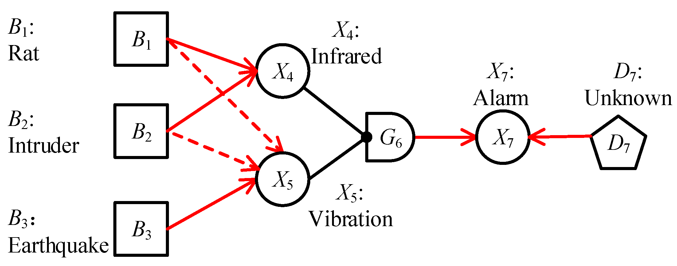
As shown in Figure 1, the DUCG includes a set of variables or events and directed arcs pointing from the cause to the result.
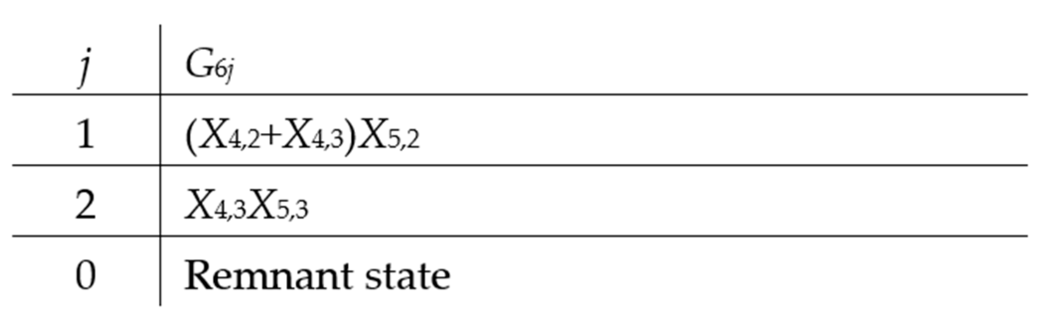
A B-type variable (square-shaped node) represents a root cause event, which is the hypothetical event variable (evaluation result) in the inference calculation. An X-type variable (oval-shaped node) represents a result event variable (evaluation indicators) and can also be used as the cause event of other events. A G-type (logic gate node) variable represents the combinational logic relations between its input and output events, e.g., G6 in Figure 1, with its state expression specified in Figure 2. A D-type variable (pentagon node) represents the default or unspecified cause of an X-type variable. Variable Vi,j represents a parent event of Xn, V∈{B, X, G, D}, n indexes the child variable X, k denotes the variable’s state, i indexes the parent variable V, and j denotes the variable’s state. State j = 0 indicates an uninterested state, and j ≠ 0 indicates an interested state.
The red directed arc represents a weighted functional event, Fnk;ij ≡ (rn;i/rn)Ank;ij describes the causality between a child event Xnk and a parent event Vij, and Ank;ij denotes the independent causality function that Vij does cause Xnk. The weighting factor rn;i represents the intensity of causality between Xn and Vi, where rn;I > 0 and . As a weighting coefficient of An;i, rn;i/rn balances these independent causality functions for all parent events on the same child event.
The dashed directed arc represents a conditional weighted functional event. When the condition Zn;i between a child event Xn and a parent event Vi is met, the dashed arc is converted into a solid arc; otherwise, it is deleted. In the DUCG, the variable identifiers in lowercase letters denote the probability parameters of variables in corresponding uppercase letters, for example, bij = Pr{Bij}, ank;ij = Pr{Ank;ij}.
2.2. Probabilistic Reasoning
In the DUCG, the multivalued causality between each parent–child variable pair can be expressed relatively independently and the causality between variables is expanded by weighted functional events. The child variable Xnk can be expanded into the sum-of-product expression of a series of independent events according to its causality, as shown in Equation (1); the event expansion of the DUCG is shown in Figure 3 [22].
E is the received evidence, and Hkj is the hypothesis event to be solved that is composed of {B, X, A}-type events. The reasoning process for the DUCG is as follows:
- 1.
- Simplification
After evidence E is observed, a large and complex original DUCG can be reduced to a small and simple DUCG according to rules 1–10 [22] and 16 [23].
- 2.
- Decomposition
On the basis of evidence E, by assuming a different initiating event Bi, the DUCG simplified in step 1 can be divided into a set of sub-DUCGs, which can be further simplified according to the rules. Bi is added to the hypothetical space SH.
- 3.
- Event outspread
According to each sub-DUCG, step 1 is repeated to expand all Ej (E = ∏jEj); by combining them with logical operations, the final expression of the E expansion is obtained by combining {B, D, A, r}-type events and parameters. Similarly, HkjE can be expanded to an expression containing only {B, D, A, r} types of events and parameters.
- 4.
- Probabilistic calculation
The parameters of {b, a, r} type are given by domain experts when constructing the DUCG. Hkj denotes possible hypothetical events, and Pr{E} and Pr{HkjE} in each sub-DUCG can be calculated. For the whole simplified DUCG, the probability calculation includes state- and ranking-probability calculations. The formula of the state-probability calculation is as follows:
where hskj is the posterior probability of Hkj; the ranking probability of Hkj is as follows:
Obviously, . All hypothetical events are ranked according to ranking probability. When only one hypothetical event exists, the event is uniquely determined.
The inference calculation of the DUCG is chain- and self-dependent, and the probability of each causal chain only depends on the causal chain itself. Therefore, parameters that are not in the causal chain can be ignored without affecting the correctness of the reasoning. As a result, the DUCG can still complete precise reasoning under conditions of incomplete knowledge representation and missing parameters [22].
2.3. Extension of DUCG
2.3.1. Multiple Conditional Events
The existing DUCG conditional variable has only one conditional event, Zn;i, but each evaluation indicator in the evaluation of oil and gas reservoir sweet spots is in more than one state and the relationship among the evaluation indicators is more complicated. It is difficult to clearly represent the relationship between the parent variable Vi and the child variable Xn with a conditional event Zn;i. This paper introduced multiple conditional events Znk;ij to expand Zn;i. Znk;ij denotes the condition when state j of the parent variable Vi and state k of the child variable Xn satisfy causality. As illustrated in Figure 4, F3;1 is a conditional causality. Without losing generality, suppose there are two states for each variable, states 0 and 1, and the condition is Z3,1;1,1 = X2,0; i.e., only when X2 is in state 0 does F3,1;1,1 exist; otherwise, F3,1;1,1 is eliminated.
2.3.2. Weighted Graph
The concept of a weighted graph was proposed to deal with unknown variables or combine the knowledge of multiple experts. DUCGk denotes the weighted graph generated according to each state k of the unknown variable, and ωi denotes the probability of the weighted graph indexed by i. Because the weighted graphs may have different structures, it was necessary to determine each weighted graph before reasoning and then reason in each weighted graph in a conventional way: (1) simplification, (2) decomposition, (3) event outspread, and (4) probabilistic calculation.
The probability calculation of a weighted graph is expressed differently from Equation (2), as shown in Equation (4).
where E•DUCGi denotes evidence E in DUCGi.
The application of a weighted graph is illustrated in detail in Section 4.2.
3. Evaluation Model Construction
The method of establishing the evaluation model and empirical analysis of shale-gas sweet spots based on the DUCG is summarized as follows:
- 1.
- Variable definition
The definition of variables followed the actual situation of shale-gas exploration and development and selected suitable evaluation indicators on the basis of geological, engineering, and economic factors.
- 2.
- Knowledge representation
To determine causalities between shale-gas sweet spots and each evaluation factor, the evaluation model was constructed by using the statistics, authoritative research results, and domain knowledge related to the oil storage project to determine causality functions’ parameter data.
- 3.
- Probability reasoning
The data of relevant shale-gas examples in the Sichuan basin were selected to reason about the established evaluation model.
- 4.
- Comprehensive comparison
After comparing with the evaluation results of existing evaluation methods, such as hierarchical analysis, the feasibility of evaluation methods proposed in this study was verified.
3.1. Screening Critical Factors for Shale-Gas Exploration and Development
Based on China’s geological structure, experts and scholars often mention the concept of sweet spots and favorable areas in domestic oil field exploration and development. Wang [24] reported that according to the characteristics of China’s shale-gas resources, shale-gas distribution areas are divided into three levels: shale-gas exploration and development target, favorable, and prospecting areas. According to the complexity of the developmental geological conditions, Li [25] established three categories of phases: sea, land and sea transitional, and land phases. According to the characteristics of reservoirs of dense oil, Bao [26] divided dense oil into development-favorable areas I, II, and III. Yang [27] suggested China’s favorable shale-layer evaluation standards, and the evaluation criteria for domestic and foreign dense and shale oil were summarized.
In this study, in the regional evaluation of shale-gas exploration and development, following the experience and achievements of each expert, shale gas was divided into three regions: target areas (level I sweet spots), favorable areas (level II sweet spots), and prospective areas (level III sweet spots). There were three main considerations. First, shale gas cannot solely rely on natural energy but needs more complex development technology, and the investment cost is high. Therefore, it is necessary to ensure that a sweet spot has economic benefits, in addition to existing process technology and production costs. At this time, shale-gas target areas are preferred as the main development areas. Second, with the development of science and technology, some favorable or prospective areas that do not have economic benefits may become new target areas. Therefore, favorable and prospective areas should be determined as soon as possible to provide a basis for shale-gas development planning. Lastly, there are subtle differences in the value range of shale-gas indicators among experts, so it is necessary to establish an expert knowledge system model to effectively combine the geological factors of each basin with the research results of experts and scholars to form geological factors with an expert knowledge background. Combining engineering and economic factors, reasonable uncertainty evaluation methods are selected to build the evaluation models of various reservoir areas [27].
There are three main factors in the evaluation of shale-gas sweet spots: geological, engineering, and economic.
Geological factors in the evaluation of shale-gas sweet spots mainly include organic matter, favorable areas, gas content, and tectonic settings. Organic matter is evaluated in terms of its thickness, total organic carbon, and maturity. The thickness of shale reservoirs is calculated vertically to ensure the scale of shale-gas exploitation; the more the thickness, the higher the sweetness of the area, and the larger the exploitation scale. Organic maturity is key to the formation of shale-gas reservoirs. When the maturity of the organic matter in shale is more than 1.1%, the area is in the range of the gas window. For shale-gas sweet spots, organic matter maturity should be in the range of 1.1% to 2.5%. A favorable area is determined horizontally to calculate the scale of shale-gas exploitation. The favorable area of the target area should be more than 2500 km2. The favorable area and the organic matter thickness are combined to ensure the entire shale-gas sweet-spot content. The gas content of shale-gas reservoirs is the most direct reflection of the economic value of the target area, and its value in the target area should be greater than 4 m3/t. The tectonic background plays a key role in the development of shale-gas reservoirs and creates corresponding requirements for the development technology of shale gas.
Engineering factors in the evaluation of shale-gas sweet spots mainly include the burial depth, the pressure coefficient, the natural cracks, and surface conditions. Shale-gas sweet spots should have a burial depth exactly between 1.5 and 3.5 km. The pressure coefficient also plays a critical role in shale-gas generation. The storage and development stages have a direct impact; thermostatic gas is the product of a high-pressure free state, biogenic gas is the main product of a low-pressure absorption state, and gas content is generally positively related to the pressure coefficient. The degree of the development and pressure coefficient of natural cracks solves the problem of poor reservoir quality to a certain extent, and the surface quality also determines the complexity of the project and affects the evaluation of shale-gas sweet spots.
Economic factors in the evaluation of shale-gas sweet spots mainly include market demand and infrastructure. Market demand is the main economic driving force of shale-gas exploitation. If the evaluation area is already around the pipe network, no more investment is needed to construct the pipe network; if it is far away from the pipe network, costs increase.
The following sections establish the causality relationship between evaluation indicators and a shale-gas sweet spot on the basis of these main factors and use the DUCG to evaluate an area.
3.2. Establishment of the Evaluation Model for Shale-Gas Sweet Spots
3.2.1. Define Variables
The above analysis shows that shale-gas sweet-spot evaluation needs to consider geological, engineering, and economic factors. The current industry standards in the field of petroleum engineering are analyzed and researched in Table 1, and the current industry expert research results are analyzed and researched in Table 2. We selected the latest domestic research results and the experience of experts in the field and the evaluation standard as the evaluation indicators in the evaluation model [14], which is the main basis for constructing the DUCG reasoning model of shale-gas sweet-spot evaluation.
On the basis of industry standards in Table 1 and the results of authoritative experts in Table 2, the main factors were selected to establish an evaluation model, as shown in Figure 5.
In the DUCG, the three types of shale-gas sweet spots are defined as root nodes (B-type variables). As mentioned in Section 3.1, evaluation indicators of geological sweet spots are organic matter (evaluated in terms of thickness, total organic carbon, and maturity), favorable areas, gas content, and tectonic background; evaluation indicators of engineering sweet spots are the burial depth, the pressure coefficient, natural cracks, and surface conditions; and evaluation indicators of economic sweet spots are market demand and infrastructure. The shale-gas sweet-spot evaluation model established in this study is shown in Figure 6 and contained 3 B-type variables, 16 X-type variables, and 22 conditional events. The specific meanings of the variables and state descriptions are given in Table 3.
3.2.2. Determine Causality
After all variables and states were determined, the function events among the variables were determined in the model.
In the evaluation of a shale-gas sweet spot, if the area is the target area for shale-gas evaluation (B1,1), the area must be simultaneously the best geological (X4,2), engineering (X5,2), and economic (X6,2) sweet spots and all must satisfy certain conditions. In the DUCG, conditional events that are represented by directed arcs with red dashed lines were used to represent this type of constraint relationship, i.e., whether the causality connection between variables was established depended on other conditional judgments.
For example, regarding the three indicators of geological, engineering, and economic sweet spots, when two indicators are required to reach state 2 or all three indicators are in state 2, the area is deemed the target area in the shale-gas evaluation results (B1,1). The original conditional variable in the DUCG can only use Z4;1 to represent the conditional event between the evaluation target area (B1) and the geological sweet spot (X4), but Z4;1 does not represent the two conditional events between the shale-gas evaluation target area (B1,1) and the geological desert area with the general level X4,1 and the better level X4,2. Therefore, multiple conditional events Znk;ij are introduced between the parent variable Vi and the child variable Xn and the conditional events of B1,1 are extended as follows: the conditional event between B1,1 and X4,2 is Z4,2;1,1 = X5,2X6,2 + X5,1X6,2 + X5,2X6,1. As shown in Figure 7, after the conditions were satisfied, the dashed red line in Figure 6 became a solid red line, with blue representing the variable in state 1 and yellow representing the variable in state 2.
There were many dependencies among variables in the evaluation model of shale-gas sweet spots, as shown in Table 4. After a detailed explanation of each of the above-mentioned condition events, it was possible to gradually clarify the setting methods of several condition events in the shale-gas evaluation model.
3.2.3. Determine Causality Function Parameters
According to the basic reasoning algorithms of the DUCG in Equation (2), Pr{Hkj|E} = Pr{HkjE}/Pr{E}, where the posterior probability of Hkj depends on the relative values of Pr{HkjE} and Pr{E}. As a result, the accuracy of {a-, r-}-type parameters has only relative meaning. Therefore, it is realistic for domain experts to specify {a-, r-}-type parameters of the DUCG directly based on their knowledge in cases without statistic data.
The evaluation model of shale-gas sweet spots shown in Figure 6 and the knowledge of domain experts showed that there is definite causality between the parent variable Vi and the child variable Xn, so the intensity of causality rn;i is 1. The initial probability of each B-type variable is the same. The given causality function parameters are shown in Figure 8, in which “−” means that this causality is not of concern or there is no contribution from this parent event. The other values in the matrix represent the causality between parent and child variables. For example, a4,2;1,1 = 0.7, which means that, when the area is a shale-gas target area (B1,1), the probability of it being a good geological desert area (x4,2) is 70%.
4. Results and Discussion
4.1. Results from Complete Data
Table 5 shows the comprehensive data of shale gas in four areas of the Sichuan basin: Changning, Weiyuan, Fushun-Yongchuan, and Jiaoshiba [14]. These four sets of data were marked E1, E2, E3, and E4, respectively, collectively referred to as evidence E. With evidence E, the state of each variable in Figure 6 and the conditional event could be simultaneously determined. After simplification, the final evaluation model was obtained. A shale-gas sweet spot was then evaluated through the DUCG reasoning algorithm. The evaluation result was compared with the evaluation results of other models to verify the effectiveness of the model.
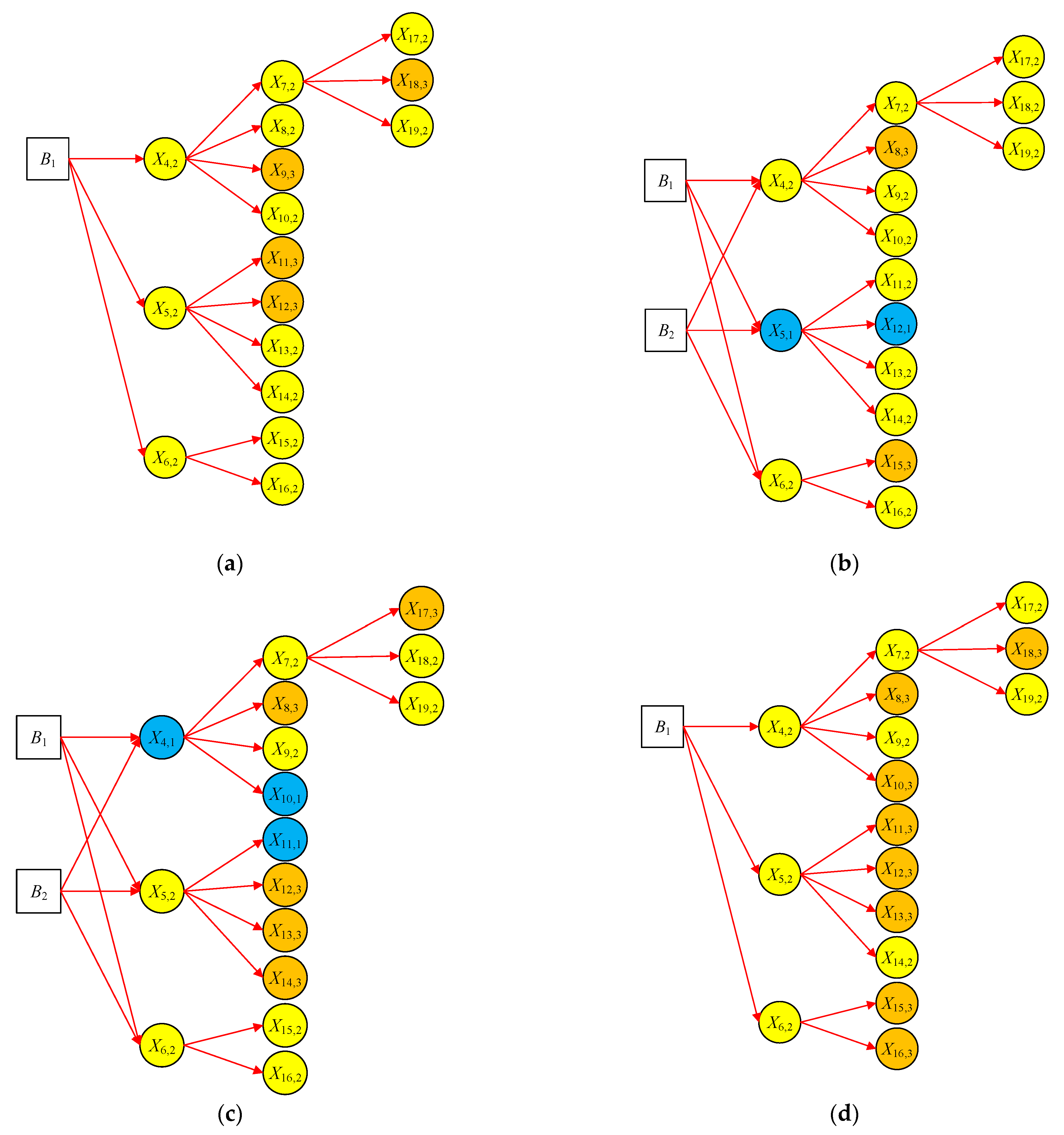
According to the example data in Table 5, the value range of each variable in Table 3 was used to determine the state of the variable under each piece of evidence. In the DUCG, yellow represents state 2, orange represents state 3, and blue represents state 1. Figure 6 can be converted into Figure 9.
After the state of the variable was determined, based on the conditional events in Table 4, the state of the unknown variable in Figure 9 was determined and then simplified according to DUCG simplification rules. During simplification, the action events that met the conditions were indicated by a solid red line, as shown in Figure 10.
In Figure 10a,d, only B1 is simplified, i.e., the evaluation results of Changning and Jiaoshiba were shale-gas exploration and development target areas (level I areas).
In Figure 10b,c, B1 and B3 are simplified, respectively. The possible hypotheses were calculated as given below.
In Figure 10b, we have:
H2,1 = B2,1 and H1,1 = B1,1; therefore,
Calculated according to Equation (2),
According to Equation (3), the sorting probability is obtained as follows:
The final evaluation results are shown in Table 6.
The evaluation results of sequence analysis methods are shown in Table 7 [14]. This method was evaluated by the experts’ scoring indicators. Both the DUCG and sequence analysis methods as evaluation methods introduced expert experience knowledge. The evaluation results were consistent and were divided into target, favorable, and prospective areas. However, only evaluation scores and conclusions were given in sequence analysis methods and the probability value of the evaluation result could not be calculated. Because of the uncertainty of the evaluation results in the field of reservoir engineering, probability can better play an auxiliary role as the evaluation result for reservoir experts in the evaluation of shale-gas sweet spot. Regarding the value ranges of different evaluation indicators selected by various experts, the DUCG can provide the probability value of the evaluation results and a reference strictly based on probability theory for the later stage of reservoir exploration and development test simulation. In addition, in terms of knowledge representation, the results scored by experts in sequence analysis methods can be used as the basis for the causality in the DUCG, i.e., the output of sequence analysis methods can be used as the input for the DUCG.
4.2. Results from Incomplete Data
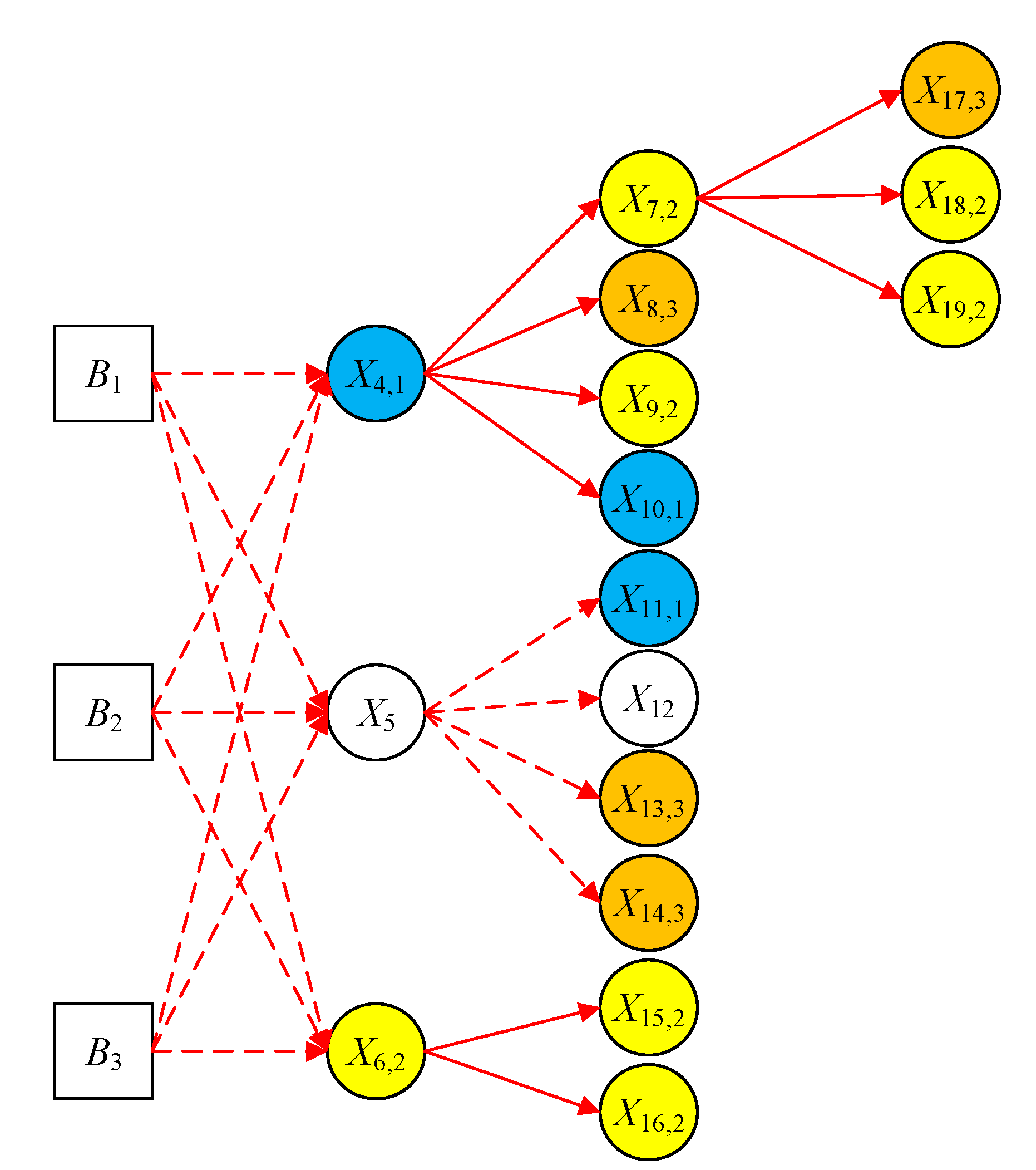
In some cases, the values of evaluation indicators cannot be obtained. For example, another set of data in Fushun-Yongchuan is shown in Table 8, where the pressure coefficient (X12) is unknown. In this case, the sweet spot was evaluated when the evidence was incomplete.
According to Table 8, evidence E5 = E8,4E9,2E10,1E11,1E13,3E14,3E15,2E16,2E17,3 E18,2E19,2 and the conditional event in Table 4 could be converted from Figure 6 to Figure 11. The state of variable X9 in Figure 11 was unknown, so the conditional event between X5 and its child variables could not be determined. In the DUCG, if the state of the variable in the conditional event is unknown, the graph structure cannot be determined. At this time, the prior probability of the effective state of the variable must be given or calculated in some way. Note that if state k of X12 is given, the state of X5 and the conditional events with child variables X11, X12, X13, and X14 can be determined. Similarly, whether the conditional event between B1, B2, B3 and X4, X5, X6 is true and the entire evaluation model can also be determined. According to E5, Pr{X12,k} was calculated, which is more objective than directly providing Pr{X12,k}. When the conditional event Z is not observed, the prior distribution of Z can be expanded in the form of a full combination [22]. However, when the graph results are complex and there are many conditional events, this method expression is not clear enough and the calculation is large.
This paper proposed a weighted-graph method to solve the above problems: X12 has three states in Table 3; for each state, the evaluation model was different (or the same, the specific depending on the conditional event). The weighted graphs were generated according to each state of X12. For each weighted graph, the possible evaluation results were obtained, and then the evaluation results of all weighted graphs were added to obtain the total evaluation result. If there were multiple variables in the condition event whose states were unknown, their possible states were combined and each state in the state combination then corresponded to a weighted graph. Lastly, the possible evaluation results were produced according to each weighted graph.
When experts have different opinions on the selection of evaluation indicators in the evaluation model or the value range of evaluation indicators, the concept of a weighted graph can be adopted, i.e., the knowledge system of an expert is used as a weighted graph, and each weighted graph is determined. The weight is calculated by a certain method or directly given, according to the authority of the expert, and the evaluation results of all weighted graphs are combined to obtain the total evaluation result.
We used evidence E5 as an example to show the calculation method in the case of subgraphs.
In E5, the state of X12 is not given and there are three possible states for X12 to be considered. This needs to be divided into three subgraphs. When X12 is in state 1, DUCG1 denotes subgraph 1 and ω1 = Pr{X12,1} denotes the probability of DUCG1. When X12 is in state 2, DUCG2 denotes subgraph 2 and ω2 = Pr{X12,2} denotes the probability of DUCG2. When X12 is in state 3, DUCG3 denotes subgraph 3 and ω3 = Pr{X12,3} denotes the probability of DUCG3. The divided subgraphs are shown in Figure 12.
In Figure 12a, B1 is isolated under evidence E5 because certain conditional events are not true. In Figure 12b,c, B3 is isolated and these variables are deleted under the simplified DUGG rule. The reasoning process of the DUCG adds the operation of dividing the weighted graph before it is simplified in the case of incomplete data. According to Equation (4), in Figure 12, E5 is expanded in DUCG1, DUCG2, and DUCG3:
In DUCG1, we have:
In DUCG2, we have:
In DUCG3, we have:
The combined calculation is as follows:
Lastly, Hkj is ranked by probability:
Evaluation results: The probability of belonging to the target area, the favorable area, and a prospective area was 27.03%, 46.26%, and 26.71%, respectively.
In the case of incomplete evaluation index data, it is difficult for other evaluation methods to obtain relatively accurate and justified evaluation results. The DUCG method does not depend on data, using expert knowledge instead, and can model various complex uncertain causality relationships and produce a precise reasoning. Using the graphical representation, the reasoning process in Figure 12 is intuitively demonstrated. This explains the results of the evaluation better.
5. Conclusions
This study proposed a DUCG method for shale-gas sweet-spot evaluation. According to the characteristics of shale-gas exploration and development, this study selected appropriate evaluation indicators from geological, engineering, and economic factors and determined the causality and causality function parameters between evaluation factors with the help of authoritative research results and expert knowledge in oil and gas reservoir engineering. In addition, the existing DUCG was extended: (1) multiple conditional events Znk;ij were proposed to satisfy the complex causality between evaluation indicators and (2) a weighted graph was created for the uncertain evidence of conditional events and comprehensive multiple-expert knowledge. Finally, the evaluation model was verified using data examples of typical shale-gas sweet spots. The results demonstrated that compared with other methods, the evaluation model based on the DUCG does not depend on data, its reasoning results are accurate, and the reasoning process can be graphically presented, making its conclusion more objective, credible, and explanatory.
In future work, we will select more representative unconventional reservoir desert areas for model construction, synthesize more expert experience, and use actual reservoir areas to verify in order to create a more comprehensive and accurate evaluation model.
Author Contributions
Conceptualization, Q.Y., B.Y. and Q.Z.; methodology, Q.Z. and Q.Y.; software, Q.Y.; validation, B.Y. and Q.Y.; formal analysis, Q.Y.; investigation, B.Y. and Q.Y.; resources, B.Y. and Q.Y.; data curation, B.Y. and Q.Y.; writing—original draft preparation, B.Y. and Q.Y.; writing—review and editing, B.Y. and Q.Y.; visualization, Q.Y.; supervision, Q.Z.; project administration, Q.Z. All authors have read and agreed to the published version of the manuscript.
Funding
This research was supported by Institute for Guo Qiang, Tsinghua University (project number: 2020QG0001) and Langfang Science and technology support Program (project number: 2021013071).
Institutional Review Board Statement
Not applicable.
Informed Consent Statement
Not applicable.
Data Availability Statement
The study did not report any data.
Conflicts of Interest
The authors declare no conflict of interest.
References
- Song, Z.; Xu, X.; Wang, B.; Zhao, L.; Yang, G.; Qiu, Q. Advances in shale gas resource assessment methods and their future evolvement. Oil Gas Geol. 2020, 41, 1038–1047. [Google Scholar]
- Zhiliang, H.E.; Haikuan, L.I.E.; Tingxue, J.I.A.N.G. Challenges and countermeasures of effective development with large scale of deep shale gas in Sichuan Basin. Reserv. Eval. Dev. 2021, 11, 1–11. [Google Scholar]
- He, X. Sweet spot evaluation system and enrichment and high yield influential factors of shale gas in Nanchuan area of eastern Sichuan Basin. Nat. Gas Ind. 2021, 41, 59–71. [Google Scholar]
- Wang, S.; Shi, C.; Wang, J. New equations for characterizing water flooding in ultra-high water-cut oilfields. Oil Gas Geol. 2020, 41, 1282–1287. [Google Scholar]
- Zhang, X.; Zhang, M.; Yang, L.; Yang, L.; Zhang, Y.; Zhou, Y. Improved Calculation Method for Shale Gas Reserves. Contemp. Chem. Ind. 2021, 50, 1450–1454. [Google Scholar]
- Jiang, J.; Tomin, P.; Zhou, Y. Inexact methods for sequential fully implicit (SFI) reservoir simulation. Comput. Geosci. 2021, 1–22. [Google Scholar] [CrossRef]
- Zhou, Y.; Zhao, A.; Yu, Q.; Zhang, D.; Zhang, Q.; Lei, Z. A new method for evaluating favorable shale gas exploration areas based on multi-linear regression analysis: A case study of marine shales of Wufeng-Longmaxi Formations, Upper Yangtze Region. Sediment. Geol. Tethyan Geol. 2021, 1–13. [Google Scholar] [CrossRef]
- Chen, G.; Sun, A.; Tang, H.; Tang, C. Water cut predication of water flood oilfield by the application of combined model. Reserv. Eval. Dev. 2016, 6, 11–13+18. [Google Scholar]
- Li, J.; Liu, X.; Shang, B.; Wang, D.; Gao, Z. Study on quantitative reservoir characterization based on geological risk. Xinjiang Oil Gas 2021, 17, 3–4, 50–52, 77. [Google Scholar]
- Zhong, Y.; Wang, S.; Luo, L.; Yang, J.; Qiu, Y. Knowledge Mining for Oilfield Development Index Prediction Model Using deep learning. J. Southwest Pet. Univ. 2020, 42, 63–74. [Google Scholar]
- Otchere, D.; Ganat, A.; Gholami, R.; Ridha, S. Application of supervised machine learning paradigms in the prediction of petrole-um reservoir properties: Comparative analysis of ANN and SVM models. J. Pet. Sci. Eng. 2021, 200, 108182. [Google Scholar] [CrossRef]
- Wang, S.; Li, J.; Guo, Q.; Li, D. Application of AHP Method to Favorable Area Optimization for Tight Oil: A Case Study in Daanzhai Formation, Jurassic, Central of the Sichuan Basin. Adv. Earth Sci. 2015, 30, 715–723. [Google Scholar]
- Shang, Y. Application of the analytic hierarchy process in the low-grade reserves evaluation. Pet. Geol. Oilfield Dev. Daqing 2014, 33, 55–59. [Google Scholar]
- Guan, Q.; Dong, D.; Wang, Y.; Huang, J.; Wang, S. AHP Application to Shale Gas Exploration Areas Assessment in Sichuan Basin. Bull. Geol. Sci. Technol. 2015, 34, 91–97. [Google Scholar]
- Zhang, Q.; Dong, C.; Cui, Y.; Yang, Z. Dynamic Uncertain Causality Graph for Knowledge Representation and Probabilistic Reasoning: Statistics Base, Matrix, and Application. IEEE Trans. Neural Netw. Learn. Syst. 2014, 25, 645. [Google Scholar] [CrossRef] [PubMed]
- Zhou, Z.; Qin, Z. Model Event/Fault Trees with Dynamic Uncertain Causality Graph for Better Probabilistic Safety Assessment. IEEE Trans. Reliab. 2017, 66, 178–188. [Google Scholar] [CrossRef]
- Dong, C.; Zhou, Z.; Zhang, Q. Cubic Dynamic Uncertain Causality Graph: A New Methodology for Modeling and Reasoning about Complex Faults with Negative Feedbacks. IEEE Trans. Reliab. 2018, 67, 920–932. [Google Scholar] [CrossRef]
- Jiao, Y.; Zhang, Z.; Zhang, T.; Shi, W.; Hu, J.; Zhang, Q. Development of an artificial intelligence diagnostic model based on dynamic uncertain causality graph for the differential diagnosis of dyspnea. Front. Med. 2020, 14, 488–497. [Google Scholar] [CrossRef]
- Ning, D.; Zhang, Z.; Qiu, K.; Lu, L.; Zhang, Q.; Zhu, Y.; Wang, R. Efficacy of intelligent diagnosis with a dynamic uncertain causality graph model for rare disorders of sex development. Front. Med. 2020, 14, 498–505. [Google Scholar] [CrossRef]
- Dong, C.; Wang, Y.; Zhou, J.; Zhang, Q.; Wang, N.; Faes, L. Differential Diagnostic Reasoning Method for Benign Paroxysmal Positional Vertigo Based on Dynamic Uncertain Causality Graph. Comput. Math. Methods Med. 2020, 2020, 1541989. [Google Scholar] [CrossRef]
- Zhang, Q.; Bu, X.; Zhang, M.; Zhang, Z.; Hu, J. Dynamic uncertain causality graph for computer-aided general clinical diagnoses with nasal obstruction as an illustration. Artif. Intell. Rev. 2021, 54, 27–61. [Google Scholar] [CrossRef]
- Zhang, Q. Dynamic Uncertain Causal Graph for knowledge repressntation and reasoning: Discrete DAG cases. J. Comput. Sci. Technol. 2012, 27, 1–23. [Google Scholar] [CrossRef]
- Zhang, Q.; Geng, S. Dynamic uncertain causality graph applied to dynamic fault diagnoses of large and complex systems. IEEE Trans. Reliab. 2015, 64, 910–927. [Google Scholar] [CrossRef]
- Wang, M.; Li, J.; Ye, J. Shale Gas Knowledge Book; Science Press: Beijing, China, 2012; pp. 30–32. [Google Scholar]
- Li, D. China’s Multicycle Superimposed Petroliferous Basins: Theory and Explorative Practices. Xinjiang Pet. Geol. 2013, 34, 497–503. [Google Scholar]
- Bao, H.; Liu, X.; Zhou, Y.; Yang, Y.; Guo, X. Favorable Area and Potential Analyses of Tight Oil in Jimsar Sag. Spec. Oil Gas Reserv. 2016, 23, 38–42, 152. [Google Scholar]
- Yang, Z.; Hou, L.; Tao, S.; Cui, J.; Wu, S.; Lin, S.; Pan, S. Formation conditions and “sweet spot” evaluation of tight oil and shale oil. Pet. Explor. Dev. 2015, 42, 555–565. [Google Scholar]
Figure 1.
DUCG example.

Figure 2.
Logic gate specification (LGS6).

Figure 3.
Illustration of the DUCG model.

Figure 4.
Example of a conditional case.

Figure 5.
Causality analysis of the evaluation model for shale-gas sweet spots.

Figure 6.
Shale-gas sweet-spot evaluation model with the DUCG.

Figure 7.
Child variable combination of target area evaluation: (a) Z4,2;1,1 = X5,2X6,2; (b) Z4,2;1,1 = X5,1X6,2; (c) Z4,2;1,1 = X5,2X6,1.
Figure 7.
Child variable combination of target area evaluation: (a) Z4,2;1,1 = X5,2X6,2; (b) Z4,2;1,1 = X5,1X6,2; (c) Z4,2;1,1 = X5,2X6,1.

Figure 8.
Causality function parameters of the variables in Figure 6.
Figure 8.
Causality function parameters of the variables in Figure 6.

Figure 9.
Evaluation models of shale-gas sweet spots with E in (a) Changning with E1, (b) Weiyuan with E2, (c) Fushun-Yongchuan with E3, and (d) Jiaoshiba with E4.
Figure 9.
Evaluation models of shale-gas sweet spots with E in (a) Changning with E1, (b) Weiyuan with E2, (c) Fushun-Yongchuan with E3, and (d) Jiaoshiba with E4.

Figure 10.
Simplified evaluation model of shale-gas sweet spots in (a) Changning with E1, (b) Weiyuan with E2, (c) Fushun-Yongchuan with E3, and (d) Jiaoshiba with E4.
Figure 10.
Simplified evaluation model of shale-gas sweet spots in (a) Changning with E1, (b) Weiyuan with E2, (c) Fushun-Yongchuan with E3, and (d) Jiaoshiba with E4.

Figure 11.
Evaluation model of Fushun-Yongchuan in E5.

Figure 12.
Subgraphs of X12 in different states with E5, listed as (a) DUCG1, (b) DUCG2, and (c) DUCG3.
Figure 12.
Subgraphs of X12 in different states with E5, listed as (a) DUCG1, (b) DUCG2, and (c) DUCG3.


Table 1.
Relevant industry standards.
| Relevant Industry Standard | Standard Number | State |
|---|---|---|
| Method of geological evaluation of natural-gas reserves | SY/T 5601-2009 | Current |
| Technical requirements for economic evaluation of gas field development and adjustment programs | SY/T 6177-2009 | Current |
| Evaluation method of oil and gas reservoirs | SY/T 6285-2011 | Current |
Table 2.
Shale-gas evaluation criteria and main indicators.
| Sweet Spot | Evaluation Indicator | Target Area | Favorable Area | Prospecting Area |
|---|---|---|---|---|
| Geological sweet spot | Thickness of organic-rich shale/m | >50 | 50–30 | <30 |
| Total organic carbon (TOC)/% | >4 | 4–2 | <2 | |
| Maturity of organic matter (Ro)/% | 1.1–2.5 | 2.5–4 | >4 | |
| Favorable area/km2 | >2500 | 2500–1000 | <1000 | |
| Gas content/(m3·t−1) | >4 | 4–2 | <2 | |
| Tectonic setting | Anticline normal structure | Slope | Syncline negative structure | |
| Engineering sweet spot | Burial depth/km | 1.5–3.5 | 0.5–1.5 | <0.5 or 3.5–4.5 |
| Pressure factor | >1.3 | 1.0–1.3 | <1.0 | |
| Degree of natural cracks | Full development | Interlayer seam development | No development | |
| Surface condition | Plains and hills | Mountains or dams | Lakes or valleys | |
| Economic sweet spot | Market demand | Demand exceeds supply | Balance between supply and demand | Supply exceeds demand |
| Infrastructure | In a pipe network | Close to a pipe network | Away from a pipe network |
Table 3.
Variables in the evaluation model of shale-gas sweet spots.
| Name | Description | State and State Description |
|---|---|---|
| B1 | Shale-gas target area | 0: false; 1: true |
| B2 | Shale-gas favorable area | 0: false; 1: true |
| B3 | Shale-gas prospective area | 0: false; 1: true |
| X4 | Geological sweet spot | 0: false; 1: common; 2: good |
| X5 | Engineering sweet spot | 0: false; 1: common; 2: good |
| X6 | Economic sweet spot | 0: false; 1: common; 2: good |
| X7 | Organic matter | 0: unknown; 1: common; 2: good |
| X8 | Favorable area (km2) | 0: unknown; 1: <1000; 2: >1000 and <2500; 3: >2500 |
| X9 | Gas content (m3·t−1) | 0: unknown; 1: <2; 2: 2–4; 3: >4 |
| X10 | Tectonic setting | 0: unknown; 1: syncline negative structure; 2: slope; 3: anticline normal structure |
| X11 | Burial depth (km) | 0: unknown; 1: <0.5 or 3.5–4.5; 2: 0.5–1.5; 3: 1.5–3.5 |
| X12 | Pressure factor | 0: unknown; 1: <1.0; 2: 1.0–1.3; 3: >1.3 |
| X13 | Degree of natural cracks | 0: unknown; 1: undeveloped; 2: interlayer seam development; 3: fully developed |
| X14 | Surface condition | 0: unknown; 1: lakes or valleys; 2: mountains or dams; 3: plains and hills |
| X15 | Market demand | 0: unknown; 1: supply exceeds demand; 2: balanced; 3: demand exceeds supply |
| X16 | Infrastructure | 0: unknown; 1: away from a pipe network; 2: close to a pipe network; 3: in a pipe network |
| X17 | Thickness of organic-rich shale (m) | 0: unknown; 1: <30; 2: 30–50; 3: >50 |
| X18 | Total organic carbon (%) | 0: unknown; 1: <2; 2: 2–4; 3: >4 |
| X19 | Organic maturity (%) | 0: unknown; 1: >4; 2: 2–4; 3: 1.1–2.5 |
Table 4.
Condition event list of the shale-gas evaluation model.
| No. | Parent Variable | List or Description of Condition Events |
|---|---|---|
| 1 | B1,1 | Z4,2;1,1 = X5,2X6,2 + X5,1X6,2 + X5,2X6,1 Z4,1;1,1 = X5,2X6,2 Z5,2;1,1 = X4,2X6,2 + X4,2X6,1 + X4,1X6,2 Z5,1;1,1 = X4,2X6,2 Z6,2;1,1 = X4,2X5,2 + X4,2X5,1 + X4,1X5,2 Z6,1;1,1 = X4,2X5,2 |
| 2 | B2,1 | Z4,2;2,1 = X5,1X6,2 + X5,2X6,1 + X5,1X6,1 Z4,1;2,1 = X5,2X6,2 + X5,2X6,1 + X5,1X6,2 Z5,2;2,1 = X4,2X6,1 + X4,1X6,2 + X4,1X6,1 Z5,1;2,1 = X4,2X6,2 + X4,2X6,1 + X4,1X6,2 Z6,2;2,1 = X4,2X5,1 + X4,1X5,2 + X4,1X5,1 Z6,1;2,1 = X4,2X5,2 + X4,2X5,1 + X4,1X5,2 |
| 3 | B3,1 | Z4,1;3,1 = X5,1X6,1 + X5,2X6,1 + X5,1X6,2 Z4,2;3,1 = X5,1X6,1 Z5,1;3,1 = X4,1X6,1 + X4,1X6,2 + X4,2X6,1 Z5,2;3,1 = X4,1X6,1 Z6,1;3,1 = X4,1X5,1 + X4,1X5,2 + X4,2X5,1 Z6,2;3,1 = X4,1X5,1 |
| 4 | X4,2 | All child variables of X4 are in state 2 or 3. |
| 5 | X4,1 | |
| 6 | X5,2 | All child variables of X5 are in state 2 or 3, or X11 is state 1, and two of the other three variables are in state 3. |
| 7 | X5,1 | |
| 8 | X6,2 | All child variables of X6 are in state 2 or 3. |
| 9 | X6,1 | |
| 10 | X7,2 | All child variables of X7 are in state 2 or 3. |
| 11 | X7,1 |
Table 5.
Shale-gas data of four areas in the Sichuan basin.
| Evaluation Indicator | Changning (E1) | Weiyuan (E2) | Fushun-Yongchuan (E3) | Jiaoshiba (E4) |
|---|---|---|---|---|
| Thickness of organic-rich shale (X17) | 33–46 | 40–50 | 60–100 | 38–44 |
| Total organic carbon (X18) | 1.9–7.3/4.0 | 1.9–6.4/2.7 | 1.6–6.8/3.8 | 1.5–6.1/3.5 |
| Organic maturity (X19) | 2.6 | 2.7 | 2.5–3.0 | 2.6 |
| Favorable area (X8) | 2050 | 4216 | 3900 | 5450 |
| Gas content (X9) | 4.1 | 2.92 | 3.6 | 3.5 |
| Tectonic setting (X10) | Slope | Slope | Syncline negative structure | Anticline normal structure |
| Burial depth (X11) | 2.3–3.2 | 1.3–3.7 | 3.2–4.5 | 2.4–3.5 |
| Pressure factor (X12) | 1.35–2.03 | 0.92–1.77 | 2.0–2.25 | 1.35–1.55 |
| Degree of natural cracks (X13) | Interlayer seam development | Interlayer seam development | Full development | Full development |
| Surface condition (X14) | Mountains or dams | Mountains or dams | Plains or hills | Mountains or dams |
| Market demand (X15) | Medium | Larger | Medium | Larger |
| Infrastructure (X16) | Close to a pipe network | Close to a pipe network | Close to a pipe network | In a pipe network |
Table 6.
Evaluation results of Table 5.
Table 6.
Evaluation results of Table 5.
| Area | Target Area (Level I) | Favorable Area (Level II) | Prospective Area (Level III) |
|---|---|---|---|
| Jiaoshiba | 100% | ||
| Changning | 100% | ||
| Fushun-Yongchuan | 51.51% | 48.49% | |
| Weiyuan | 41.49% | 58.51% |
Table 7.
Results of grading and classification of four regional sequence analysis methods.
| Area | Score | Rank | Level |
|---|---|---|---|
| Jiaoshiba | 72.7670 | 1 | I |
| Changning | 72.2571 | 2 | I |
| Fushun-Yongchuan | 71.3968 | 3 | II |
| Weiyuan | 67.9926 | 4 | III |
Table 8.
Data on the oil layer group in Fushun-Yongchuan.
| Evaluation Indicator | Variable | Data |
|---|---|---|
| Thickness of organic-rich shale | X17 | 60–100 |
| Total organic carbon | X18 | 1.6–6.8/3.8 |
| Organic maturity | X19 | 2.5–3.0 |
| Favorable area | X8 | 3900 |
| Gas content | X9 | 3.6 |
| Tectonic setting | X10 | Syncline negative structure |
| Burial depth | X11 | 3.2–4.5 |
| Pressure factor | X12 | — |
| Degree of natural cracks | X13 | Fully developed |
| Surface condition | X14 | Plains and hills |
| Market demand | X15 | Balance between supply and demand |
| Infrastructure | X16 | Close to a pipe network |
Publisher’s Note: MDPI stays neutral with regard to jurisdictional claims in published maps and institutional affiliations. |
© 2021 by the authors. Licensee MDPI, Basel, Switzerland. This article is an open access article distributed under the terms and conditions of the Creative Commons Attribution (CC BY) license (https://creativecommons.org/licenses/by/4.0/).
Share and Cite
MDPI and ACS Style
Yao, Q.; Yang, B.; Zhang, Q. Dynamic Uncertain Causality Graph Applied to the Intelligent Evaluation of a Shale-Gas Sweet Spot. Energies 2021, 14, 5228. https://0-doi-org.brum.beds.ac.uk/10.3390/en14175228
AMA Style
Yao Q, Yang B, Zhang Q. Dynamic Uncertain Causality Graph Applied to the Intelligent Evaluation of a Shale-Gas Sweet Spot. Energies. 2021; 14(17):5228. https://0-doi-org.brum.beds.ac.uk/10.3390/en14175228
Chicago/Turabian StyleYao, Quanying, Bo Yang, and Qin Zhang. 2021. "Dynamic Uncertain Causality Graph Applied to the Intelligent Evaluation of a Shale-Gas Sweet Spot" Energies 14, no. 17: 5228. https://0-doi-org.brum.beds.ac.uk/10.3390/en14175228
Note that from the first issue of 2016, this journal uses article numbers instead of page numbers. See further details here.