Mathematical Modelling of Transient Processes in an Asynchronous Drive with a Long Shaft Including Cardan Joints

Abstract

Beginning with the classic methods, a mathematical model of an electromechanical system is developed that consists of a deep bar cage induction motor that, via a complex motion transmission with distributed mechanical parameters, drives a working machine, loading the drive system with a constant torque. The electromagnetic field theory serves to create the motor model, which allows addressing the displacement of current in the rotor cage bars. Ordinary and partial differential equations are used to describe the electromechanical processes of energy conversion in the motor. The complex transmission of the drive motion consists of a long shaft with variable geometry cardan joints mounted on its ends. Non-linear electromechanical differential equations are presented as a system of ordinary differential equations combined with a mixed problem of Dirichlet first-type and Poincaré third-type boundary conditions. This system of equations is integrated by discretising partial derivatives by means of the straight-line methods and successive integration as a function of time using the Runge–Kutta fourth-order method. Starting from there, complicated transient processes in the drive system are analysed. Results of computer simulations are presented in the graphic form, which is analysed.

1. Introduction

Mathematical modelling of transient processes in asynchronous drives is important at the stages of both design and operation. It concerns physical effects in motion transmission, where a drive motor’s torque is transferred to a load system. When the distance between the drive motor and the load system is substantial, the torque is determined by describing a long shaft in a distributed mechanical parameters system [1,2,3,4,5,6]. Points of power receipt can obviously have varying practical configurations, which may in turn complicate kinematic and drive system equations. Drives deserve attention where the axes of an output motor drive shaft and working machine shaft are not aligned. In the circumstances, the problem of adding a static pair of reduction gears arises, which requires a constant angle between the shaft axes, on the one hand, and complicates the system’s design on the other. For instance, these cases of non-aligned shafts occur in rolling mill drives [7,8].

Drive systems including cardan joints are free from this shortcoming of non-aligned shafts [9,10,11]. A cardan joint is a mechanical element serving to transmit torque and normally used to connect driving and driven shafts that cannot be connected directly due to the distance or the need to allow some relative motion between them. The theory of applied mechanics implies that rather complicated motions are present in drive systems containing cardan joints. This is caused by the different instantaneous rotational speeds of co-working and interconnected shafts, which results in their different rotation angles [12,13]. In the end, this causes a change of the cardan joint’s speed ratio.

Equal rotational speeds of a driving machine’s cardan joints and a driven working machine rotor are the key requirement of motion transmission in precise drive systems. Control systems in precise drives use information from a variety of rotational speed and shaft rotation angle sensors. The information from these sensors is transmitted to a microprocessor and then processed into input signals of drive motor control. Since the speed ratios in such systems are variable, the issue arises of correct signal identification in control systems of entire electric drives [4,14].

To prevent these problems, odd numbers of shafts, that is, even numbers of cardan joints, are installed in precise drives. Only in this case can identical speeds of rotor shafts of a drive system and a loading working machine be attained. A series of requirements need to be met to assure identical speeds, which will be discussed in this paper.

It should be pointed out that we analyse drive systems with long shafts of susceptible motion transmission. This means that not only values of variable speed ratios but also oscillatory processes across the long shaft need to be considered. Addressing these phenomena evidently complicates the process of motor control in drive systems even further.

The article [3] describes drive systems containing long and flexible shafts that are very sensitive to torsional vibrations where their natural frequencies act on the external torque applied to a shaft. Torsion analysis is required by international standards to evaluate the reliability of shaft operation all the entire range of motor speeds. The possible interactions between the torque produced by an induction motor and the frequencies of a driven shaft are one of the hardest engineering problems. At the stage of design, torsional analysis is required to evaluate a shaft’s durability on the basis of harmonic values of the electromagnetic torque in the motor’s air gap [15,16,17].

Models including rotating shafts are built with fixed rigid mutual connections between a number of inertias. They make up a multiresonant system with its own frequencies that can be excited. A shaft excited with externally applied forces is subject to faster wear or damage [18], which may affect industrial productivity. Harmonic voltages and currents can generate pulsing torque pulsing torque components. Some of these components may be relatively high [19]. If some of these pulsing torques have frequencies close to the frequencies of a shaft’s own vibrations, they can increase the shear stress in the shaft material above its design value.

In many industrial systems, the coupling of the working machine to the drive is carried out by a long transmission shaft. In such cases, non-linear mechanical vibrations occur, including torsional vibrations, which can be described in a simplified manner with the model of a dual-mass system [20]. Mechanical vibrations negatively affect the operation of drive systems and complicate the analysis of the control system [21]. The problem is especially complicated in resonant and near-resonance states. In such cases, the control system, with various disturbances occurring, should avoid mechanical oscillations, which may even lead to damage to the drive system components.

A mathematical model of a susceptible motion transmission-based asynchronous drive including the distributed mechanical parameters of a long shaft that contains cardan joints is the chief purpose of our paper. Based on this model, we analyse transient oscillatory electromechanical processes in the drive.

2. Drive Systems Including Cardan Joints

We analyse one of the most commonly used drive systems that contains cardan joints with a susceptible three-shaft motion transmission and two swivels. The first driving shaft of the asynchronous machine rotor is absolutely rigid. The second, central, susceptible shaft is described with equations of distributed mechanical parameters. The third shaft, the input shaft of the loading working machine, is absolutely rigid, similar to the first shaft. Figure 1 shows a kinematic diagram of a drive transmission system including a susceptible long shaft and cardan joints.

The following terminology is introduced to Figure 1: M_EM—electromagnetic torque of the drive motor, M_O—drive loading torque, J_EM—moment of inertia of the drive motor, J_O—total moment of load inertia, ω_EM—angular velocity of the rotor, ω_O—angular load rotor velocity, φ_j, ω_j (j = 1, 2, …, N)—the angle of rotation and the angular velocity of the long shaft discretisation element, i_1,2—speed ratio of the first cardan joint toward the motor, i_2,3—speed ratio of the second cardan joint toward the load, α_1,2, α_2,3—angles between the shafts connected with cardan joints.

Such a system can reach a state where the rotational speeds of the first and third shafts are identical, which is possible in the presence of a resultant speed ratio with a value of one. These are the conditions necessary for equal rotational speeds of the first and third shafts [12]:

• Identical angles between axes of the first and middle shafts and the third and middle shafts;
• Planes of the fork-articulated endings of the middle (second) shaft are mutually shifted in space by an angle of π/2;
• Axes of the three shafts are situated in the same plane or with identical angle projections on the middle shaft’s plane.

These three prerequisites restrict the application of similar motion transmissions to drive systems. They are very rare, and cardan joints can be successfully installed in most drive systems. Their use is additionally limited by the maximum angles between shafts connected with a cardan joint.

Dynamic angle changes between co-working, connected shafts strongly argue for the application of cardan joints, which are used in ship drives, rolling mills, or automobiles [22,23]. For this reason, modelling and analysis of transient states in drive systems that include susceptible motion transmissions including cardan joints is very topical [9,10,11]. In some cases of rotational systems operating in difficult conditions, a mathematical model of motion transmission should be analysed addressing a variety of latent motions, both internal and external [4].

In drive systems including long shafts, the susceptibility of these elements in distributed parameter systems must be additionally taken into consideration [4,6,24,25,26]. Only the susceptibility of the middle shaft needs to be addressed in our system, since it is several times longer than the first or third shaft. Introduction of the second (middle) shaft susceptibility causes the appearance of a mutual spatial shift of planes of fork shaft endings; as a result, the rotational speeds of the first and third shafts will not be the same [10]. This is an adverse effect, especially in precise control systems where signals from a rotational speed sensor are supplied to drive motors [27,28,29,30], for instance, in PMSM and BLDC motors.

The development of a mathematical model of a long-shaft asynchronous drive including cardan joints is approached with an interdisciplinary method that modifies the Hamilton–Ostrogradsky integral variational principle by expanding the Lagrangian with two components: dissipation energy and energy of non-potential external forces [27,31]. This method enables the development of mathematical models not only for lumped parameter systems but also the modelling of complicated dynamic systems of both lumped and distributed parameters. This extends the applicability of the modified Hamilton–Ostrogradsky principle to a range of interdisciplinary fields of science. This is the starting point for our mathematical models of all the asynchronous drive elements.

3. Mathematical Model of Motion Transmission

The model of the system in Figure 1 is based on kinematic equations considering a cardan joint for the two-shaft scenario shown in Figure 2 [12].

The following terminology is introduced to Figure 2: ψ₁—rotation angle of the first shaft, ψ₂—rotation angle of the second shaft, ϖ₁, ϖ₂—angular shaft velocities, α_1,2—stationary angle between axes of both the shafts.

We will write the cardan joint system of equations as follows [12]:

$${\mathsf{\psi }}_2=\mathrm{arctg}\left(\frac{1}{\cos {\mathsf{\alpha }}_{1,2}}\mathrm{tg}{\mathsf{\psi }}_1\right).$$

(1)

The integration of (1) as a function of time t and rotation angle ψ₁ produces [12]:

$$\frac{{\mathsf{\varpi }}_2}{{\mathsf{\varpi }}_1}\equiv {\mathrm{i}}_{1,2}=\frac{1}{\cos {\mathsf{\alpha }}_{1,2}\left(1+{\mathrm{tg}}^2{\mathsf{\alpha }}_{1,2}{\sin }^2({\mathsf{\psi }}_1+\mathsf{\theta })\right)}\Rightarrow {\mathsf{\varpi }}_2=\frac{{\mathsf{\varpi }}_1}{\cos {\mathsf{\alpha }}_{1,2}\left(1+{\mathrm{tg}}^2{\mathsf{\alpha }}_{1,2}{\sin }^2({\mathsf{\psi }}_1+\mathsf{\theta })\right)},$$

(2)

where $\mathrm{i}$_1,2—cardan joint speed ratio, θ—an additional angle to address the mutual shift between axes of cardan joint fork endings.

If the dependence of the angle between the shafts is non-stationary, α_1,2(t) is a time function. Then, (2) will be expressed as follows [12]:

$${\mathsf{\varpi }}_2=\frac{{\mathsf{\varpi }}_1+0.5\mathrm{tg}{\mathsf{\alpha }}_{1,2}\sin 2({\mathsf{\psi }}_1+\mathsf{\theta }){\mathsf{\alpha }}_{1,2}^{\prime }}{\cos {\mathsf{\alpha }}_{1,2}\left(1+{\mathrm{tg}}^2{\mathsf{\alpha }}_{1,2}{\sin }^2({\mathsf{\psi }}_1+\mathsf{\theta })\right)},\frac{d{\mathsf{\alpha }}_{1,2}}{dt}\equiv {\mathsf{\alpha }}_{1,2}^{\prime }.$$

(3)

Figure 3 includes a transfer calculation diagram of an asynchronous drive including a susceptible long shaft.

The following additional terms are introduced in Figure 3: j—current discretisation node of shaft equations, ω_j—angular velocity of the jth discrete node, Δx—discretisation step, x—current coordinate, N—number of long shaft discretisation nodes.

If the long shaft is analysed as a dual mass system, all the parameters can be reduced to the drive motor in the general case. For a distributed parameter system, on the other hand, such a reduction of the shaft’s distributed parameters to the drive motor is not simple. To avoid this reduction, we suggest another approach: convert the motor’s mechanical parameters to the shaft’s left end and the load parameters to the shaft’s right end. Then, the system will be analysed in the coordinates of the susceptible shaft, that is, in a virtual system of coordinates. In the final analysis, one must move to a real, physical system of coordinates and to a system reduced to the motor’s rotor.

The wave equation [27,31] serves to model transmission with a long distributed parameter shaft:

$$\frac{{\partial }^2\mathsf{\phi }}{\partial t^2}=\frac{G}{\mathsf{\rho }}\frac{{\partial }^2\mathsf{\phi }}{\partial x^2}+\frac{\mathsf{\xi }}{\mathsf{\rho }{J}_P}\frac{{\partial }^3\mathsf{\phi }}{\partial x^2\partial t}=\frac{G}{\mathsf{\rho }}\frac{{\partial }^2\mathsf{\phi }}{\partial x^2}+\frac{\mathsf{\xi }}{\mathsf{\rho }{J}_P}\frac{{\partial }^2\mathsf{\omega }}{\partial x^2},\mathsf{\omega }=\frac{\partial \mathsf{\phi }}{\partial t}$$

(4)

where φ(x,t)—the shaft’s rotation angle, ω = $\partial$φ/$\partial$t—the shaft’s angular velocity, G—modulus of rigidity, ξ—coefficient of the shaft internal dispersion; ρ—density of the shaft material; J_P—the shaft’s polar moment of inertia.

Wave equations serve to model the motion transmission of the distributed parameter long-shaft drive system. Here, Poincaré third-type boundary conditions for (4) will be formulated on the basis of equality of electromagnetic torques, load, elasticity, and dissipation on the shaft ends according to d’Alembert law [32] considering values of cardan joint speed ratios:

$${\mathrm{i}}_{1,2}^{-2}{J}_{EM}{\frac{{\partial }^2\mathsf{\phi }}{\partial t^2}}_{|x=0}-G{J}_P{\left(\frac{\partial \mathsf{\phi }}{\partial x}\right)}_{|x=0}-\mathsf{\xi }{\left(\frac{\partial \mathsf{\omega }}{\partial x}\right)}_{|x=0}={\mathrm{i}}_{1,2}^{-1}{M}_{EM},$$

(5)

$${\mathrm{i}}_{2,3}^2{J}_O{\frac{{\partial }^2\mathsf{\phi }}{\partial t^2}}_{|x=L}+G{J}_P{\left(\frac{\partial \mathsf{\phi }}{\partial x}\right)}_{|x=L}+\mathsf{\xi }{\left(\frac{\partial \mathsf{\phi }}{\partial x}\right)}_{|x=L}={\mathrm{i}}_{2,3}{M}_O,$$

(6)

$${\mathrm{i}}_{1,2}=\frac{{\mathsf{\omega }}_1}{{\mathsf{\omega }}_{EM}},{\mathrm{i}}_{2,3}=\frac{{\mathsf{\omega }}_O}{{\mathsf{\omega }}_N},$$

(7)

where i_1,2—the first joint’s speed ratio in the shaft’s coordinates, i_2,3—the second joint’s speed ratio in the shaft’s coordinates (Figure 1).

The discretisation of (4)–(6) using the straight-line method produces:

$$\frac{{\partial }^2{\mathsf{\phi }}_i}{\partial t^2}\equiv \frac{\partial {\mathsf{\omega }}_i}{\partial t}=\frac{G}{\mathsf{\rho }}\frac{{\mathsf{\phi }}_{i-1}-2{\mathsf{\phi }}_i+{\mathsf{\phi }}_{i+1}}{{(\mathsf{\Delta }x)}^2}+\frac{\mathsf{\xi }}{\mathsf{\rho }{J}_p}\frac{{\mathsf{\omega }}_{i-1}-2{\mathsf{\omega }}_i+{\mathsf{\omega }}_{i+1}}{{(\mathsf{\Delta }x)}^2},i=1,2,\dots ,N,$$

(8)

$${\mathrm{i}}_{1,2}^{-2}{J}_{EM}\frac{d{\mathsf{\omega }}_1}{dt}-G{J}_p\frac{{\mathsf{\phi }}_2-{\mathsf{\phi }}_0}{2\mathsf{\Delta }x}-\mathsf{\xi }\frac{{\mathsf{\omega }}_2-{\mathsf{\omega }}_0}{2\mathsf{\Delta }x}={\mathrm{i}}_{1,2}^{-1}{M}_{EM},$$

(9)

$$-{\mathrm{i}}_{2,3}^2{J}_O\frac{d{\mathsf{\omega }}_N}{dt}+G{J}_p\frac{{\mathsf{\phi }}_{N+1}-{\mathsf{\phi }}_{N-1}}{2\mathsf{\Delta }x}+\mathsf{\xi }\frac{{\mathsf{\omega }}_{N+1}-{\mathsf{\omega }}_{N-1}}{2\mathsf{\Delta }x}={\mathrm{i}}_{2,3}{M}_O,$$

(10)

where φ₀, φ_N+1, ω₀, and ω_N+1—fictitious, virtual discretisation nodes of spatial derivatives [27].

Solving (8)—(10) together will result in:

$$\frac{d{\mathsf{\omega }}_1}{dt}=\frac{2\left({\mathrm{i}}_{1,2}^{-1}{M}_{EM}\mathsf{\Delta }x-J_{p}G({\mathsf{\phi }}_1-{\mathsf{\phi }}_2)-\mathsf{\xi }({\mathsf{\omega }}_1-{\mathsf{\omega }}_2)\right)}{\left(J_p\mathsf{\rho }\mathsf{\Delta }x+2{\mathrm{i}}_{1,2}^{-2}{J}_{EM}\right)\mathsf{\Delta }x},$$

(11)

$$\frac{d{\mathsf{\omega }}_i}{dt}=\frac{G}{\mathsf{\rho }}\frac{{\mathsf{\phi }}_{i-1}-2{\mathsf{\phi }}_i+{\mathsf{\phi }}_{i+1}}{{(\mathsf{\Delta }x)}^2}+\frac{\mathsf{\xi }}{\mathsf{\rho }{J}_p}\frac{{\mathsf{\omega }}_{i-1}-2{\mathsf{\omega }}_i+{\mathsf{\omega }}_{i+1}}{{(\mathsf{\Delta }x)}^2},i=2,\dots ,N-1,$$

(12)

$$\frac{d{\mathsf{\omega }}_N}{dt}=\frac{2\left(-{\mathrm{i}}_{2,3}^{}{M}_O\mathsf{\Delta }x+J_{p}G({\mathsf{\phi }}_{N-1}-{\mathsf{\phi }}_N)+\mathsf{\xi }({\mathsf{\omega }}_{N-1}-{\mathsf{\omega }}_N)\right)}{\left(J_p\mathsf{\rho }\mathsf{\Delta }x+2{\mathrm{i}}_{2,3}^2{J}_O\right)\mathsf{\Delta }x}.$$

(13)

Rotation angles and angular velocities of the rotor and input load shaft are calculated in the usual way for constant angles α_1,2 and α_2,3 from (1), (2):

$${\mathsf{\omega }}_{EM}={\mathsf{\omega }}_1\cos {\mathsf{\alpha }}_{1,2}\left(1+{\mathrm{tg}}^2{\mathsf{\alpha }}_{1,2}{\sin }^2{\mathsf{\phi }}_1\right),$$

(14)

$${\mathsf{\omega }}_O=\frac{{\mathsf{\omega }}_N}{\cos {\mathsf{\alpha }}_{2,3}\left[1+\mathrm{t}{\mathrm{g}}^2{\mathsf{\alpha }}_{2,3}{\sin }^2\left({\mathsf{\phi }}_N+\mathsf{\beta }-\mathsf{\gamma }\right)\right]},\mathsf{\beta }=\frac{\mathsf{\pi }}{2},$$

(15)

where γ—angle of shaft torsion, β—angle between planes of the shaft’s fork-articulated endings.

For non-stationary dependency between angles: α_1,2(t), α_2,3(t) = f(t) and time, see (3):

$${\mathsf{\omega }}_{EM}={\mathsf{\omega }}_1\cos {\mathsf{\alpha }}_{1,2}\left(1+{\mathrm{tg}}^2{\mathsf{\alpha }}_{1,2}{\sin }^2{\mathsf{\phi }}_1\right)-0.5\mathrm{tg}{\mathsf{\alpha }}_{1,2}\sin 2{\mathsf{\phi }}_1\frac{d{\mathsf{\alpha }}_{1,2}}{dt},$$

(16)

$${\mathsf{\omega }}_O=\frac{{\mathsf{\omega }}_N+0.5\mathrm{t}\mathrm{g}{\mathsf{\alpha }}_{2,3}\sin 2\left({\mathsf{\phi }}_N+\mathsf{\beta }-\mathsf{\gamma }\right)\frac{d{\mathsf{\alpha }}_{2,3}}{dt}}{\cos {\mathsf{\alpha }}_{2,3}\left[1+\mathrm{t}{\mathrm{g}}^2{\mathsf{\alpha }}_{2,3}{\sin }^2\left({\mathsf{\phi }}_N+\mathsf{\beta }-\mathsf{\gamma }\right)\right]},\mathsf{\beta }=\frac{\mathsf{\pi }}{2}.$$

(17)

The rotation angles of the rotor and input load shaft in the shaft coordinates will be found in the ordinary way:

$$\frac{d{\mathsf{\phi }}_{EM}}{dt}={\mathsf{\omega }}_{EM},\frac{d{\mathsf{\phi }}_O}{dt}={\mathsf{\omega }}_O.$$

(18)

4. Mathematical Model of the Motor

Since most medium and high-power asynchronous motors have enhanced starting torques, a deep bar cage asynchronous motor is analysed in our case. The theory of the electromagnetic field serves to address the skin effect in the rotor cage bars. The unknown function u_R—voltage drop across the rotor cage bars—is computed accordingly. We employ the method of the only system decomposition considering links between stationary equations to develop a mathematical model of asynchronous drive. Asynchronous motor equations will be written in phase current coordinates, which substantially expands the applicability of the model to asymmetric states as well. Since a motor can be analysed as a holonomic object, on considering the equation of stationary links based on the first Kirchhoff equation, i_SA + i_SB + i_SC = 0, all columnar vectors and matrices will be two-dimensional [27]:

$$\frac{d{i}_S}{dt}=A_S(u_S-r_S{i}_S)+A_{SR}(-u_R-\mathsf{\Omega }{\mathsf{\Psi }}_R-r_{RL}{i}_R),$$

(19)

$$\frac{d{i}_R}{dt}=A_{RS}(u_S-r_S{i}_S)+A_R(-u_R-\mathsf{\Omega }{\mathsf{\Psi }}_R-r_{RL}{i}_R)+\mathsf{\Omega }{i}_R,$$

(20)

where i_S—columnar vector of phase stator currents, i_R—columnar vector of virtual phase rotor currents, u_S—columnar vector of phase stator supply voltages, u_R—columnar vector of voltage drops across rotor cage bars, A—matrices of reverse inductances of asynchronous machine, Ψ_R—columnar vector of rotor main flux linkages, r_RL—matrix of resistances of rotor cage shorting rings, r_S—matrix of resistances of stator winding, Ω—matrix of rotor angular transformations.

Note that the creation of the asynchronous motor model involves reducing the system of coordinates to the long shaft. Then, mechanical motor parameters will be in the system of coordinates reduced to the left ending of the central shaft.

$$A_S={\mathsf{\alpha }}_{\mathsf{\sigma }S}(1-{\mathsf{\alpha }}_{\mathsf{\sigma }S}G),A_{SR}=-{\mathsf{\alpha }}_{\mathsf{\sigma }S}{\mathsf{\alpha }}_{\mathsf{\sigma }RL}G\mathsf{\Pi },$$

(21)

$$A_{RS}=-{\mathsf{\Pi }}^{-1}{\mathsf{\alpha }}_{\mathsf{\sigma }S}{\mathsf{\alpha }}_{\mathsf{\sigma }RL}G,A_R={\mathsf{\Pi }}^{-1}{\mathsf{\alpha }}_{\mathsf{\sigma }RL}(1-{\mathsf{\alpha }}_{\mathsf{\sigma }RL}G)\mathsf{\Pi },$$

(22)

$$\mathsf{\Pi }=\frac{2}{\sqrt{3}}\left[\begin{array}{cc}\sin (p_0{\mathsf{\phi }}_1+120°)& -\sin (p_0{\mathsf{\phi }}_1)\\ \sin (p_0{\mathsf{\phi }}_1)& -\sin (p_0{\mathsf{\phi }}_1-120°)\end{array}\right],\det \mathsf{\Pi }\ne 0,$$

(23)

$${\mathsf{\Pi }}_{}^{-1}=\frac{2}{\sqrt{3}}\left[\begin{array}{cc}-\sin (p_0{\mathsf{\phi }}_1-120°)& \sin (p_0{\mathsf{\phi }}_1)\\ -\sin (p_0{\mathsf{\phi }}_1)& \sin (p_0{\mathsf{\phi }}_1+120°)\end{array}\right],$$

(24)

$$\mathsf{\Omega }=\mathsf{\Pi }\frac{d{\mathsf{\Pi }}^{-1}}{dt}\equiv \frac{d{\mathsf{\Pi }}^{-1}}{dt}\mathsf{\Pi }\equiv -{\mathsf{\Pi }}^{-1}\frac{d\mathsf{\Pi }}{dt}=\frac{p_0{\mathsf{\omega }}_1}{\sqrt{3}}\left[\begin{array}{cc}1& 2\\ -2& -1\end{array}\right],$$

(25)

$$G=\left[\begin{array}{cc}B+b_A{i}_A& b_B{i}_A\\ b_A{i}_B& B+b_B{i}_B\end{array}\right],G_S={\mathsf{\alpha }}_{\mathsf{\sigma }S}G,G_R={\mathsf{\alpha }}_{\mathsf{\sigma }RL}G\mathsf{\Pi },$$

(26)

$${\left[\begin{array}{cc}{i}_A& i_B\end{array}\right]}^{\mathrm{T}}={\left[\begin{array}{cc}{i}_{SA}& i_{SB}\end{array}\right]}^{\mathrm{T}}+\mathsf{\Pi }{\left[\begin{array}{cc}{i}_{RA}& i_{RB}\end{array}\right]}^{\mathrm{T}}={\left[\begin{array}{cc}{i}_{SA}& i_{SB}\end{array}\right]}^{\mathrm{T}}+{\left[\begin{array}{cc}{i}_{RA}^{\mathsf{\Pi }}& i_{RB}^{\mathsf{\Pi }}\end{array}\right]}^{\mathrm{T}},$$

(27)

$$i_m=2\sqrt{(i_A^2+i_A{i}_B+i_B^2)/3},{\mathsf{\psi }}_m=2\sqrt{({\mathsf{\psi }}_A^2+{\mathsf{\psi }}_A{\mathsf{\psi }}_B+{\mathsf{\psi }}_B^2)/3},$$

(28)

$$b=\frac{2}{3}\frac{R-B}{i_m^2},b_A=b(2i_A+i_B),b_B=b(2i_B+i_A),B=\frac{1}{{\mathsf{\alpha }}_{\mathsf{\sigma }S}+{\mathsf{\alpha }}_{\mathsf{\sigma }RL}+\mathsf{\tau }},R=\frac{1}{{\mathsf{\alpha }}_{\mathsf{\sigma }S}+{\mathsf{\alpha }}_{\mathsf{\sigma }RL}+\mathsf{\rho }},$$

(29)

$$\mathsf{\tau }=\frac{1}{L_m}={\left(\frac{{\mathsf{\psi }}_m}{i_m}\right)}^{-1},\mathsf{\rho }={\left(\frac{\partial {\mathsf{\psi }}_m}{\partial i_m}\right)}^{-1},{\mathsf{\alpha }}_{\mathsf{\sigma }S}=L_{\mathsf{\sigma }S}^{-1},{\mathsf{\alpha }}_{\mathsf{\sigma }RL}=L_{\mathsf{\sigma }RL}^{-1},$$

(30)

where α_σS—matrix of reverse leakage inductances of stator windings, α_σRL—matrix of reverse leakage inductance inductances of front rotor cage parts, Π—matrix of skew coordinate system transformation [27], Ψ_m = Ψ_m(i_m)—curve of asynchronous machine magnetisation, p₀—number of motor pole pairs, φ₁—rotation angle of the left shaft ending, L_m—inductance of motor magnetisation, and τ—reverse inductance of motor magnetisation.

The theory of electromagnetic field is used to calculate the unknown function of voltage across the rotor cage bars. Based on the theorem of voltage value on the conductor surface and considering the skin effect, we can write [27]:

$$u_R=E(0)l,$$

(31)

where E(0)—columnar vector of electric field intensity on the bar surface in a groove, l—length of rotor cage bars. We can write on the basis of Maxwell equations [27]:

$$\frac{\partial H}{\partial t}=-\frac{\mathsf{\nu }}{{\mathsf{\gamma }}_0}\nabla \times \nabla \times H,E=\frac{1}{{\mathsf{\gamma }}_0}\nabla \times H,\mathsf{\nu }=\frac{1}{\mathsf{\mu }},$$

(32)

where H—columnar vector of magnetic field intensity; μ—magnetic permeability of bar material; γ₀—conductance of bar material.

Distribution of the electromagnetic field across a cage bar can be quite adequately expressed as a function of groove depth. Then, the mixed problem is found one-dimensional relative to z, which results in:

$$\frac{\partial H_n}{\partial t}=\frac{\mathsf{\nu }}{\mathsf{\gamma }}\frac{{\partial }^2{H}_n}{\partial z^2},E_n=-\frac{k_u{k}_i}{\mathsf{\gamma }}\frac{\partial H_n}{\partial z},n=A,B,$$

(33)

where k_u, k_i—reduced voltage and current coefficients.

Dirichlet boundary conditions for (33) will be based on the law of current flow [27]:

$${H_n|}_{z=0}=\frac{i_{R,n}}{a},{H_n|}_{z=h}=0,n=A,B,$$

(34)

where a—groove width; h—groove depth.

Discretising the first equation in (33) with the straight-line method will produce:

$$\frac{d{H}_{n,j}}{dt}=\frac{\mathsf{\nu }}{\mathsf{\gamma }{(\mathsf{\Delta }z)}^2}(H_{n,j-1}-2H_{n,j}+H_{n,j+1}),n=A,B,$$

(35)

where ∆z = h/(m − 1)—spatial discretisation step of (33); j = 2, …, m − 1; m—number of discretisation nodes relative to the spatial coordinate z. As a rule, m ≥ 10.

By approximating the spatial derivative of the second expression in (33) on the groove surface, see (31), the formula for voltage across groove bars will finally be written as:

$$u_R=-l\frac{k_u{k}_i}{2\mathsf{\gamma }\mathsf{\Delta }z}(-3H_1+4H_2-H_3).$$

(36)

The electromagnetic torque of the machine will be sought as follows [4,27]:

$$M_{EM}=\sqrt{3}{p}_0{L}_m(i_{SB}{i}_{RA}^{\mathsf{\Pi }}-i_{SA}{i}_{RB}^{\mathsf{\Pi }}),i_R^{\mathsf{\Pi }}=\mathsf{\Pi }{i}_R,$$

(37)

where Π designates a transformed system of skew coordinates.

The conversion of virtual dependencies applies to the system of coordinates reduced to the drive motor rotor, that is, of physical coordinates. Then, the relevant functions will be calculated as follows:

$${\mathsf{\omega }}_{EM}^{*}={\mathrm{i}}_{1,2}{\mathsf{\omega }}_{EM}^{},\frac{d{\mathsf{\phi }}_{EM}^{*}}{dt}={\mathsf{\omega }}_{EM}^{*},M_{EM}^{*}={\mathrm{i}}_{1,2}{M}_{EM}^{},i^{*}=i,$$

(38)

$${\mathsf{\omega }}_j^{*}={\mathrm{i}}_{1,2}{\mathsf{\omega }}_j^{},{\mathsf{\phi }}_j^{*}={\mathrm{i}}_{1,2}{\mathsf{\phi }}_j^{},M_{SP}^{*}={\mathrm{i}}_{1,2}{M}_{SP},j=1,2,\dots ,N,$$

(39)

$${\mathsf{\omega }}_O^{*}={\mathrm{i}}_{1,2}{\mathsf{\omega }}_O^{},\frac{d{\mathsf{\phi }}_O^{*}}{dt}={\mathsf{\omega }}_O^{*},\mathsf{\Delta }=\frac{{\mathsf{\omega }}_O^{*}}{{\mathsf{\omega }}_{EM}^{*}},$$

(40)

where an asterisked parameter indicates a system of coordinates reduced to physical coordinates, ∆—the difference between angular velocities of the input loading shaft and motor rotor, M_SP—moment of torsion in the shaft centre.

The following equations are jointly integrated for N = 90, see Figure 3: (11)–(13), (18)–(20), (35), in consideration of: (14)–(17), (21)–(30), (36)–(40).

5. Results of Computer Simulation

Computer simulation is undertaken for two experiments. The first involves the simplified diagram in Figure 1. The electric drive is analysed in the other experiment, while motion transmission schemes are shown in Figure 1 and Figure 3.

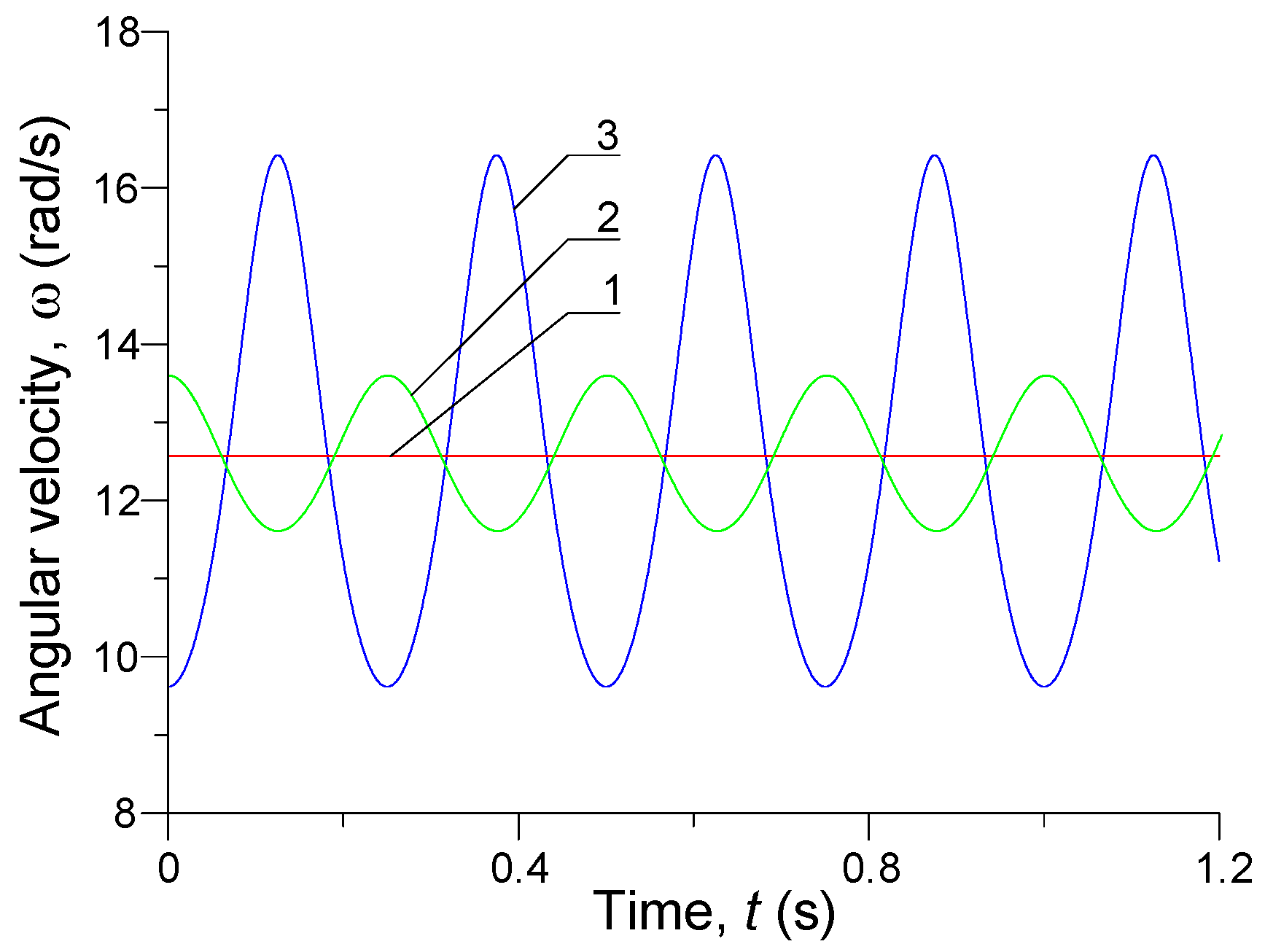
The first experiment can be treated as a demonstration. The temporal dependencies of the analysed functions are presented in the case of constant rotational speed ω_EM = 4π = const rad/s of the first shaft, assuming the absolute rigidity of the middle shaft. Figure 4 contains the temporary rotational speeds of three motion transmission shafts where the angles have the following values: α_1,2 = π/8 rad and α_2,3 = π/4 rad.

The speed of the first shaft is coloured red, that of the second (middle) is coloured green, and that of the third is coloured blue. Analysis of Figure 4 suggests that oscillatory movements with an approximate angular velocity amplitude of 17 rad/s are present in the third shaft when compared to the first. This means that mechanical corrections are necessary in precise systems with constant angles across cardan joints. Figure 4 depicts important properties of the joints: instantaneous rotational speeds at constant angles intersect at counter-phase points.

Figure 5 shows the transient angular velocity of the three motion transmission shafts where α_1,2 = π/8 sin(5t) rad and α_2,3 = π/4 sin(5t) rad have non-stationary values.

In contrast to Figure 4, both the angles between the shafts are non-stationary functions. This causes complicated motions in the system. As the functions are periodic, Fourier series can be used for their approximation. As in the previous case, angular velocity waveforms intersect at counter-phase points.

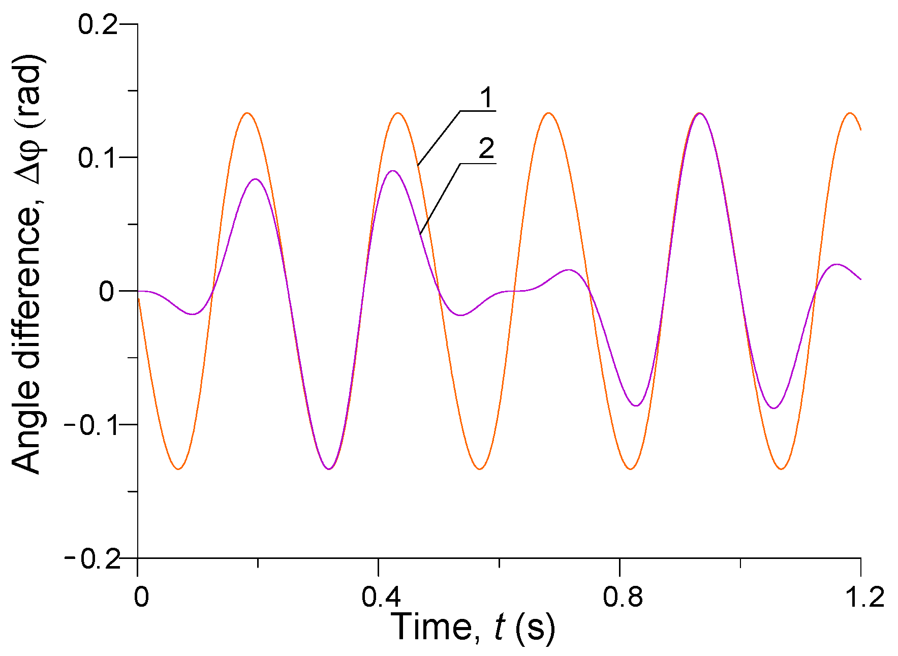
Figure 6 illustrates the rotation angle differences between the first and third shafts for the angles α_1,2 and α_2,3 constant and variable in time.

Section 2 discusses the conditions under which the rotation speeds of the first and third shafts can be identical. Equal angles between the adjacent shafts are crucial. Figure 7 shows the rotational speed waveforms of the three shafts for the angles variable in time and equal to one another, α(t)_1,2 = α(t)_2,3.

The rotational speed waveform of the second shaft is quite complicated, whereas the first and third shafts rotate at identical speeds. Such drive systems are commonly used in transport and industry.

The second experiment. The computer simulation uses an induction motor with the following rated data: P_N = 320 kW; U_N = 6 kV; I_N = 39 A; ω_N = 740 rad/s, p₀ = w, J_EM = 49 kg·m². The magnetising curve of the motor’s steel is characterised by: ψ_m = 12.4 arctg (0.066 i_m). These are the parameters of the middle shaft: G = 8.1 × 10¹⁰ Nm, ρ = 7850 kg/m³, d = 15 cm, L = 4.5 m, J_O = 50 kg·m², the loading torque is M_O = 4 kN·m, the angles between the adjacent shafts: α_1,2 = α_2,3 = π/5, α_1,2 = π/8 sin(5t), α_2,3 = π/4 sin(5t). All the functions are depicted in generalised coordinates reduced to the rotor. The non-linear system of differential equations for the system is integrated with the Runge–Kutta fourth-order method [27].

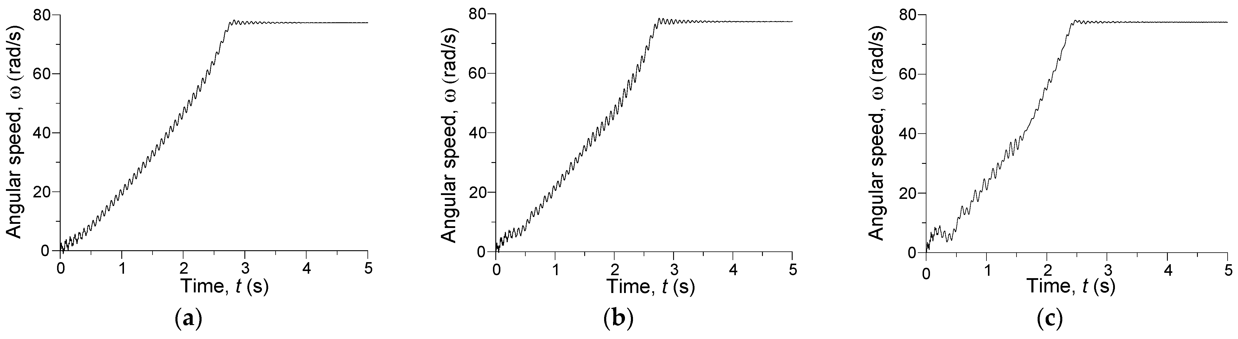
Figure 8 present instantaneous angular velocities of the drive system asynchronous rotor for the shaft diameter D = 0.1 m and three angles between the adjacent shafts: (a) α_1,2 = α_2,3 = 0, (b) α_1,2 = α_2,3 = π/8, (c) α_1,2 = α_2,3 = π/5.

A comparative analysis of Figure 8 implies the effect of angular velocity between the adjacent shafts on the drive’s start-up. Greater values of α_1,2 and α_2,3 cause additional oscillations of the rotor, which is a negative development for the motor control system.

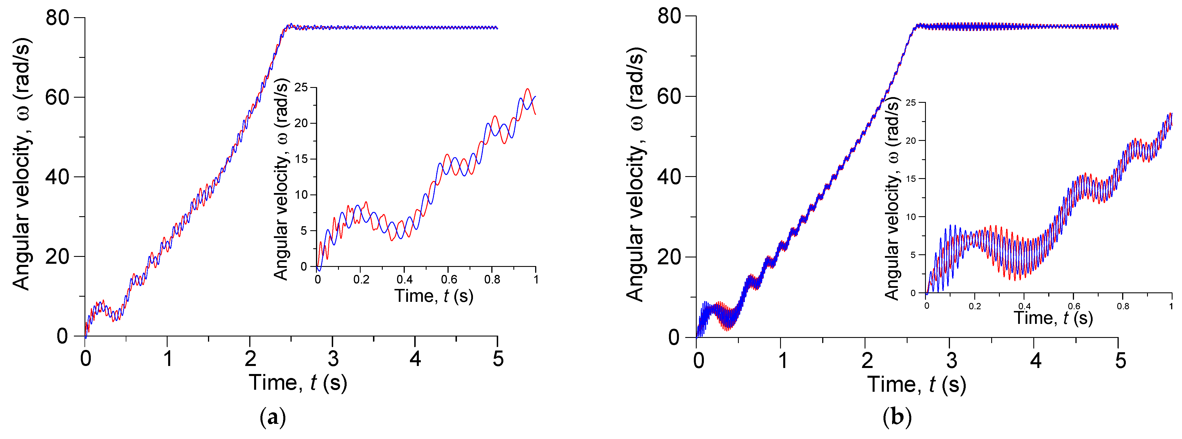
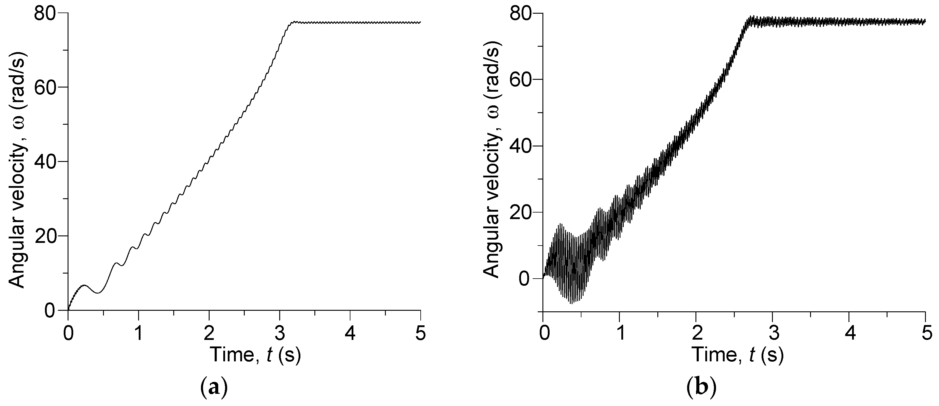
Figure 9 show transient velocities of the drive system’s asynchronous rotor and the input shaft of the loading mechanism for the shaft diameters: D = 0.1 m and D = 0.1920 m for the following angles between the adjacent shafts: α_1,2 = α_2,3 = π/5.

The system is in the operating zone prior to resonance and in a resonant state. Figure 9 illustrates angular velocity waveforms as a function of time for two shafts: the rotor of the asynchronous motor (red) and input shaft of the loading mechanism (blue) for two cases. The first case applies to D = 0.1 m—Figure 9a. The other case holds for the following parameters: D = 0.192 m—Figure 9b. Both the figures clearly show that velocities of both the shafts are identical in the steady state. In transient states, on the other hand, when oscillatory processes are present across the shaft, the velocities are different. It is clear that for the smaller shaft diameter, the velocity oscillations are in counter-phase; see Figure 9a. In Figure 9b, the system is resonant. It is impossible, as for dual-mass systems, to distinguish a priori a specific resonant frequency. The zone of resonance can be defined here.

Figure 10 depicts an instantaneous angular velocity of the rotor for identical angles between the adjacent shafts: α_1,2 = α_2,3 = π/5 and for different shaft diameters.

In Figure 10a, the shaft diameter is D = 0.3 m, while in Figure 10b, D = 0.1825 m; i.e., the system is in the resonance zone. A comparison of Figure 10 suggests a relatively large impact of resonance on the rotor’s rotational speed, which is very dangerous for the drive’s power section.

Figure 11 show instantaneous moments of torsion in the middle shaft sections for varying shaft diameters D and the angle between shaft axes α_1,2, α_2,3.

In Figure 11a, D = 0.1825 m and α_1,2 = α_2,3 = π/5. In Figure 11b, D = 0.3 m and α_1,2 = π/8 sin(5t), α_2,3 = π/4 sin(5t). The system in Figure 11a is in the resonant zone, and that in Figure 11b is out of the resonant zone. If the torque of drive loading is 4 kNm, the amplitude of moments of torsion in resonance reaches even 140 kNm—Figure 11b. Where the drive is in the steady state, on the other hand, the amplitude is approximately 14 kNm. In the resonant state, the electric drive obviously cannot operate properly.

Figure 12 depicts an instantaneous electromagnetic torque of a deep bar cage induction motor for the following shaft parameters: D = 0.3 m, α_1,2 = α_2,3 = π/5.

The speed ratio values cause electromagnetic torque oscillations not only in the transient state but also the steady state, since the drive loading torque rises periodically. Figure 12b contains graphs for two shafts: asynchronous motor rotor (red) and left end of the middle shaft (green) with the following parameters: D = 0.3 m, α_1,2 = π/8 sin(5t), α_2,3 = π/4 sin(5t). The system is in its normal operating condition, i.e., out of resonance. The time-variable cardan joint speed ratio causes an oscillatory rumble in the middle shaft. In this case, the drive motor in the steady state rotates with a constant rotational speed.

Figure 13 shows spatial–temporal waveforms of shaft angular velocity in the time range t $\in$ (0.34; 0.42) for the shaft diameter D = 0.1825 m, α_1,2(t) ≠ α_2,3(t) and rotation angle in the time range t $\in$ (0.18; 0.26) for the shaft diameter D = 0.1825 m, α_1,2 = α_2,3 = π/5.

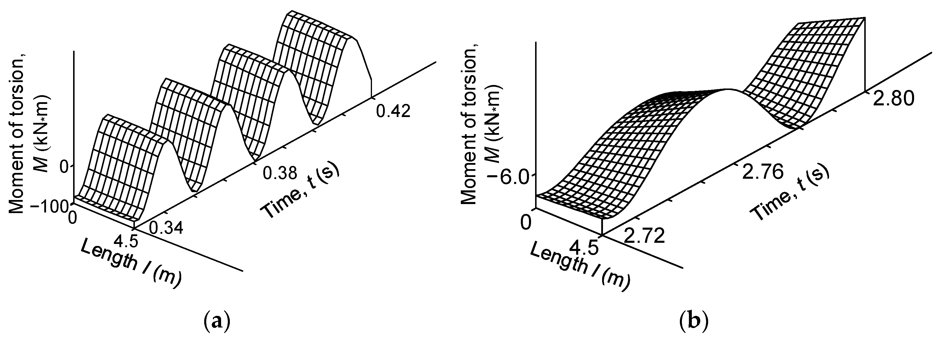
Figure 14 presents spatial–temporal waveforms of moment of torsion across the shaft.

In Figure 14a, D = 0.1825 m, α_1,2 = α_2,3 = π/5. In Figure 14b, D = 0.3 m, α_1,2 = α_2,3 = π/5. Analysis of the 3D graphs clearly shows the highly complicated processes in the middle susceptible shaft with distributed mechanical parameters. The angular velocities and rotation angles of the shaft’s spatial discretisation nodes change in line with the laws of physics. The moment of torsion as a function of the coordinate x changes according to the value of the cardan joint speed ratio. Mechanical waves in reducer-free systems are known to lead to a virtually identical moment of torsion across shafts [32,33].

Figure 15 illustrates the instantaneous ratios of the loading mechanism’s shaft rotational speed to the rotational speed of the rotor (∆) dependent on the shaft diameter for: D = 0.1 m α_1,2 = α_2,3 = π/5—Figure 15a and D = 0.3 m α_1,2 = α_2,3 = π/5—Figure 15b.

The ratio of the rotational speed of the loading mechanism’s input shaft to the rotational speed of the rotor (∆) can be treated as the total speed ratio between the rotor and the loading mechanism’s shaft. If the angles between adjacent shafts are identical, that ratio will equal one, of course for absolutely rigid shafts. If the other shaft is susceptible, the resultant speed ratio ∆ in transient states is a function of the shaft angle difference variation. Figure 15a demonstrates ∆ for a small shaft diameter and Figure 15b demonstrates ∆ for a working diameter value. In the former case, the shaft’s rigidity is low, which causes an oscillation amplitude of the resultant speed ratio. The oscillations have an amplitude approximately twice as large as in the case shown in Figure 15b. These processes evidently complicate the control of the drive systems analysed to a great degree.

Figure 16 illustrate instantaneous stator A phase currents and the rotor’s virtual A phase currents.

The theory of electric machines assumes the replacement of a multi-phase rotor cage bar system with a virtual three-phase system of generalised coordinates. Analysis of Figure 14 implies that the current waveforms are results of mechanical processes that arise from the complicated motion transmission. Thus, the oscillatory nature of the motor’s electromagnetic torque can be inferred; see (37).

The results of computer simulations certainly prove that the susceptibility in shafts of motion transmission systems including cardan joints must be addressed. In particular, the susceptibility must be taken into account in asynchronous drive systems in direct start-up as well as when reversing and braking. Start-up and moments of torsion produce highly complicated movements, as analysed in this study.

6. Conclusions

Use of the electromagnetic field theory enables describing highly complicated processes in rotor cage bars that address the skin effect. Starting from there, a mathematical model of a non-linear deep bar cage asynchronous motor is developed. The model can be used as part of a drive system with a great degree of adequacy.

The mathematical model of a three-shaft motion transmission including long shafts requires shaft susceptibility to be addressed. Therefore, the wave motion equation of the long elasticity torque is employed, which addresses the mechanical wave movement along the shaft continuum at the level of mechanical fields. This allows for considering the latent complicated motions present in the electromechanical system.

In motion transmissions of ordinary mechanisms and three-shaft drive systems, a system containing cardan joints needs ultimately to be analysed as follows: the first and third shafts as an absolutely rigid system, whereas the intermediate, second shaft as an elastic–dissipative continuum of distributed mechanical parameters.

The results of computer simulation of transient processes across a three-shaft system of susceptible motion transmission including two cardan joints suggest the following conclusions:

• Given the stationary angles between adjacent shafts, when the first rotates at a constant speed, the remaining shafts rotate according to a periodic function describing the value of the cardan joint speed ratio;
• Regardless of how angles between adjacent shafts are described, if the functions describing the values of a cardan joint speed ratio are identical in time and the three-shaft system is in a single plane of the first and third shafts’ rotation speed, the speeds of the first and third shafts are convergent, while in elastic systems, these speeds may differ;
• Addressing non-stationary angles between adjacent shafts substantially complicates transient processes in the system of susceptible motion transmission including cardan joints;
• A change of the middle shaft’s parameters in the susceptible motion transmission including cardan joints changes the range of torsional oscillation frequency, which is dangerous in such systems as it may give rise to resonant processes and vibration rumbling;
• In asynchronous drives containing susceptible motion transmission including cardan joints, the transient states of the system must be analysed including variations of the drive motion transmission parameters.