Research on Machining Workshop Batch Scheduling Incorporating the Completion Time and Non-Processing Energy Consumption Considering Product Structure

Abstract

Energy-saving scheduling is a well-known issue in the manufacturing system. The flexibility of the workshop increases the difficulty of scheduling. In the workshop schedule, considering the collaborative optimization of multi-level structure product production and energy consumption has certain practical significance. The process sequence of parts and components should be consistent with the assembly sequence. Additionally, the non-production energy consumption (NPEC) (such as the energy consumption of workpiece handling, equipment standby, and workpiece conversion) generated by the auxiliary machining operations, which make up the majority of the total energy consumption, should not be ignored. A sub-batch priority is set according to the upper and lower coupling relationship in the product structure. A bi-objective batch scheduling model that minimizes the total energy consumption and the total completion time is developed, and the multi-objective gray wolf optimizer (MOGWO) is employed as the solution to obtain the optimal schedule scheme. A case study is performed to demonstrate the potential possibilities concerning NPEC in regard to reducing the total energy consumption and to show the effectiveness of the algorithm. Compared with the traditional optimization model, the joint optimization of NPEC and PEC can reduce the energy consumption of standby and handling by 9.95% and 22.28%, respectively.

1. Introduction

Scheduling has been certified to be critical in manufacturing for improving the productivity of the manufacturing system and utilization of equipment, as well as shorting the manufacturing cycle [1]. Traditional machining scheduling typically envisions product processing phases where jobs are independent of each other and are not sequence constrained. In the conventional processing scheduling method, the two processes of processing and assembly are separated from each other, which will lead to the destruction of the original parallel relationship between processing and assembly [2]. Generating a processing sequence on the base of the assembly process would reduce the frequency of this phenomenon. Nevertheless, because the process is complicated (such as product hierarchy, number of workpieces, and processing steps), the resolution of these problems considered processing sequence in machining systems is more difficult than traditional machining scheduling. Moreover, it is an NP-hard problem [3].

Temporally, the completion time of workpieces is affected by the hierarchy of the product tree. For example, a product that includes 10 levels is processed from the bottom up. If each level is processed when the previous level is finished, without a doubt, it will prolong the entire production cycle. Therefore, batching the workpieces and making the scheduling scheme in the production of the multi-level structures have practical significance for reducing the completion time.

The manufacturing industry has consumed large amounts of energy in the process of transforming resources into products or services, leading to many environmental problems [4]. The realization of low-carbon manufacturing is extremely important for improving the sustainability of the manufacturing industry [5]. Energy-efficient scheduling, which can be approved in the manufacturing industry, has achieved energy conservation and emissions reduction [6]. Therefore, the scheduling scheme should not only consider the rationality of the process sequence for the workpieces but also reduce the energy consumption of the production system.

The processing energy consumption (PEC) and non-processing energy consumption (NPEC) of the machine are the two components of the production energy consumption of the workshop. PEC stands for the energy consumption of the machine at the processing stage, which is related to the processing power and processing time of the machine. NPEC is the sum of standby energy consumption, conversion energy consumption, and handling energy consumption. Compared with the energy consumed by the machine in other operating phases, the equipment consumes less energy when processing workpieces, especially in mass production, which generally only accounts for approximately 10% of the total energy consumption [7].

Most of the energy consumption in production is generated by auxiliary operations. Here, auxiliary operations are defined as operations that are not directly involved in processing but indispensable in the production process, such as those for equipment standby, state conversion, and workpiece handling. Compared with the energy consumption generated by the processing phase, the energy consumption generated by auxiliary operations can be large. Therefore, if the focus of energy conservation is on developments in processing and energy-saving equipment [8], the considerable energy-saving potential of auxiliary operations will be ignored. In addition, relative to changing a processing technology or researching and developing more energy-saving processing, an optimized workshop scheduling scheme can provide good application value with a low investment [9]. Therefore, in a production system based on processing sequences of workpieces, comprehensively considering the energy consumption composition in the production process, optimizing the allocation of workshop resources, and formulating reasonable scheduling arrangements will be more conducive to reducing energy consumption and improving efficiency in manufacturing enterprises.

Gray wolf optimization [10] (GWO) is a new intelligent optimization algorithm proposed in recent years. Compared with the genetic algorithm (GA) and particle swarm optimization (PSO), GWO algorithm results are more competitive [11]. At present, the gray wolf algorithm has been widely applied in thermodynamics [12], power systems [13], energy and fuels [14], cloud technology [15], and workshop scheduling [16,17,18]. Lu [16] embedded genetic operators into the multi-objective GWO to enhance the searchability of the algorithm. Qin [17] used the improved multi-objective gray wolf algorithm to solve the casting shop scheduling to minimize the production cycle, total production cost, and total delivery delay. Lu [18] added a random search model based on traditional GWO search to enhance global search capability. Although GWO has been successfully used in many different types of production environments, there is limited literature on GWO to solve energy-saving scheduling problems in a machine-shop, especially to optimize auxiliary production energy consumption. Therefore, we extended the single-objective GWO to the multi-objective GWO to consider completion time and total energy consumption minimization.

Reducing energy consumption through NPCE optimization and minimum completion time are major design goals. The research motivation and research problem will be clearer in the discussion of background research, and then the related mathematical model will be introduced, followed by the MOGWO algorithm and how it is applied to optimize the bi-objective scheduling problem; finally, a presentation of a case study will demonstrate the model and algorithm in the case of two different energy consumption optimization objectives and different algorithms.

In the rest of this paper, the current research progress will be introduced in Section 2 and a bi-objective model based on the research problem is established in Section 3. In Section 4, the working procedure of MOGWO of this optimization problem is described. Section 5 conducts case analysis and comparison. Finally, Section 6 summarizes this article.

2. Literature Review

The scheduling research of multi-level structure products was first studied for an assembly workshop [19,20]. Li et al. [21] developed four batch strategies to solve three different multi-level product assembly problems. Lu et al. [22] studied tree-like products scheduling problems in an assembly workshop, aiming to minimize the assembly completion time. Wan et al. [23] proposed a visual modeling and scheduling model for assembly processing based on a workflow for the assembly process of complex products and designed heuristic scheduling rules. Suharyanti et al. [24] investigated the optimal lot size of complex products in the job shop. Batching can effectively reduce product production cycles. However, the scheduling research on multi-level structure products is not enough to solve the problem of collaboration production because sequence constraint scheduling should be compatible with the assembly sequence and has higher complexity.

A scheduling problem that comprehensively considers the optimization of the energy consumption with the traditional targets (completion time/production cost) is complex, and it is particularly important to carry out in-depth research on this [25]. At present, a large amount of energy waste occurring in processes that have nothing to do with equipment processing operations has been found. Dahmus and Gutowski [7] analyzed the energy consumption of machining and proved that the actual processing operations only accounted for a small part of the total energy consumption, whereas auxiliary operation energy consumption accounted for 30–50%. The idle time of the machine occupied 16% of the total completion time [26]. Thus, the NPEC is large. Based on the knowledge regarding total energy consumption, it has become a trend to decompose the total energy consumption and reduce energy waste through optimization of the scheduling scheme. Wang [27] simulated a processing process and classification of energy consumption by product quality. In general, the total energy consumption can divide into PEC and NPEC, where NPEC, as indicated above, refers to the energy consumption generated by auxiliary operations such as equipment start-up, shutdown, and idling.

In recent years, more and more research of NPEC has been conducted thoroughly. Luan et al. [28] studied the energy consumption of non-cutting status and established an accurate power model to accurately predict the power of the feed motion. Liu et al. [29] improved the machine utilization rate by 8.2% by optimizing the processing sequence for the workpieces. Peng et al. [30] considered standby energy consumption. Wu et al. [31] studied a renewable energy scheduling problem of a flow shop and established a multi-objective renewable energy power supply model, intending to reduce the processing and idle energy consumption during processing. Gilles et al. [32] investigated the impacts of batch production on energy consumption and order completion time. It was considered that batching could effectively reduce the number of conversions and equipment standby time, thereby reducing the conversion energy consumption and standby energy consumption. Che et al. [25] used a clustering algorithm to determine whether a shutdown operation was required between two tasks to reduce the standby energy consumption and/or optimally sort the processing tasks. Liu et al. [29] integrated scattered short standby periods into a long standby time and judged whether off or assigned other tasks. Wang et al. [33] considered the power changes in the standby state and processing states of the machine. However, the above research mostly focused on the conversion and standby energy consumption separately. In the research of NPEC, they should be considered more systematically.

In the research articles above, most of the influences of workpiece handling on the energy consumption of the workshop were ignored. However, it is more realistic to consider the scheduling and optimization of such handling. The impact of handling on energy consumption has generally not been considered [34,35,36]. The handling of workpieces between machines is also part of auxiliary processing, and its energy consumption should belong to the NPEC in the system. Different from previous studies, the NPEC would be determined based on the energy consumption of the equipment standby, conversion, and workpiece handling. In addition, a machine may perform many processing tasks, and the frequent shutdown and start-up of the equipment will increase energy consumption. Therefore, this part of the energy consumption is generally not considered.

Based on the above discussion, the research on multi-level product production and energy-conscious scheduling in the machining workshop is limited. The existing workshop scheduling methods cannot meet the requirements of production and energy saving because each mode has its characteristics. The research on NPEC should be considered when proposing a scheduling method that is different from the traditional optimal energy consumption scheduling. Therefore, the scheduling model of the machining workshop is more complicated than that of the traditional workshop. To bridge this gap, a scheduling method was introduced specifically for machining workshops to minimize completion time and energy consumption.

3. Problem Statement

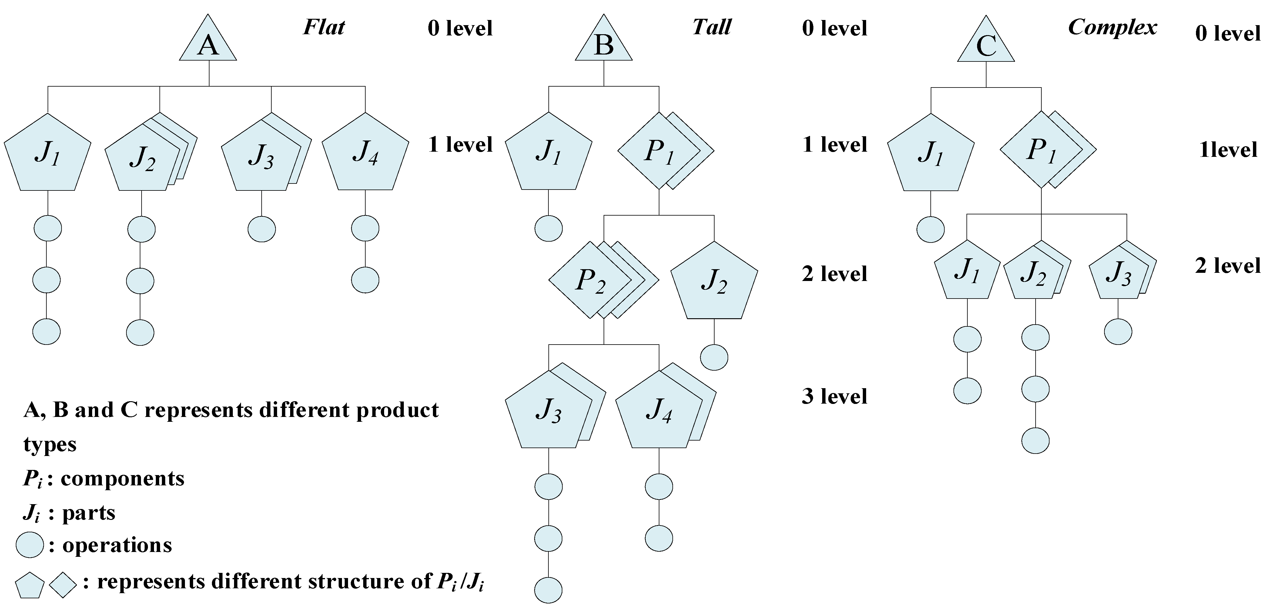
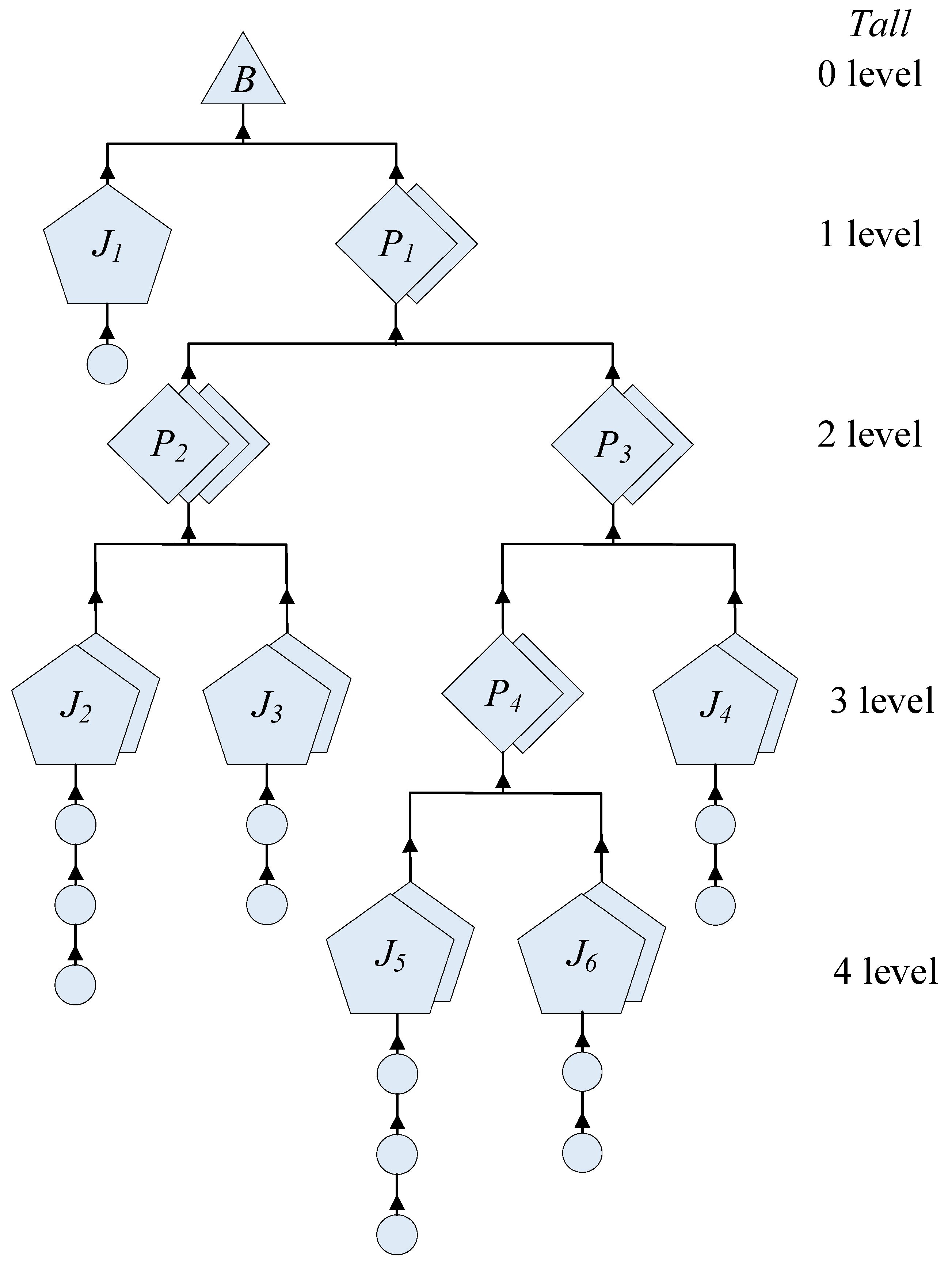
3.1. Related Product Structure

In real-world production, a product is a combination of a group of parts/components with order constraints and can be represented using a tree structure diagram. The processing and assembly of products are conducted according to the tree structure. The edges in the tree represent the assembly constraint relationships, the leaf nodes are the parts/components, and the root node is the final product. Each level’s leaf node can be called a child node of its upper-level node, and the processing starts from the lowest-level leaf node. It is composed of n parts/components with order constraints. The production of components includes several processes, each process is handled by a machine (in M), and the alternative processing equipment for different processes can be identical.

According to the structural characteristics and commonalities between products, the literature [37] has generally summarized product structures into three types: flat, tall, and complex. The corresponding product structure trees are shown in Figure 1. The flat type is a single-layer product and is directly assembled from first-level parts into products. The tall type has multiple levels of parts/components, and each sub-workpiece contains at most two nodes. The complex type is a multi-layer composite of flat- and tall-type tree structures, in which at least one parent node contains more than two child nodes, as shown in Figure 1. The nodes of each tree are arranged hierarchically, where level 0 represents the complete product, and level 1 is the hierarchical arrangement of parts. For example, the structure of the B product is divided into 1–3 levels, and the branch nodes under it are called components, such as P₁ and P₂. The production sequence is as follows: first produce the workpieces J₃ and J₄, and then the superior P₂ and J₂ for production, and so on.

Based on the coupling relationship(s) between the parts/components in the product structure, batch production and handling are conducted, in which each type of workpiece is divided into equal batches, and the numbers and size of the sub-batch of each product are determined, as well as the sub-batch production and handling sequence. A batch scheduling problem based on the product structure will face difficulties caused by the coordination of the processing times between the workpieces. The arrangement of the production sequence of each sub-batch to meet the coupling sequence of the products is very important. For example, in the mass production of the workpieces in a machining workshop, each type of workpiece can be divided into an equal number of sub-batches. According to the coupling relationship between the workpieces and the production time of the workpiece, the lower-level workpieces are produced first, and then the start processing time of the upper-level workpieces will be later than the next level of workpieces, minimizing machine standby while optimizing handling equipment to reduce NPEC.

3.2. Problem Definition and Assumptions

The problem can be expressed as follows. Related sets and decision variables are shown in the Appendix A.

• The product contains n types of workpieces J = {J₁, J₂, J₃... J_n}, the number of workpieces J_j is Q_j, and each workpiece contains O_j processes.
• There are h types of handling equipment in the workshop. A specific piece of handling equipment is expressed as H_h. The handling speed and power of the same type of handling equipment are the same; the speed of H_h is V_h, the power when handling parts/components j is $P_j^h$, and the rated capacity of the workpiece j on the handling equipment is S_jh.
• After a certain process of the workpiece is processed on equipment m, it needs to be transported to the selected equipment m’ of the next process. The locations of all equipment in the workshop are fixed, and the distance between equipment m and equipment m’ is d_mm’. After the last process of a batch of workpieces is processed on equipment m, they are transported to assembly workshop P for assembly. The distance between equipment m and assembly workshop P is d_mp.

The following assumptions are used in the scheduling.

• Alternating machines for different processes can be the same.
• Each type of sub-batch of workpieces can only be transported to the next process processing equipment for processing/waiting after the previous process is completed according to the process sequence.
• At most, one workpiece is processed on each machine at a time, and one workpiece is processed on at most one piece of equipment at any time.
• The processing and handling equipment are available at the initial moment.
• A process is not interrupted once it starts processing.
• The equipment requires preparation time before processing different types of workpieces successively; in contrast, processing the same types of parts does not require preparation time.
• The number of pieces of handling equipment is limited. If the number of sub-batches of workpieces is greater than the rated capacity of the handling equipment, multiple pieces of equipment must be moved simultaneously or multiple times by one piece of equipment.
• The time required for loading and unloading workpieces is ignored.

3.3. Problem Formulation

3.3.1. Objectives

During workpieces processing, there are three main states of equipment: the processing state, conversion state, and standby state. The equipment power and state vary with time [25], as shown in Figure 2. $S_m^i$ and $C_m^i$ represent the start and completion times of the ith operation on device m, respectively, and $O_{j^{\left(1\right)}{i}^{\left(1\right)}}^m$ represents the O_ji processing on equipment m.

The total energy consumption of the production system is composed of the PEC (E_p) and NPEC (E_n) during the processing of components and parts. Of these, the NPEC consists of the state transition energy consumption (E_s), the standby energy consumption (E_w), and the handing energy consumption (E_d) (including the energy consumption of the moving parts/components between machines and moving to the assembly workshop when finished).

• The energy consumption criterion E

It consists of the PEC and NPEC. Specifically, this energy consumption metric is given as follows:

E = E_p + E_n

(1)

The PEC consumed by all workpieces owing to the processing, as shown in Equation (2), as follows

$$E_p={{\displaystyle \sum }}_{j=1}^n{{\displaystyle \sum }}_{k=1}^{B_j}{{\displaystyle \sum }}_{i=1}^{O_j}{{\displaystyle \sum }}_{m=1}^w{\alpha }_j{\mathit{TB}}_{\mathit{jkim}}$$

(2)

The NPEC consists of the equipment standby energy consumption (E_w), conversion energy consumption (E_s), and handling energy consumption (E_d). The equation is given by Equation (3), as follows:

$$E_{n }{=E}_w{+E}_S{+E}_d$$

(3)

Among them, E_w refers to the idling state where the equipment is on non-stop, and no parts/components are processing on the machine. The formula for the energy consumption during the standby period is shown as follows:

$$E_w={{\displaystyle \sum }}_{k=1}^{B_j}{{\displaystyle \sum }}_{j=1}^n{{\displaystyle \sum }}_{m=1}^w{(\mathit{SB}}_{j(k+1)\mathit{im}}-{\mathit{CB}}_{\mathit{jkim}})P_m^w)$$

(4)

In the above, ${\mathit{SB}}_{j\left(k+1\right)m}$ represents the start time of the (k + 1)th sub-batch of j on the processing equipment m, represents the kth sub-batch on equipment m completion time, and $P_m^w$ is the standby power of the machine.

E_s represents the energy consumption of the equipment state transition. In Equation (5), $|{\alpha }_j-{\alpha }_j\prime |$ is the absolute value of the difference in energy consumption involved in switching power owing to processing different types of workpieces (j→j′); $R_{{\mathit{jj}}^{\prime }m}$ is a 0–1 variable. If the processing of the workpiece on equipment m is different from the workpieces to be processed, $R_{{\mathit{jj}}^{\prime }m}$ = 1; otherwise, $R_{{\mathit{jj}}^{\prime }m}$ = 0.

$$E_s={{\displaystyle \sum }}_{j=1}^n{{\displaystyle \sum }}_{k=1}^{B_j}{{\displaystyle \sum }}_{i=1}^{O_j}{{\displaystyle \sum }}_{m=1}^M{R}_{\mathit{jkim}}{R}_{\mathit{jj}}{\prime }_m|{\alpha }_j-{\alpha }_j\prime |$$

(5)

The workshop handling energy consumption is related to the sub-batch quantity B_pj and sub-batch Q_pjk of j, selected handling equipment H_h, distance d_mm′ between the equipment, and distance d_mP between the equipment and assembly workshop P. E_d represents the energy consumption during handling. The transportation of workpieces includes two parts: one part comprises transporting the current sub-batch process to the next processing machine after the completion of the current sub-batch process, and the other comprises transporting it to assembly workshop P after the last process of the sub-batch process is completed. The two parts of energy consumption are described in detail as follows. This can be expressed using Equation (6).

$$E_d=E_{jkim{m}^{\prime }}^h+E_{jkmP}^h$$

(6)

After the process O_ji is processed on equipment m, the workpiece will be transported to the next process O_j(i+1). The energy consumption $E_{jkim{m}^{\prime }}^h$ of the transportation equipment H_h at the selected equipment m′ is shown in Equation (7).

$$E_{jkim{m}^{\prime }}^h={\sum }_{j=1}^n{\sum }_{k=1}^{B_j}{\sum }_{i=1}^{O_j}{\sum }_{m=1}^w{\sum }_{h=1}^H{S}_{jkih}^1{H}_{jkimh}^1{n}_{jk}{P}_j^h{t}_{jkim{m}^{\prime }}^h={\sum }_{j=1}^n{\sum }_{k=1}^{B_j}{\sum }_{i=1}^{O_j}{\sum }_{m=1}^w{\sum }_{h=1}^H{S}_{jkih}^1{H}_{jiamh}^1\lceil \frac{Q_{pjk}}{s_{jh}}\rceil P_j^h\frac{d_{m{m}^{\prime }}}{V_h}$$

(7)

Here, n_jk represents the number of pieces of handling equipment required for the kth sub-batch of j, and $t_{jkimm\prime }^h$ indicates the time that H_h moves j from process O_ji of equipment m to m’. $S_{\mathit{jkih}}^{\beta }$ is a 0–1 variable. If H_h was selected to handle the ith process of the kth sub-batch of j, then $S_{\mathit{jkih}}^{\beta }$ = 1; otherwise, $S_{\mathit{jkih}}^{\beta }$ = 0. $H_{jkimh}^{\beta }$ is also a 0–1 variable. β can take two values, 1 and 2; β = 1 indicates that the workpieces are transported between equipment; β = 2 indicates that the workpieces are transported from the last piece of equipment m to assembly shop P. If the ith process of the kth sub-batch of j is transported by H_h, then $H_{jkimh}^{\beta }$ = 1; otherwise, $H_{jkimh}^{\beta }$ = 0.

After the workpieces j are processed, they are transported from equipment m to assembly workshop P by H_h. The energy consumption $E_{\mathit{jkmP}}^h$ of Hh is given by Equation (8), as follows:

$$E_{jkmP}^h={{\displaystyle \sum }}_{j=1}^n{{\displaystyle \sum }}_{k=1}^{B_j}{{\displaystyle \sum }}_{h=1}^H{X}_{jk{O}_{j}m}{S}_{jkh}^2{H}_{j\mathit{kimh}}^2{n}_{jk}{P}_j^h{t}_{jkmP}^h={{\displaystyle \sum }}_{j=1}^n{{\displaystyle \sum }}_{k=1}^{B_j}{{\displaystyle \sum }}_{h=1}^H{X}_{jk{O}_{j}m}{S}_{jkh}^2{H}_{\mathit{jlimh}}^2\lceil \frac{Q_{pjk}}{S_{jh}}\rceil P_j^h\frac{d_{mP}}{V_h}$$

(8)

In the above, $t_{jkmP}^h$ represents the time taken by H_h to transport the kth sub-batch of j from m where the last process is located to the assembly workshop P. $X_{{\mathit{jkO}}_{j}m}$ is a 0–1 variable. If the last process of the kth sub-batch of j is completed on equipment m, then $X_{{\mathit{jkO}}_{j}m}$ = 1; otherwise, $X_{{\mathit{jkO}}_{j}m}$ = 0.

• The makespan criterion C

The makespan criterion is defined as the maximum time for the last sub-batch for the equipment in the workshop to be processed and transported to the assembly workshop; ${\mathit{CB}}_{{\mathit{jB}}_j{O}_{j}m}$ represents the completion time of the last process O_j of the last sub-batch B_j of the workpiece j on the equipment m. In addition, $X_{{\mathit{jkO}}_{j}m}{S}_{{\mathit{jB}}_j{O}_{j}h}^{2l}{H}_{{\mathit{jB}}_j{O}_{j}h}^2$ represents the completion of the processing of the part j after choosing the handling equipment h and transporting it to the assembly workshop. The calculation is shown in Equation (9), as follows.

$$C={{\displaystyle \sum }}_{j=1}^n{{\displaystyle \sum }}_{m=1}^M{\mathit{CB}}_{{\mathit{jB}}_j{O}_{j}m}+{{\displaystyle \sum }}_{j=1}^n{{\displaystyle \sum }}_{m=1}^M{{\displaystyle \sum }}_{h=1}^H{X}_{{\mathit{jkO}}_{j}m}{S}_{{\mathit{jB}}_j{O}_{j}h}^2{H}_{{\mathit{jB}}_j{O}_{j}h}^2\frac{d_{\mathit{mP}}}{V_h}$$

(9)

The multi-objective model is shown in Equations (10) and (11).

f₁ = min C_max

(10)

f₂ = min E

(11)

3.3.2. Constraints

Two issues should be considered in the scheduling:

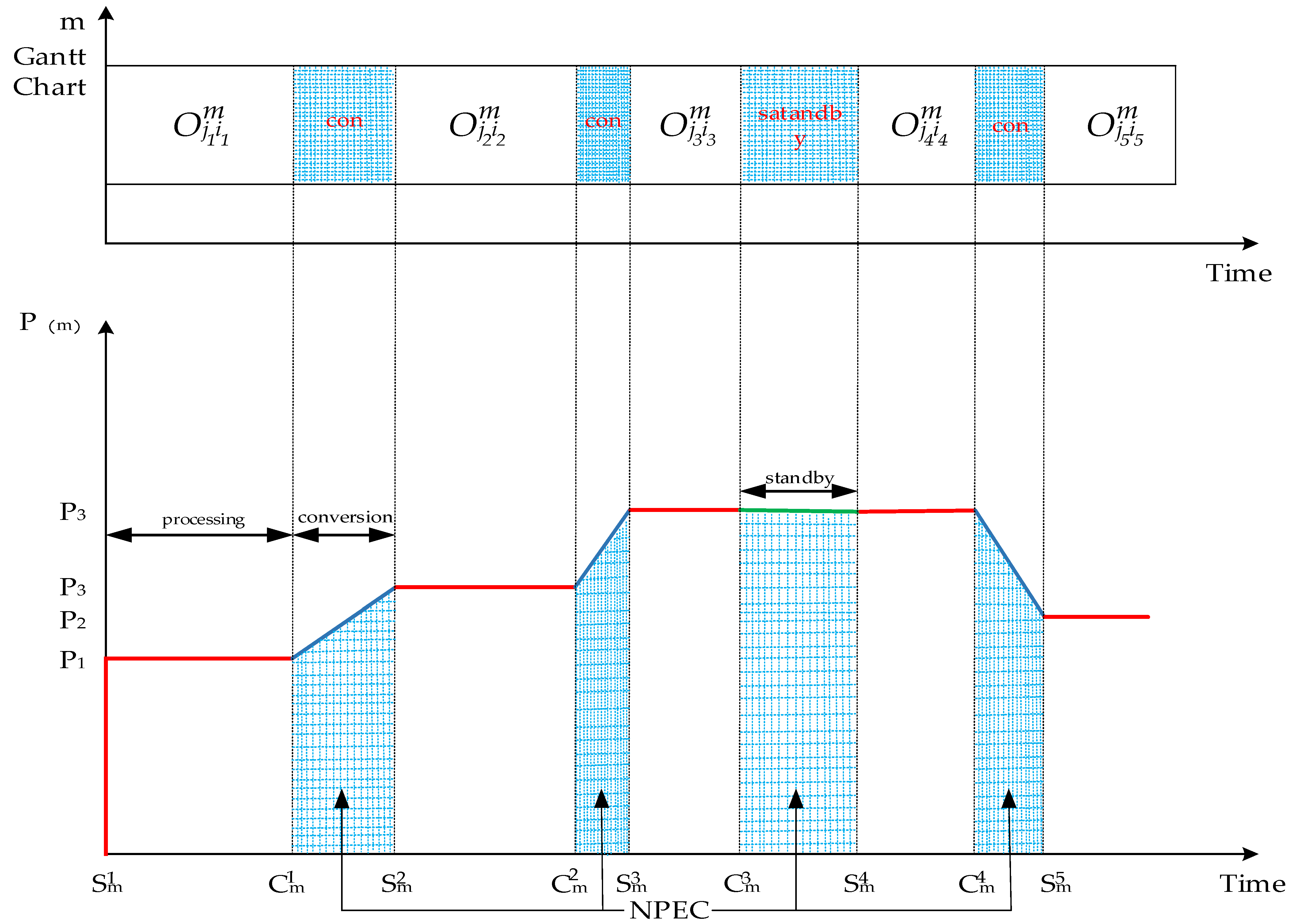
• The influences of the division of the workpieces into sub-batches, process equipment selection, equipment standby, and state transition in the processing process on the energy consumption and completion time must be considered.
• The number of handling equipment types is limited, and a type of handling equipment needs to be selected during the handling process. If a sub-batch of workpieces is larger than the rated capacity of the handling equipment, multiple pieces of handling equipment must be selected for simultaneous or multiple handling.

The batches of workpieces should satisfy the condition that the sum of the divided sub-batch batches is equal to the processing quantity of the workpieces; moreover, the number of divided sub-batches should not exceed the total quantity of workpieces.

$$\{\begin{array}{c}{Q}_j={\displaystyle \sum _{k=1}^{B_j}}{Q}_{\mathit{jk}}\\ 2\le B_j\le Q_{\mathit{jk}}\end{array}$$

(12)

The workpieces are split into equal batches. If the number of batches is not an integer, it is rounded down, and the remaining workpieces comprise a single batch.

$$Q_{\mathit{jk}}=\{\begin{array}{c}\lfloor Q_j{÷B}_j\rfloor k\le B_{j-1}\\ Q_j{-\lfloor Q}_j{÷B}_j\rfloor {\times (B}_j{-1) k=B}_j\end{array}$$

(13)

If the processing type of the current workpieces is the same as that of the workpieces being processed, there is no need to switch the state of the machine; otherwise, the state needs to be switched.

$$R_{j{j}^{\prime }m}=\{\begin{array}{l}0,P_{j\prime k\prime i\prime m}=N{P}_{jkim}\\ 1,P_{j\prime k\prime i\prime m}\ne N{P}_{jkim}\end{array}$$

(14)

The scheduling is performed according to the sub-batch priority relationships of the parts/components in the product structure tree. The process starts processing time at the completion time of the last sub-batch process in the selected equipment, and the sub-batch workpieces after the previous process are completed and transported according to the maximum value between the device moments.

$$\{\begin{array}{c}{\mathit{SB}}_{{\mathit{jkO}}_{j1}m}{=\mathit{CB}}_{{\mathit{jko}}_{j}m}=0 \\ {\mathit{SB}}_{\mathit{jkim}}{=\mathit{max}\{\mathit{CB}}_m^{n-1}{,\mathit{CB}}_{\mathit{jk}\left(i-1\right)m^{\prime }}{+t}_{{\mathit{jkimm}}^{\prime }}^h\}\end{array}$$

(15)

The production process of the same sub-batch should not be interrupted.

$${\mathit{CB}}_{\mathit{jkim}}{=\mathit{SB}}_{\mathit{jkim}}{+\mathit{TB}}_{\mathit{jkim}}$$

(16)

The part production sequence should meet the requirement that the production time of the lower-level parts/components is earlier than the start-up time of the upper-level parts/components; that is, the start-up time of the first process in the n-level parts/components sub-batch should be later than the (n + 1) level parts/components.

$$S_{\mathit{jn}1} \ge { S}_{j\left(n+1\right)1}$$

(17)

Among them, S_jn1 is the start time of the first process of the n-level parts/components, and S_j(n+1)1 is the start time of the first process of the first sub-batch of the (n + 1) parts/components j.

For two adjacent processes for the same workpiece, the processing sequence constraints between the processes need to be met, and the next process can only be conducted after the previous process is completed and the workpiece is transported to the selected equipment m′ for the start of the next process.

$${\mathit{SB}}_{{\mathit{jk}(i+1)m}^{\prime }}\ge R_{{\mathit{jj}}^{\prime }m}{R}_{\mathit{jkim} }{+\mathit{TB}}_{{\mathit{pjko}}_{\mathit{ji}}}{+t}_{\mathit{jkimm}\prime }^h$$

(18)

In each process, O_ji can only select one piece of machine for processing.

$${\displaystyle \sum }_{m=1}^w{\mathit{MP}}_{\mathit{jim}}=1$$

(19)

One type of handling equipment is selected for each handling instance.

$${\displaystyle \sum }_{h=1}^H{H}_{\mathit{jkimh}}^{\mathsf{\beta }}=1$$

(20)

4. Multi-Objective Gray Wolf Optimization Algorithm

4.1. Basic Gray Wolf Optimization Algorithm

Mirjalili [10] proposed the gray wolf optimizer (GWO) in 2014. The core of the algorithm is to manage an optimization problem by imitating the hunting process of a gray wolf population. Owing to its balance of local and global search capabilities, convergence speed, and depth balancing, it has attracted widespread attention since its proposal.

The basic idea is that α wolf was chosen to be the most suitable plan, and β wolf and δ wolf were the second and third optimal plans. The rest are ω. α and β are the guiders of hunting, followed by δ and ω wolf. The equation for simulating the corresponding behaviors is defined as follows.

$$\overrightarrow{D}=\left|\overrightarrow{C}\cdot \overrightarrow{X_p}(t)-\overrightarrow{X}(t)\right|$$

(21)

Among them, $\overrightarrow{D}$ represents the distance to the prey, t indicates the current iteration, $\overrightarrow{X_p}$ represents the prey’s position vector, and $\overrightarrow{X}$ represents the wolf’s position vector. The coefficient vectors are represented by $\overrightarrow{A}$ and $\overrightarrow{C}$, and the formula is:

$$\overrightarrow{A}=2\overrightarrow{a}\cdot \overrightarrow{r_1}-\overrightarrow{a}$$

(22)

$$\overrightarrow{C}=2\overrightarrow{r_2}$$

(23)

In the search process, $\overrightarrow{a}$ linearly decreases from 2 to 0 and is used to emphasize detection and discovery of prey. $\overrightarrow{R_1}$ and $\overrightarrow{r_2}$ are selected in the range [0,1] randomly. α, β are the guider in hunting, and δ wolves also can join the hunting. The location of the prey (optimal) is unknown. Simulating the hunting behavior of gray wolves, α, β, and δ wolves are assumed to be more familiar with the potential location of their prey. In each hunt for prey, the three best solutions represented by α, β and δ wolves will be saved and used in each search, guiding other wolves to the possible position of the prey. The hunting formula is given by Equations (24)–(26).

$$\overrightarrow{D_{\alpha }}=\left|\overrightarrow{C_1}\cdot \overrightarrow{X_{\alpha }}-\overrightarrow{X}\right|,\overrightarrow{D_{\beta }}=\left|\overrightarrow{C_2}\cdot \overrightarrow{X_{\beta }}-\overrightarrow{X}\right|,\overrightarrow{D_{\alpha }}=\left|\overrightarrow{C_1}\cdot \overrightarrow{X_{\alpha }}-\overrightarrow{X}\right|$$

(24)

$$\overrightarrow{X_1}=\overrightarrow{{ X}_{\alpha }}-\overrightarrow{A_1}\cdot \overrightarrow{D_{\alpha }},\overrightarrow{X_2}=\overrightarrow{X_{\beta }}-\overrightarrow{A_2}\cdot \overrightarrow{D_{\beta }},\overrightarrow{X_3}=\overrightarrow{{ X}_{\delta }}-\overrightarrow{A_3}\cdot \overrightarrow{D_{\delta }}$$

(25)

$$\overrightarrow{X}(t+1)=\frac{\overrightarrow{X_1}+\overrightarrow{X_2}+\overrightarrow{X_3}}{3}$$

(26)

All in all, GWO starts with guiding the search process by α, β, and δ. When $\left|\overrightarrow{A}\right|$> 1, they diverge and look for prey; otherwise, they find and attack the prey. Finally, if the stopping criterion is met, the optimal solution (i.e., prey) is output. In brief, in each iteration of the algorithm, individuals in the population were divided into α, β, δ and ω. The first three belong to the individuals at the decision-making level, representing the historical solution of optimal, suboptimal, and third optimal. ω corresponds to the other individuals. In the algorithm iterations, α, β and δ are locating prey and guiding ω to update its position, completing a sequence of actions including approaching, surrounding, and attacking the prey.

4.2. Application of Multi-Objective Gray Wolf Algorithm

The multi-objective gray wolf algorithm (MOGWO) [38] added two new components based on the gray wolf algorithm by Mirjalili in 2016. The first component is the archive, which served to store the currently acquired non-dominant Pareto optimal solutions. Then comes the leader selection strategy, which helps decision-makers to choose α, β and δ as the leader of the search process from the archived results. The basic flow chart is shown in Figure 3.

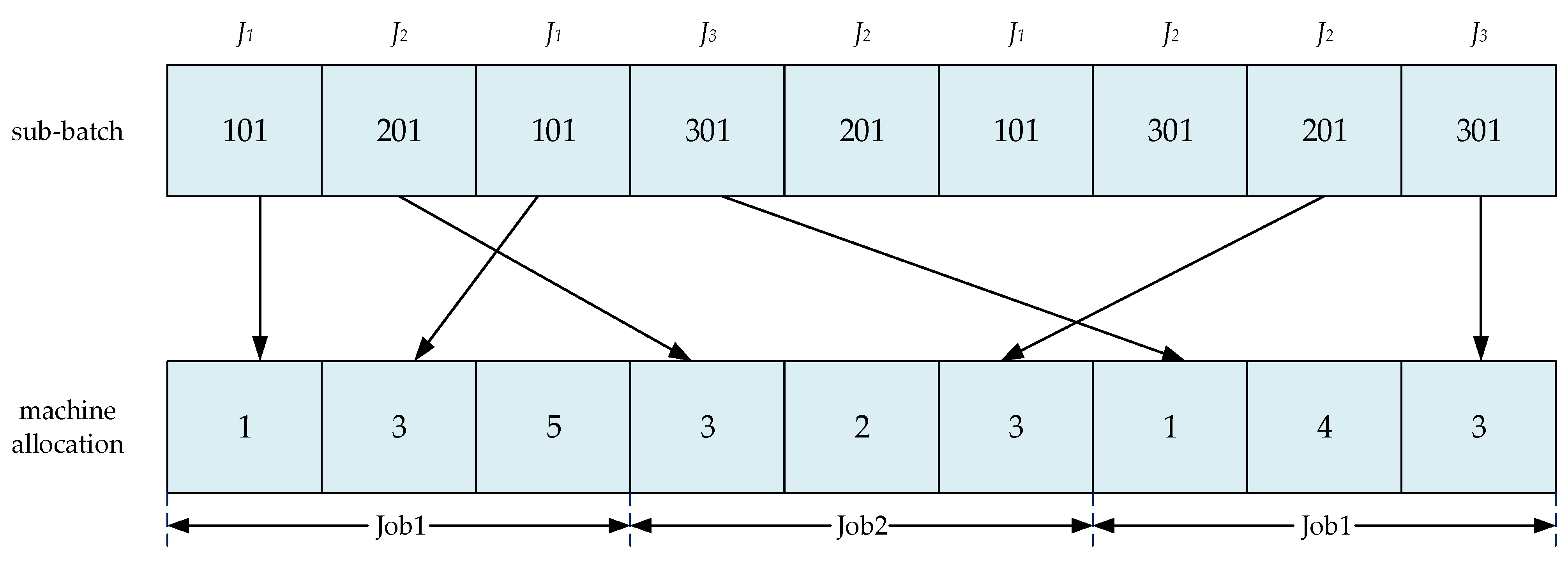
4.2.1. Encoding and Decoding Mechanism

Before applying the MOGWO algorithm to a specific problem, we designed an encoding and decoding scheme. It connects the solution space of the problem with the search space under consideration. Hence, designing the correct codec scheme is an important issue that affects the performance of the algorithm.

Code design is based on the types of parts/components and the number of batches. In each chromosome, a gene is represented by three or four numbers. For example, “301” represents the first sub-batch of the third parts/components, and “1003” represents the third sub-batch of the tenth parts/components. In addition, the number sequence in the chromosome represents the processing operations of each sub-batch of parts/components. As shown in Figure 4, each type of part/component needs to go through multiple processing operations. The first occurrence of “101” represents the first processing operation of the first sub-batch of parts/components J₁, and the second occurrence represents the second processing operation, and so on. Taking an example for illustration, the optional processing equipment of three types of workpieces and the processing time for each process are shown in

Table 1. Equipment scheduling problem, for example (unit: min).

Sub-Batch	Quantity	Operations	M1	M2	M3	M4	M5
101	30	O11	2	-	5	-	6
		O12	-	6	5	6	-
		O13	4	3	-	-	8
201	40	O21	5	-	4	-	-
		O22	9	5	-	6	-
		O23	-	5	4	7	-
301	30	O31	6	-	9	10	-
		O32	5	7	-	6	-
		O33	-	8	6	-	7

.

According to the coding method of the part/component arrangement, it can be assumed that the position of a gray wolf individual in this problem is [1,2,3], that is, the processing order of the parts/components is 1-3-2. Then, the part/component placement is decoded into a viable scheduling scheme. A Gantt chart corresponding to the first sub-batch of parts/components is shown in Figure 5. Through the decoding process, a suitable machine is selected for each process in each station for processing, and the order of each part and the start time are determined to obtain the objective function value. In Figure 5, initially, all the processes of the first sub-batch of J₁ are arranged on the machine that can process it earliest, and then the other sub-batches of other parts/components are scheduled. The various processes of the parts/components are arranged on the machine that can complete its processing earliest; if the processing completion time on the allocated machine is less than the earliest processing start time of the scheduled parts/components, it will be arranged before the scheduled parts/components (and so on for the remaining parts/components). Each sub-batch of parts is arranged before the position of each machine; otherwise, it is arranged behind the arranged parts/components.

4.2.2. Initialization

Initial solutions can affect the obtaining of the optimal solution to a degree. In our study, the problem can be divided into two sub-problems: equipment selection and process sequencing. Therefore, in the initialization phase, the most suitable processing equipment with the lowest processing energy consumption and processing time is selected based on the above encoding and decoding scheme. Then, the sorting plan is obtained according to the processing priority rules of the workpiece and the remaining load at most.

4.2.3. Roulette Selection

In a multi-object search space, comparing solutions is usually not easy; thus, the leader selection mechanism has been designed to solve this problem. The leader provides the α, β, and δ wolves in the least crowded search places. The selection is performed by using the roulette method. The probability of each hypercube is calculated as follows: two individuals are randomly selected from N individuals each time, and the individuals with the lower ranking levels are selected first. If the ranking levels are the same, the crowding degree is the first large individual to generate a population of N/2 individuals. The process merges the two generated populations into a new progeny population (population size is N).

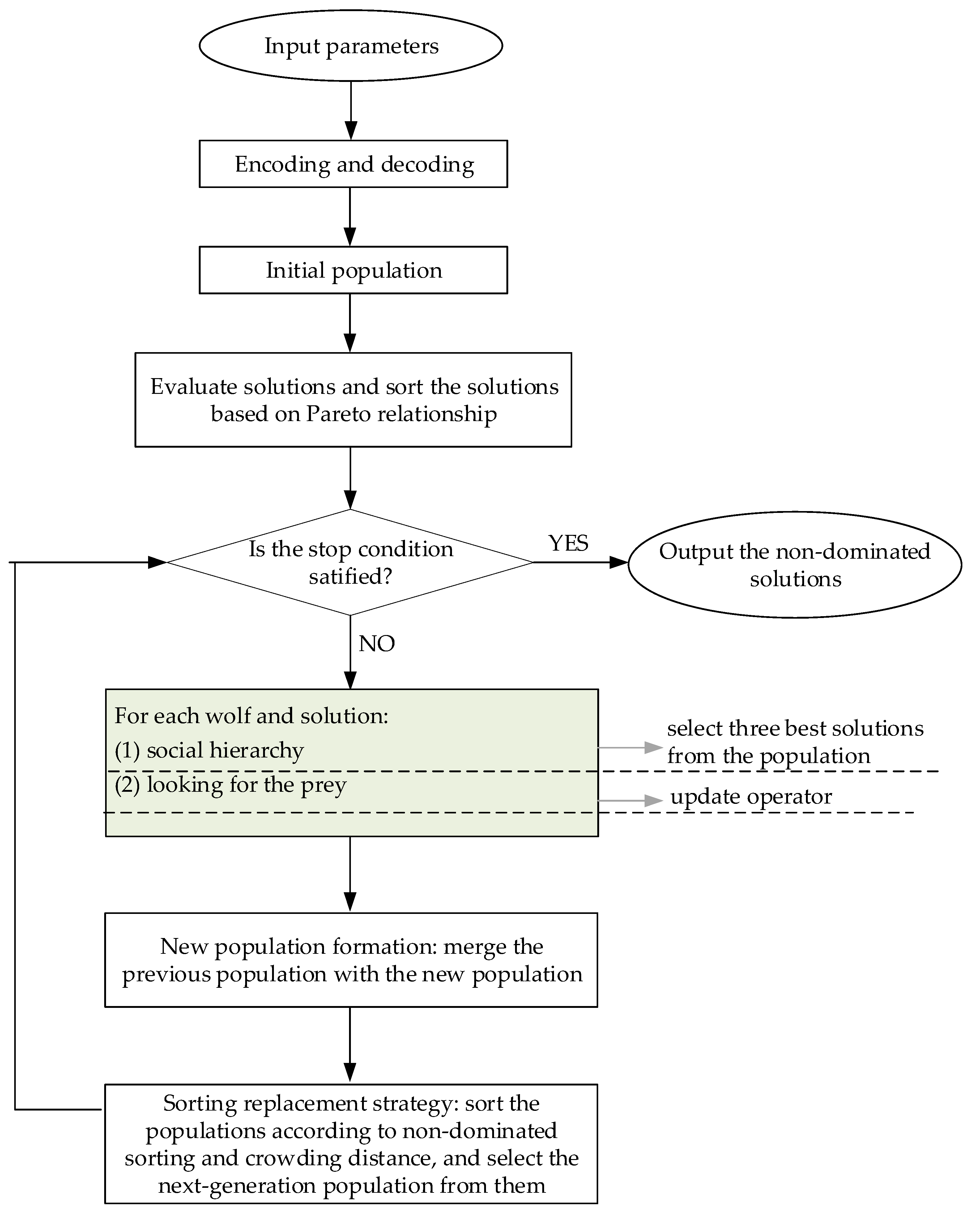
4.2.4. Social Hierarchy

Due to the Pareto advantage of multi-objective planning, the optimal result is usually not a single, which is called a “trade-off solution” in multi-objective planning. According to the Pareto dominance relationship, a population can be divided into several levels. The first-level solution (non-dominant solution or compromise solution) can be expressed as a solution. If there are more than three levels in the whole, β and δ are the second- and third-level solutions. In this study, social stratification was conducted by assuming these three situations:

• Select α, β and δ randomly from the non-dominated level or the first level.
• Select α and β from the current two levels.
• Select α, β, and δ wolves from the first three levels, respectively (only have two levels).

4.2.5. Update Operator

In this study, individuals are no longer updated according to the decision level, and a hybrid search method combining local search and global search is adopted. The wolf pack generated by each iteration of the algorithm is divided into two parts: the search and tracking operations are carried out, respectively. Then, in the process of searching, the number in each group is dynamically adjusted to achieve the purpose of the individual update.

4.2.6. Sorting Replacement Strategy

Different from the basic GWO algorithm, the newly generated solution is evaluated based on two fitness values: maximum time to completion and total energy consumption. The parent population and progeny individuals produced by global search and local search operations combined to a large new species, then using the non-dominated sorting method and crowded degree to sort the new species. Among them, based on the classification of the solutions, the sorting method reduces the computing complexity, and the crowded degree calculation can save with low levels of similar solution and keep the diversity of the solution space. At the same time, the distribution of individuals on the current Pareto frontier should be as broad and uniform as possible, and the introduction of an elite retention mechanism is conducive to maintaining excellent individuals and improving the overall evolution level of the population.

5. A Case Study

5.1. Data Preparation

Taking into account the following 10 × 10 production workshop example based on a realistic situation, it comprehensively considers the quantity required for each type of part or component, its handling energy consumption, and its level in the product structure.

For the three different types of products, their complex structures were different, resulting in different processing priorities and handling complexities. As described above, the flat product structure is a single layer, that is, all components have the same priority, and the processing and handling scheduling are relatively simple; in contrast, tall and complex products contain multi-layered parts/components structures. Taking a typical tall product as an example, the specific product structure tree is shown in Figure 6. In the figure, B represents the corresponding product, and the arrow in the figure represents the position of part J_i. The part P_i in the product structure was divided into different levels; each component or part had a certain demand; they were mixed in batches, and the production was completed. Subsequently, it was transported to the assembly workshop by a transport vehicle for assembly.

Table 2. Parts/components information (10 × 10).

Parts/Components		Equipment (Preparation Time/Processing Time) (min)
	Oji	M1	M2	M3	M4	M5	M6	M7	M8	M9	M10
J1	O11	[2,18]	[3,15]	—	[3,20]	—	—	—	—	—	—
	O12	—	—	—	—	—	—	—	[3,20]	[2,14]	—
	O13	[3,17]	[2,20]	—	[3,21]	—	—	—	—	—	—
P1	O21	—	[2,12]	[3,20]	—	—	—	[2,15]	—	—	—
	O22	[2,15]	[2,14]	—	—	[3,18]	—	—	—	—	—
	O23	—	—	—	—	—	—	—	[3,17]	[2,20]	—
P2	O31	—	[3,20]	[4,20]	—	—	—	[4,18]	—	—	—
	O32	—	—	—	—	—	—	—	—	[2,18]	[3,15]
P3	O41	[1,15]	[1,10]	—	[2,10]	—	—	—	—	—	—
	O42	—	—	—	—	—	—	—	[2,16]	[2,14]	—
	O43	[2,15]	[2.5,17]	—	[4,18]	—	—	—	—	—	—
	O44	[2.5,16]	[2,15]	—	—	[3,15]	—	—	—	—	—
J2	O51	[2,20]	[3,25]	—	[2.5,16]	—	—	—	—	—	—
	O52	—	—	—	—	—	—	—	—	[3,20]	[4,20]
	O53	—	[3,28]	[3,30]	—	—	—	[5,25]	—	—	—
J3	O61	—	—	—	[1,15]	[2,25]	[2,30]	—	—	—	—
	O62	—	—	—	[2,22]	[4,20]	—	—	—	—	—
	O63	[2,20]	[1,10]	—	—	—	—	[1,15]	—	—	—
P4	O71	—	—	—	[1,10]	[2,25]	[2,30]	—	—	—	—
	O72	—	—	—	[2,15]	[3,10]	[2,20]	—	—	—	—
	O73	[3,15]	[3,18]	[4,30]	—	—	—	—	—	—	—
J4	O81	—	—	—	[1,20]	[3,25]	—	—	—	—	—
	O82	[3,15]	[3,25]	—	—	—	—	[4,30]	—	—	—
	O83	—	—	[2,10]	—	[3,15]	[2,16]	—	—	—	—
J5	O91	—	—	[1,10]	—	[2,15]	[1,20]	—	—	—	—
	O92	—	—	[3,15]	—	[2,20]	—	—	—	—	—
	O93	—	[1,5]	[2,5]	—	—	—	[2,7]	—	—	—
J6	O101	—	—	[2,10]	[3,15]	—	[3,20]	—	—	—	—
	O102	—	—	[1,15]	[2,10]	—	[2,18]	—	—	—	—
	O103	[1,10]	[3,15]	—	—	—	—	—	—	—	—

displays the detail settings of the components, parts, and equipment. The parts and the components are set to 6 and 4, respectively. The rated capacity of the workpiece on the handling equipment is listed in

Table 3. The rated capacity of the workpiece on the handling equipment.

	Workpiece	J1	P1	P2	P3	J2	J3	P4	J4	J5	J6
H
H1		60	50	40	70	65	50	90	68	70	70
H2		40	60	80	85	70	70	110	80	60	70
H3		30	60	70	60	80	60	100	60	60	83

. In batch scheduling, the production batch had a U-shaped relationship with the production cycle. In general, production batches that are excessively large or small will lead to a longer production cycle. In this study, each workpiece was divided into 2–3 batches, as shown in

Table 4. Other information about workpieces.

Workpiece	J1	P1	P2	P3	J2	J3	P4	J4	J5	J6
Types (part/com)	part	com	com	com	part	part	com	part	part	part
level	1	1	2	2	3	3	3	3	4	4
Quantity	300	300	600	300	600	300	900	300	600	300
αj(kW)	20	15	20	25	22	25	30	20	15	20
Symbols in Gantt chart	Job1	Job2	Job3	Job4	Job5	Job6	Job7	Job8	Job9	Job10
Quantity of sub-lots in 5.2	2	2	3	2	3	2	2	2	2	2
Quantity of sub-lots in 5.3.1	2	3	3	2	3	2	3	2	3	2

. There were three types of handling vehicles, each of which has three available equipment. The power of the handling vehicle was 20 kW, the speed was 30 m/min, and the distance between the assembly workshop and production workshop was 200 m. The information of each type of part and component and the required power is shown in Table 4. In the workshop, the distance between adjacent equipment is 5 m. All cases were simulated in MATLAB R2016b and were tested many times. The algorithm was programmed using Matlab2016b on a personal computer with an Intel(R) Core (TM) i5-930M CPU @ 2.50 GHz. The values of the algorithm parameters were determined by preliminary experiments, and the specific parameters were determined by comprehensive experiments as follows: number of iterations: 250; the number of grids per dimension:15, and population size: 20.

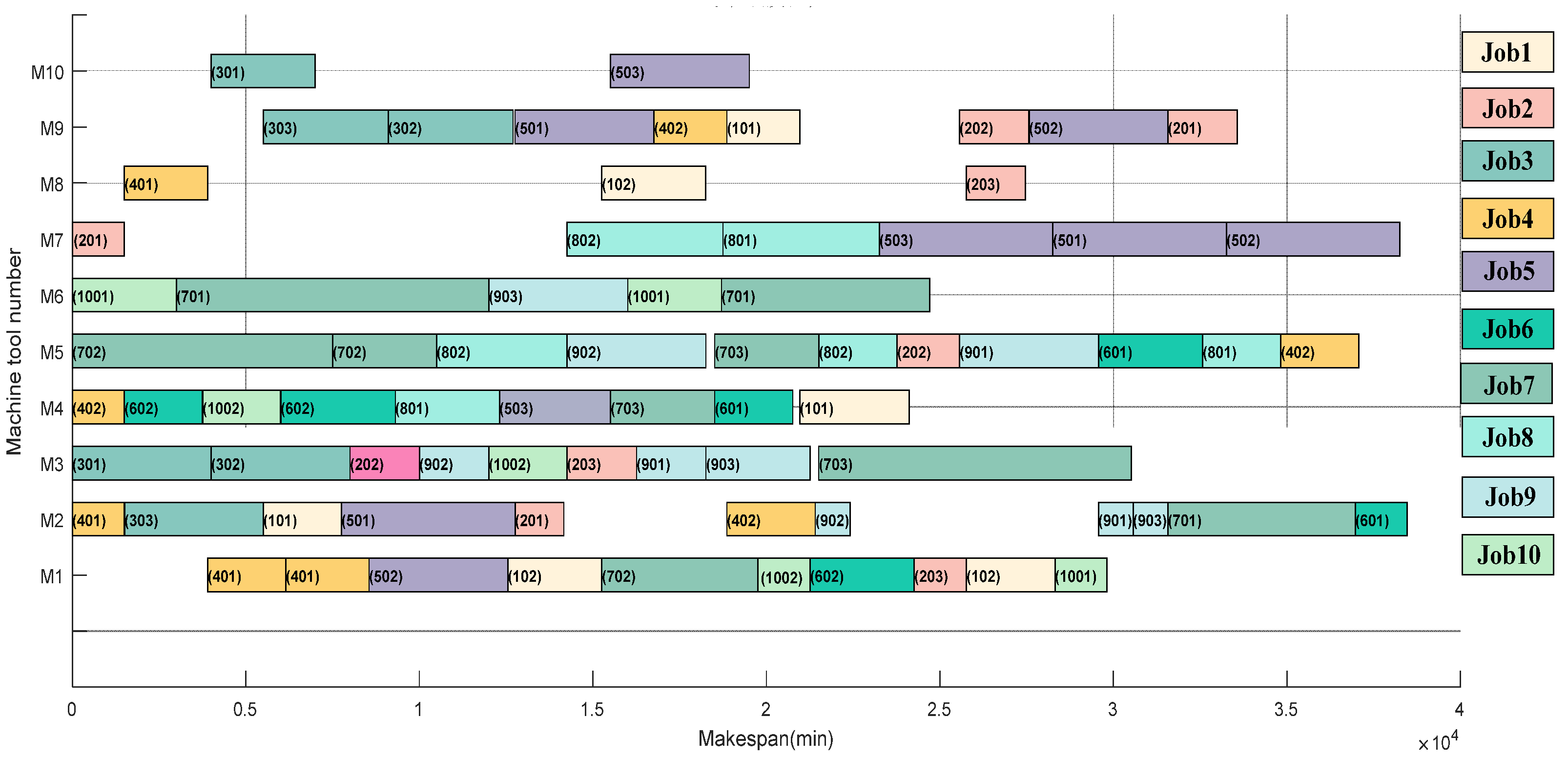
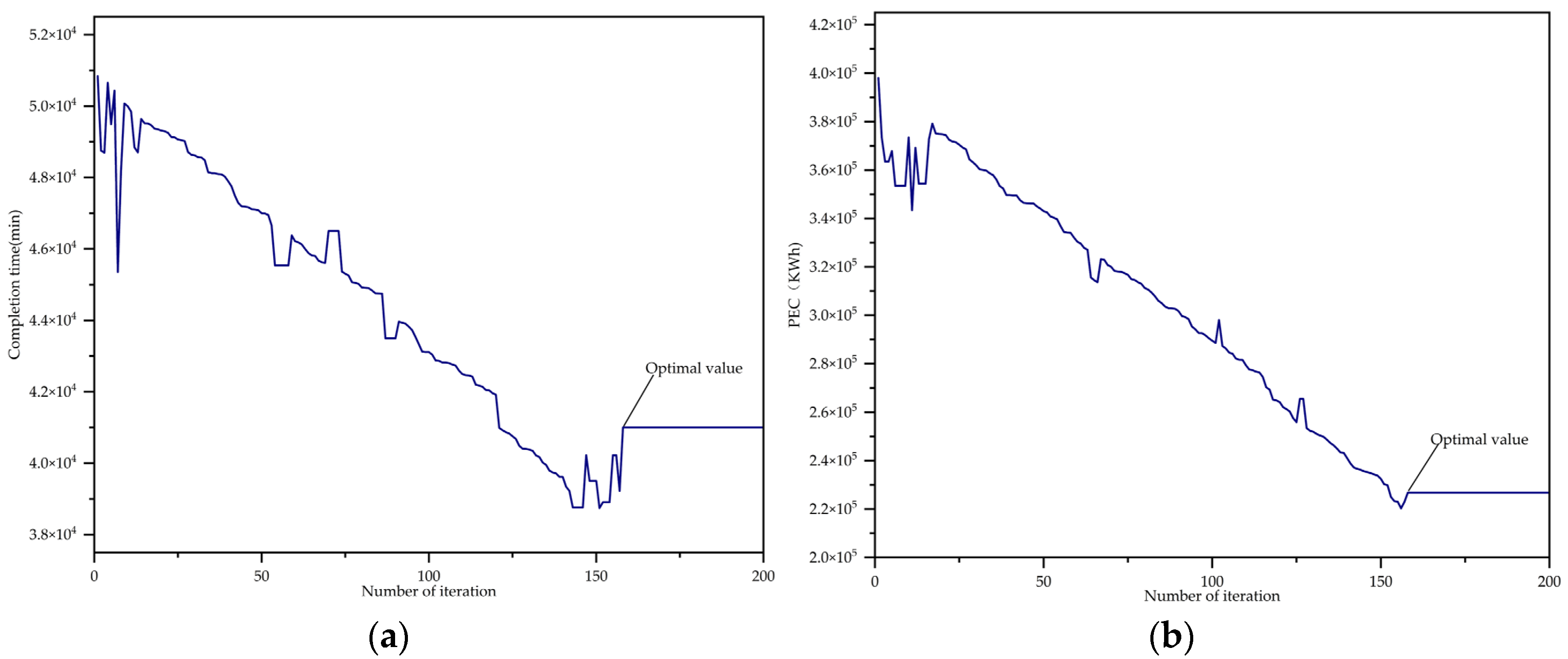
5.2. Result Analysis

In the experiment, taking into account the total energy consumption and completion time as the objective function and comprehensively considering all the energy consumption involved in the production process, the MOGWO algorithm was used to solve the problem. As shown in Figure 7, the values of the two optimization objectives stabilize at the 189th iteration. Figure 8a shows the population distribution results after 200 iterations. There are eight solutions set in Figure 8b. The point with lower energy consumption and early completion time than others was a selection in Figure 8b. The Gantt chart of this scheme is shown in Figure 9. As the total energy consumption optimization reduces the equipment conversion and waiting time, the completion time is 38,400.86 min, and the total energy consumption is 356,750 kWh.

Table 5. One sub-batch handling process for each kind of workpiece.

J01	Quantity	Operations	M	H	Start Time (min)	End Time (min)	Starting Location	Arrival Location
(J1) 101	150	O11	M2	H1	7756	7756.5	M2	M9
		O12	M9	H1	20,907.5	20,907.8	M9	M4
		O13	M4	H2	24,058	24,064.5	M4	P
(P1) 201	100	O21	M7	H2	2250	2250.5	M7	M2
		O22	M2	H2	14,861	14,861.5	M2	M9
		O23	M9	H3	33,914	33,920.5	M9	P
(P2) 301	200	O31	M3	H2	4004	4004.5	M3	M10
		O32	M10	H3	7007.5	7014	M10	P
(P3) 401	150	O41	M2	H2	1500	1500.5	M2	M8
		O42	M8	H2	3100.5	3101	M8	M1
		O43	M1	_	4601	4601	M1	M1
		O44	M1	H1	6201	6207.5	M1	P
(J2) 501	200	O51	M2	H3	12,759	12,759.5	M2	M9
		O52	M9	H3	16,759.5	16,759.7	M9	M7
		O53	M7	H2	33,118	33,124.5	M7	P
(J3) 601	150	O61	M4	H1	21,115	21,115.1	M4	M5
		O62	M5	H2	32,564	32,564.4	M5	M2
		O63	M2	H1	38,965	38,971.5	M2	P
(P4) 701	300	O71	M6	-	12,005	12,005	M6	M6
		O72	M6	H2	24,710	24,710.5	M6	M2
		O73	M2	H3	37,464	37,470.5	M2	P
(J4) 801	150	O81	M4	H1	11,751	11,751.3	M4	M7
		O82	M7	H1	23,224	23,224.2	M7	M5
		O83	M5	H2	34,817	34,823.5	M5	P
(J5) 901	200	O91	M3	H2	18,865	18,865.3	M3	M5
		O92	M5	H2	29,560	29,560.4	M5	M2
		O93	M2	H2	30,560.4	30,566.9	M2	P
(J6) 1001	150	O101	M6	-	3003	3003	M6	M6
		O102	M6	H2	18,708	18,708.5	M6	M1
		O103	M1	H2	29,572	29,579.5	M1	P

displays the handling process of the first sub-batch of each workpiece between the machines and the workshop, where J01 (J = 1, 2, 3, …,10) represents the first sub-batch of the Jth workpiece.

5.3. Comparison Analysis

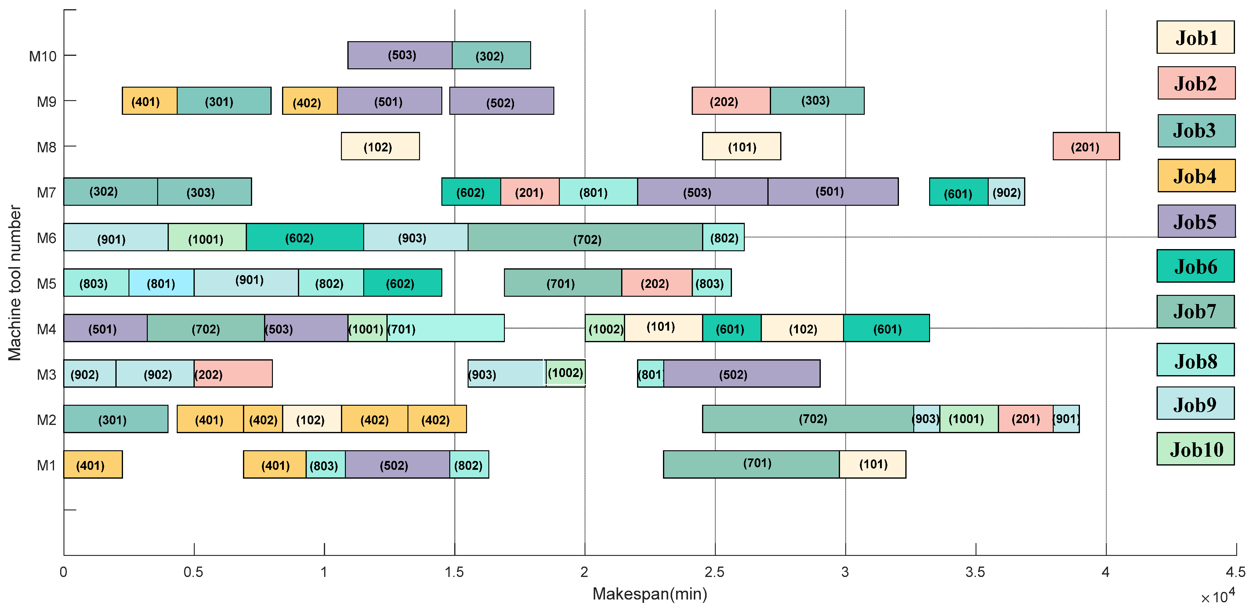
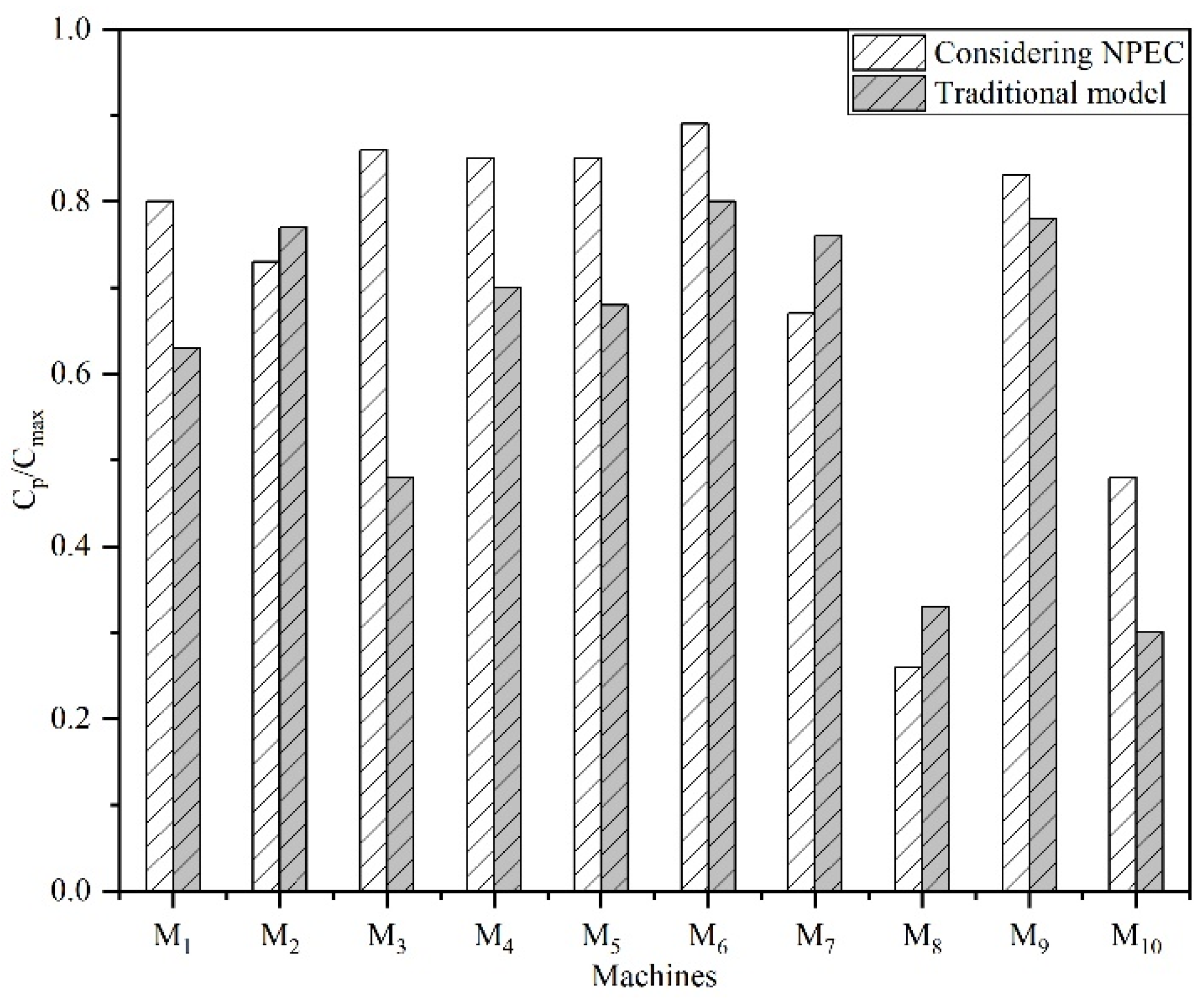
5.3.1. Comparison with the Traditional Model without Considering the NPEC

Different from the experiment above, only PEC is considered in the energy consumption model in this section. As shown in Figure 10, the values of the two optimization objectives stabilize at the 158th iteration. Figure 11a shows the population distribution results after 200 iterations. There are 10 solutions set in Figure 11b. The point with lower energy consumption and earlier completion time than others is selected in Figure 11b. The Gantt chart of this scheme is as shown in Figure 12, the total completion time is 40,900.43 min, and the PEC is 227,000 kWh.

Table 6. Comparison of energy consumption and time of two experiments. (unit: kWh).

	Optimize (PEC + NPEC)	Optimize PEC
Ep	2.33 $\times$ 105	2.27 $\times$ 105
Ew	4.75 $\times$ 104	5.33 $\times$ 104
Es	550	588
Ed	1.57 $\times$ 104	2.02 $\times$ 104
C	38,400.86	40,900.43

displays the energy consumption values and completion times for the two optimization schemes. As could be seen from the table, owing to the reduced standby and conversion time, the total completion time is better than that of the comparative experiment; in terms of energy consumption, the PEC values of the two schemes are very close; the slight difference in processing times may be owing to the different preparation times required on different equipment. The optimization of the handling equipment is not considered in the comparative experiment. The handling energy consumption in the comparative experiment is estimated through the historical handling time, and the energy consumption in our experiment is optimized. As could be seen in Table 6, the optimization of the handling energy consumption can significantly reduce the NPEC, thereby reducing the total energy consumption. Compared to the comparative experiment, the standby energy consumption and handling energy consumption are reduced by 9.95% and 22.28%, respectively. The utilization rates of each machine in the two experiments are shown in Figure 13. It can be seen from the figure that the machine utilization is mostly higher than that in the comparative experiment.

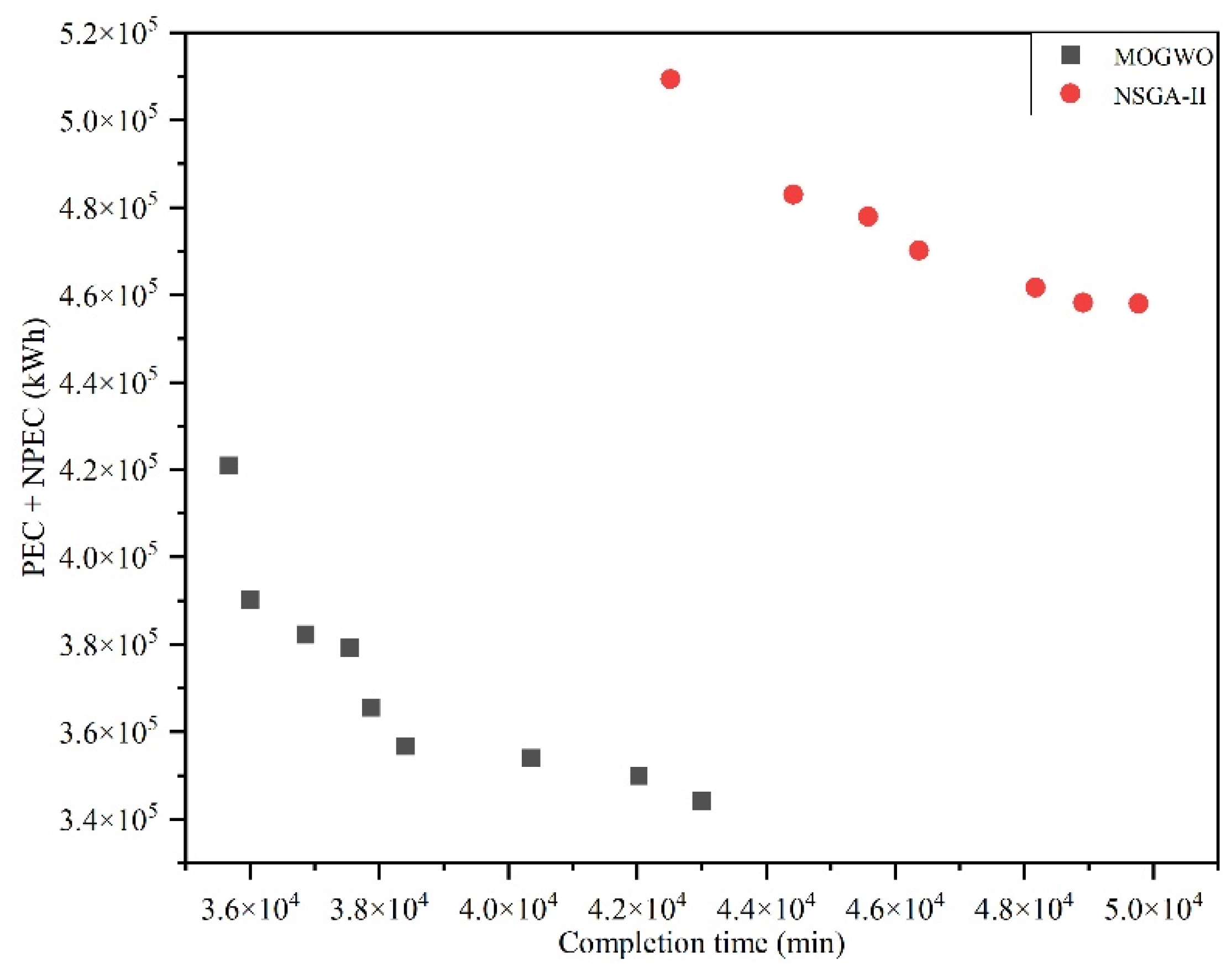
5.3.2. Algorithm Comparison with the NSGA-II

In this section, the most popular multi-objective heuristic algorithm NSGA-II [39] was selected in the experiment for comparative analysis. NSGA-II is an improvement of the NSGA algorithm. It is one of the most outstanding evolutionary multi-objective optimization algorithms so far. The parameters of the algorithm are set as follows: the population size is 100, the maximum number of iterations is set to G = 200, crossover probability Pc = 0.9, and the mutation probability Pm = 0.2. The parameters of MOGWO are set in Section 5.1. They use the same initialization strategy and encoding scheme.

Comparing the performance of multi-objective optimization algorithms is more based on the following criteria: (a) the degree of similarity between the solution set obtained by the operation result and the real Pareto solution set, that is, convergence; (b) the uniformity of the solution set on the Pareto frontier, namely diversity; (c) comprehensively measuring convergence and diversity. According to references [40,41], the following two indicators are used for algorithm performance evaluation: Δ metric and inverted generational distance. The real Pareto frontier of the research in this paper is the set of non-dominated solutions in the final solution set. However, the real Pareto frontier is not known. The final solution set is obtained by the calculation example through multiple independent operations of the algorithm. The specific introduction and calculation formula of these two indicators are given below.

Δ metric: Describe the uniformity of the Pareto front obtained by the algorithm. The calculation method is as follows. The smaller ∆, the more even the solution is, and the better the performance of the algorithm. When ∆ is equal to 0, it indicates that the solution obtained by the algorithm is uniformly distributed in the solution set space, generally only appearing under ideal circumstances.

$$\Delta =\frac{d_f+d_t+{\displaystyle \sum }_{i=1}^{n-1}|d_i-\overline{d}|}{d_f+d_t+(n-1)\overline{d}}$$

(27)

Here, d_f and d_t are the distances between the boundary point of the Pareto frontier obtained by the algorithm and the actual Pareto frontier boundary point of the problem to be solved; n represents the number of solutions in the Pareto frontier obtained by the algorithm operation, and d_i represents the value obtained by the algorithm operation. $\overline{d}$ represents the average value of all d_t.

Inverted generational distance: A variant of iterative distance not only reflects the convergence of the algorithm but also shows a diversity index, which is a comprehensive evaluation index. The formula of IGD is as follows:

$$\mathit{IGD}(S, P*)=\frac{{{\displaystyle \sum }}_{x\in P^{*}}\mathit{dist}(x,S)}{\left|P^{*}\right|}$$

(28)

Among them, dist(x, S) represents the individual x$\in$P* to the nearest Euclidean distance on S, and |P*| is the cardinality of the set P*. The smaller the value of IGD, the more it can approach the entire PF. In addition, when IGD(S, P*) = 0, it means S is a subset of P*.

In this paper, two intelligent optimization algorithms are selected for comparison. The results are shown

Table 7. Comparison of two algorithms.

Evaluation Index	MOGWO			NSGA-II
	Min	Agv	Sd	Min	Agv	Sd
Spread	0.343	0.553	0.107	0.522	0.677	0.115
Inverted generational distance	0.074	0.089	0.021	0.090	0.125	0.029

. The table counts the minimum, average, and standard deviation of the indicators.

From Table 7, we can draw the following two points:

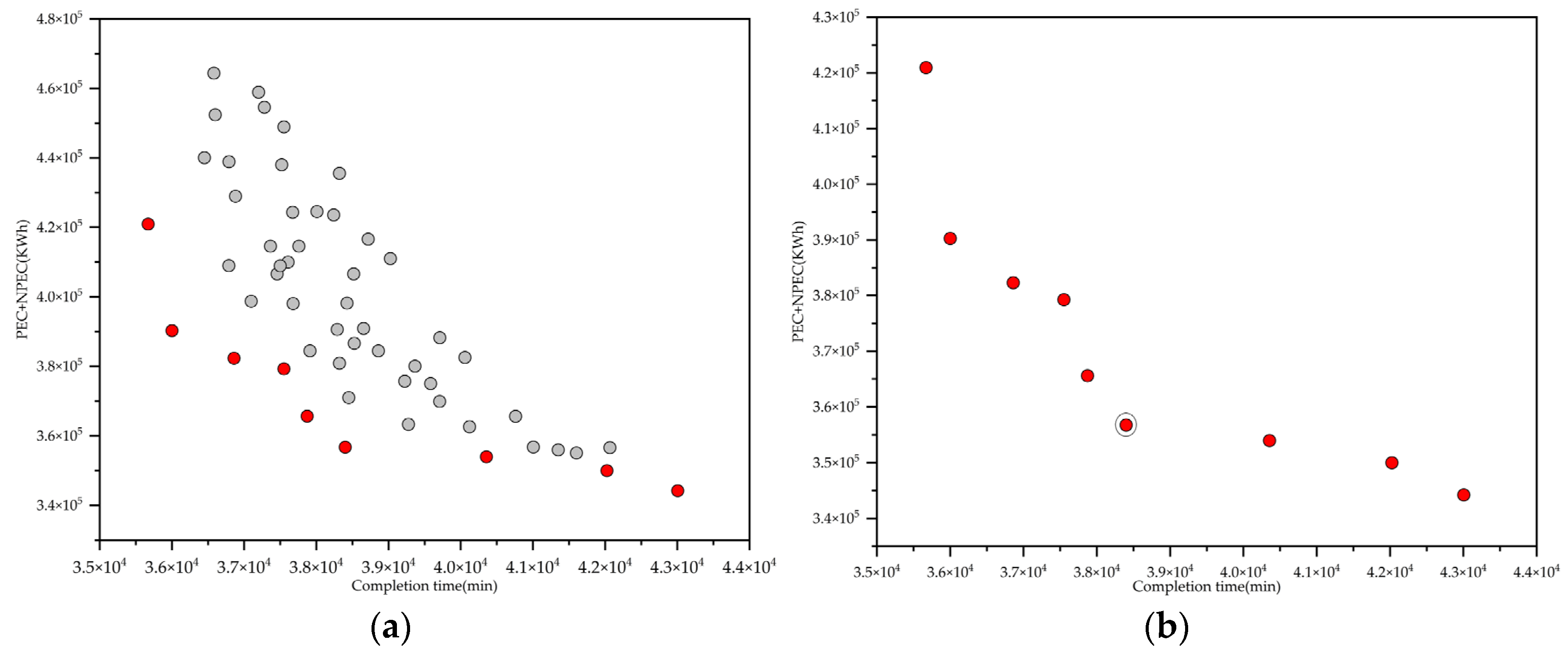
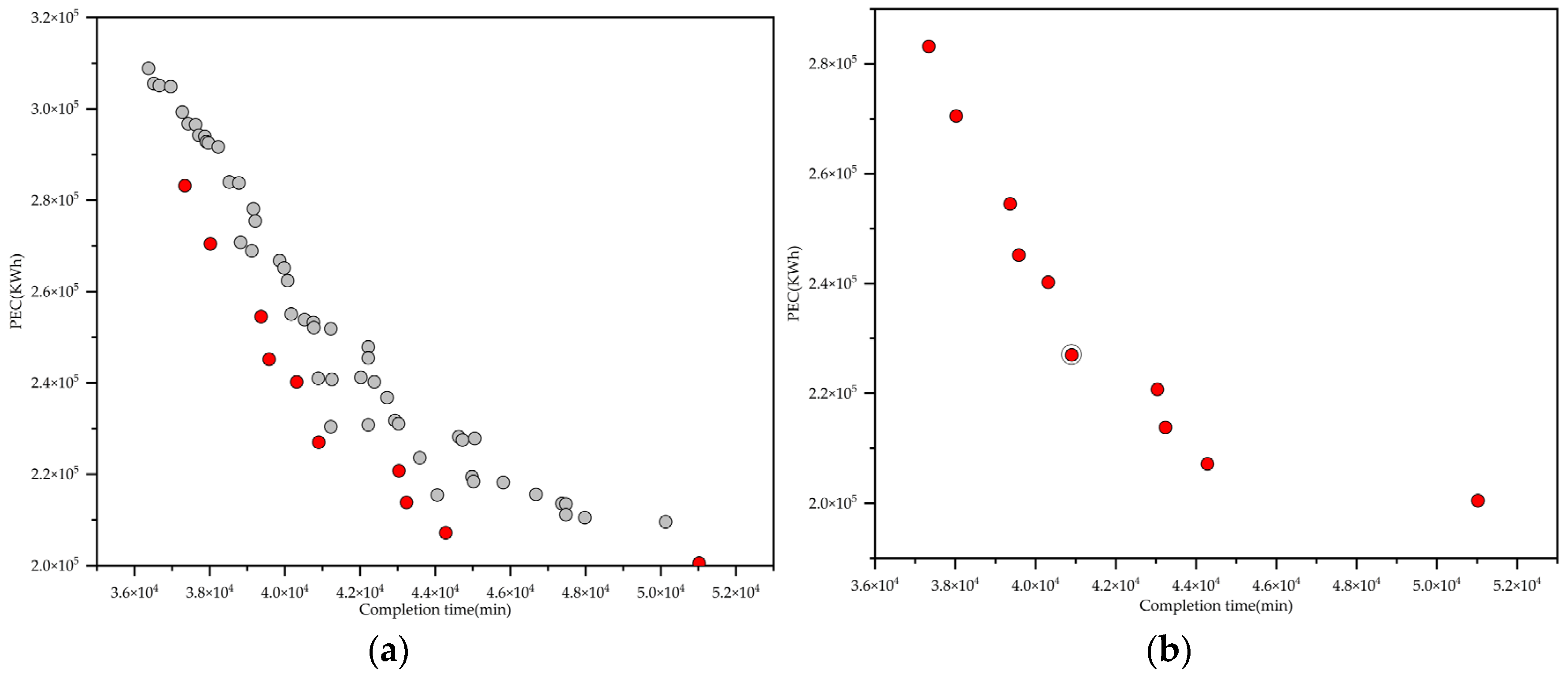
• According to the spread value (∆) in the table, MOGWO is better than the NSGA-II algorithm, and the MOGWO algorithm is more evenly distributed than the solution set obtained by NSGA-II. It is due to the neighborhood search mechanism of the MOGWO, which can increase the probability of obtaining the optimal solution, thereby improving the uniformity of the solution set distribution, and the algorithm has better optimization capabilities.
• According to the inverted generational distance value in the table, the solution obtained by MOGWO has better convergence and distribution than the NSGA-II algorithm. This is because of the unique hierarchical system of the MOGWO algorithm, which can be selected from different dominance levels. The optimal solution to improve the convergence and distribution of the algorithm was chosen.

The Pareto frontiers obtained by the two algorithms are shown in Figure 14. Observation shows that the solution obtained by using the MOGWO algorithm is numerically smaller than the other solution set, that is, it can dominate the solutions obtained by NSGA-II. Additionally, MOGWO proves to be effective in reducing the total energy consumption of scheduling plans. Therefore, the selected algorithm has the best solution effect.

5.4. Sensitivity Analysis

Sensitivity analysis was used to compare the influence of energy consumption of different auxiliary production operations in this section. If the objective function value and fitness value of different optimization operations change greatly, the sensitivity coefficient and the corresponding auxiliary production operation will be large and sensitive.

Sensitivity analysis is the importance of factor variables of the model to the value of the optimization objective function. The calculation is shown in Equation (29), as follows.

$$S_{\mathit{fA}}=\frac{\Delta f /f}{\Delta A / A}$$

(29)

Here, S_fA represents the sensitivity of target function value f to parameter A, and ΔA/A means the rate of change of a parameter; Δf/f represents the change rate of the target function value caused by the change of factor variable ΔA. The sensitivity of total energy consumption to E_W, E_s, and E_d will be analyzed in our experiment. In this analysis, ΔA/A represents the rate of change relative to historical observations when different auxiliary operation optimizations are considered. The change rate of total energy consumption due to different auxiliary operations of optimization is expressed by Δf/f.

Table 8. Sensitivity coefficients under different optimization combinations.

Schemes	MOGWO			ΔA/A	Δf/f	SfA
	Ew	Es	Ed
A	5.33 × 104	588	2.02 × 104	-	-	-
A1	4.63 × 104	-	-	13.13%	2.32%	0.18
A2	-	523	-	11.05%	0.22%	0.02
A3	-	-	1.49 × 104	26.24%	1.76%	0.07

shows the sensitivity coefficients under different optimization schemes; the larger the sensitivity coefficient, the higher the sensitivity of the target to the variation of parameters.

Table 8 compares the changes in total energy consumption when considering different combinations of auxiliary optimization operations. Among them, A represents the scheduling scheme without considering auxiliary operation optimization, where E_w, E_s, and E_d are historical forecast values. The standby time, conversion operation, and handling operation are considered separately, and the scheme is expressed by A₁, A₂, and A₃, respectively. Data indicate the three sensitivity coefficients are all positive and the target function value has a certain sensitivity to parameter changes, proving that the optimization model proposed in our research can obtain satisfactory results in reducing energy consumption, but there have been slightly different changes in the target function to the parameter between three schemes. From Table 8, energy consumption is significantly reduced by optimizing standby time, and the target quantity changes significantly to E_w; second is handling energy consumption optimization, followed by conversion energy consumption. In this research, due to the large standby time and handling times, the energy consumption optimization effect is relatively significant, especially in the case of large total energy consumption. Through the sensitivity analysis of the above optimization scheme, it is reasonable and effective to comprehensively consider the NPEC in the optimization model.

6. Conclusions and Future Works

This study researched energy consumption optimization in the production process of a machining workshop, starting from the assembly relationship between the parts/components of the multi-level product structure. By analyzing the existing energy consumption research, we conducted a systematic study on the NPEC of the workshop. The research was mainly conducted from the following two aspects.

• The production of a multi-level product structure is combined with energy consumption optimization. The start processing times of different levels of workpieces are set, and the characteristics of the PEC and NPEC in the production system are considered. With the goal of minimum completion time and energy consumption, equipment standby, workpiece conversion, and handling constraints are established, and the MOGWO is adopted to solve the problem.
• The total energy consumption optimization results are compared with those of an optimization plan considering only the PEC. The results show that after considering the NPEC optimization as proposed here, the standby energy consumption and handling energy consumption are reduced by 9.95% and 22.28%, respectively. This provides a feasible research direction for the study of energy-saving scheduling in workshops.

Production scheduling considering energy-saving measures is of great significance for the realization of energy savings and emissions reduction. This study has a set of limitations: for example, we suppose the same power during the standby time and there is no interruption in the processing that limit the versatility of our method. For future works, other possibilities, such as equipment failures and emergency order insertions, will be further integrated into the optimization model.

References

1. Pinedo, M.L. Scheduling: Theory, Algorithms, and Systems; Springer: New York, NY, USA, 2016. [Google Scholar]
2. Shi, F.; Zhao, S.K.; Meng, Y. Hybrid algorithm based on improved extended shifting bottleneck procedure and GA for assembly job shop scheduling problem. Int. J. Prod. Res. 2019, 1, 89–100. [Google Scholar] [CrossRef]
3. Pereira, M.T.; Santoro, M.C. An integrative heuristic method for detailed operations scheduling in assembly job shop systems. Int. J. Prod. Res. 2011, 49, 6089–6105. [Google Scholar] [CrossRef]
4. Kumar, M.L.; Kaur, J.; Singh, J. Dynamic and static energy efficient scheduling of task graphs on multiprocessors: A Heuristic. IEEE Access 2020, 8, 176351–176362. [Google Scholar] [CrossRef]
5. Jiang, Z.P.; Gao, D.; Lu, Y.; Kong, L.H.; Shang, Z.D. Electrical energy consumption of CNC machine tools based on empirical modeling. Int. J. Adv. Manuf. Technol. 2019, 100, 2255–2267. [Google Scholar] [CrossRef]
6. Li, K.Q. Energy and time constrained scheduling for optimized quality of service. Sust. Comput. 2019, 22, 134–138. [Google Scholar] [CrossRef]
7. Dahmus, J.B.; Gutowski, T.G. An environmental analysis of machining. In Proceedings of the ASME 2004 International Mechanical Engineering Congress and Exposition, Manufacturing Engineering and Materials Handling Engineering, Anaheim, CA, USA, 13–19 November 2004; pp. 643–652. [Google Scholar]
8. Xie, J.; Cai, W.; Du, Y.B.; Tang, Y.; Tuo, J.B. Modelling approach for energy efficiency of machining system based on torque model and angular velocity. J. Clean. Prod. 2021, 293, 126249. [Google Scholar] [CrossRef]
9. Jia, S.; Yuan, Q.; Lv, J.; Liu, Y.; Ren, D.; Zhang, Z. Therblig-embedded value stream mapping method for lean energy machining. Energy 2017, 138, 1081–1098. [Google Scholar] [CrossRef] [Green Version]
10. Mirjalili, S.; Mirjalili, S.M.; Lewis, A. Grey wolf optimizer. Adv. Eng. Softw. 2014, 69, 46–61. [Google Scholar] [CrossRef] [Green Version]
11. Saxena, A.; Soni, B.P.; Kumar, R.; Gupta, V. Intelligent grey wolf optimizer development and application for strategic bidding in uniform price spot energy market. Appl. Soft Comput. 2018, 69, 1–13. [Google Scholar] [CrossRef]
12. Miao, D.; Chen, W.; Zhao, W.; Demsas, T. Parameter estimation of PEM fuel cells employing the hybrid grey wolf optimization method. Energy 2020, 193, 571–582. [Google Scholar] [CrossRef]
13. Sattar, M.K.; Ahmad, A.; Fayyaz, S.; Ul Haq, S.S.; Saddique, M.S. Ramp rate handling strategies in Dynamic Economic Load Dispatch (DELD) problem using Grey Wolf Optimizer (GWO). J. Chin. Inst. Eng. 2019, 43, 200–213. [Google Scholar] [CrossRef]
14. Zhou, J.G.; Huo, X.J.; Xu, X.L.; Li, Y.S. Forecasting the carbon price using extreme-point symmetric mode decomposition and extreme learning machine optimized by the Grey Wolf Optimizer Algorithm. Energies 2019, 12, 950. [Google Scholar] [CrossRef] [Green Version]
15. Gokuldhev, M.; Singaravel, G.; Mohan, N.R. Ram. Multi-Objective local pollination-based Gray Wolf Optimizer for task scheduling heterogeneous cloud environment. J. Circuits Syst. Comput. 2020, 29, 2050100. [Google Scholar] [CrossRef]
16. Lu, C.; Gao, L.; Li, X.; Xiao, S. A hybrid multi-objective grey wolf optimizer for dynamic scheduling in a real-world welding industry. Eng. Appl. Artif. Intell. 2017, 57, 61–79. [Google Scholar] [CrossRef]
17. Qin, H.B.; Fan, P.F.; Tang, H.T.; Huang, P.; Fang, B.; Pan, S.F. An effective hybrid discrete grey wolf optimizer for the casting production scheduling problem with multi-objective and multi-constraint. Comput. Ind. Eng. 2019, 128, 458–476. [Google Scholar] [CrossRef]
18. Luo, S.; Zhang, L.X.; Fan, Y.S. Energy-efficient scheduling for multi-objective flexible job shops with variable processing speeds by grey wolf optimization. J. Clean Prod. 2019, 234, 1365–1384. [Google Scholar] [CrossRef]
19. Paul, M.; Ramanan, T.R.; Sridharan, R. Simulation modelling and analysis of dispatching rules in an assembly job shop production system with machine breakdowns. Int. J. Adv. Manuf. Technol. 2018, 3, 234–251. [Google Scholar] [CrossRef]
20. Hongbum, N.; Jinwoo, P. Multi-level job scheduling in a flexible job shop environment. Int. J. Prod. Res. 2014, 52, 3877–3887. [Google Scholar]
21. Li, Y.J.; Liu, J.J.; Chen, Q.X.; Mao, N. Lot splitting and scheduling algorithm of multi-level assembly job shops. Compu. Integr. Manuf. Syst. (accepted).
22. Lu, H.; He, L.; Huang, G.Q.; Wang, K. Development and comparison of multiple genetic algorithms and heuristics for assembly production planning. IMA J. Manag. Math. 2014, 27, 181–200. [Google Scholar] [CrossRef]
23. Wan, F.; Liu, J.H.; Ning, R.X.; Zhuang, C.B. Visual production scheduling technology for the complex product assembly process. Compu. Inte. Manuf. Syst. 2013, 19, 755–765. [Google Scholar]
24. Suharyanti, Y.; Ariyono, V. The effect of product structure complexity and process complexity on optimum lot size in multilevel product scheduling. In Proceedings of the Asia Pacific Industrial Engineering and Management Systems (APIEMS) Conference, Melaka, Malaysia, 7–10 December 2010. [Google Scholar]
25. Che, A.; Wu, X.Q.; Peng, J.; Yan, P.Y. Energy-efficient bi-objective single-machine scheduling with power-down mechanism. Comput. Oper. Res. 2017, 85, 172–183. [Google Scholar] [CrossRef]
26. Twomey, J.; Yildirim, M.B.; Whitman, L.; Liao, H.; Ahmad, J. Energy Profiles of Manufacturing Equipment for Reducing ConSumption in a Production Setting; Working Paper; Wichita State University: Wichita, KS, USA, 2008. [Google Scholar]
27. Wang, X.L.; Luo, W.; Zhang, H.; Dan, B.B.; Feng, L. Energy consumption model and its simulation for manufacturing and remanufacturing systems. Int. J. Adv. Manuf. Technol. 2016, 87, 1557–1569. [Google Scholar] [CrossRef]
28. Luan, X.N.; Zhang, S.; Chen, J.; Li, G. Energy modelling and energy saving strategy analysis of a machine tool during non-cutting status. Int. J. Prod. Res. 2019, 57, 4451–4467. [Google Scholar] [CrossRef]
29. Liu, Y.; Dong, H.B.; Niels, L.; Sanja, P.; Nabil, G. An investigation into minimising total energy consumption and total weighted tardiness in job shops. J. Clean. Prod. 2014, 65, 87–96. [Google Scholar] [CrossRef]
30. Peng, C.; Peng, T.; Zhang, Y.; Tang, R.; Hu, L. Minimising non-processing energy consumption and tardiness fines in a mixed-flow shop. Energies 2018, 11, 3382. [Google Scholar] [CrossRef] [Green Version]
31. Wu, X.L.; Cui, Q. Multi-objective flexible flow shop scheduling problem with renewable energy. Compu. Inte. Manuf. Syst. 2018, 24, 144–159. [Google Scholar] [CrossRef]
32. Gilles, M.; Mehmet, B.Y.; Twomey, J. Operational methods for minimization of energy consumption of manufacturing equipment. Int. J. Prod. Res. 2007, 45, 4247–4271. [Google Scholar]
33. Wang, H.; Jiang, Z.G.; Wang, Y.; Zhang, H.; Wang, Y.H. A two-stage optimization method for energy-saving flexible job-shop scheduling based on energy dynamic characterization. J. Clean. Prod. 2018, 188, 575–588. [Google Scholar] [CrossRef]
34. Zhang, Q.; Manier, H.; Manier, M.A. A genetic algorithm with tabu search procedure for flexible job shop scheduling with transportation constraints and bounded processing times. Comput. Oper. Res. 2012, 39, 1713–1723. [Google Scholar] [CrossRef]
35. Zhao, N.; Li, K.D.; Tian, Q.; Du, Y.H. Fast optimization approach of flexible job shop scheduling with transport time consideration. Compu. Inte. Manuf. Syst. 2015, 21, 724–732. [Google Scholar]
36. Rahman, H.F.; Nielsen, I. Scheduling automated transport vehicles for material distribution systems. Appl. Soft. Comput. 2019, 82, 105552. [Google Scholar] [CrossRef]
37. Benton, W.C.; Srivastava, R. Product structure complexity and inventory storage capacity on the performance of a multi-level manufacturing system. Int. J. Prod. Res. 1993, 31, 2531–2545. [Google Scholar] [CrossRef]
38. Mirjalili, S.; Saremi, S.; Mirjalili, S.M.; Coelho, L.S. Multi-objective grey wolf optimizer: A novel algorithm for multi-criterion optimization. Expert Syst. Appl. 2016, 47, 106–119. [Google Scholar] [CrossRef]
39. Deb, K.; Pratap, A.; Agarwal, S.; Meyarivan, T. A fast and elitist multi-objective genetic algorithm: NSGA-II. IEEE Trans. Evol. Comput. 2002, 6, 182–197. [Google Scholar] [CrossRef] [Green Version]
40. Zhao, M.; Song, X.Y.; Chang, C.G. Improved artificial bee colony algorithm and its application on optimization of emergency scheduling. Appl. Res. Comput. 2016, 33, 3596–3601. [Google Scholar]
41. Bosman, P.; Thierens, D. The balance between proximity and diversity in multi-objective evolutionary algorithms. IEEE Trans. Evol. Comput. 2003, 7, 174–188. [Google Scholar] [CrossRef] [Green Version]
Figure 1. Three types of product structure.
Energies 14 06079 g001
Figure 2. Gantt chart of m and the distribution of corresponding power.
Energies 14 06079 g002
Figure 3. Multi-objective gray wolf algorithm flow chart.
Energies 14 06079 g003
Figure 4. Chromosome coding, for example.
Energies 14 06079 g004
Figure 5. Gantt chart of first sub-batch.
Energies 14 06079 g005
Figure 6. Product structure tree of tall.
Energies 14 06079 g006
Figure 7. Convergence process of two objectives: (a) convergence process of C objective; (b) convergence process of E objective.
Energies 14 06079 g007
Figure 8. Results obtained considering PEC+NPEC: (a) final population distribution; (b) Pareto frontier distribution.
Energies 14 06079 g008
Figure 9. Gantt chart of the optimized schedule scheme.
Energies 14 06079 g009
Figure 10. Convergence process of two objectives: (a) convergence process of C objective; (b) convergence process of PEC objective.
Energies 14 06079 g010
Figure 11. Results obtained in comparison experiment: (a) final population distribution; (b) Pareto frontier distribution.
Energies 14 06079 g011
Figure 12. Gantt chart of the optimized scheme from the traditional model.
Energies 14 06079 g012
Figure 13. Comparison in Cp/C for machines.
Energies 14 06079 g013
Figure 14. Comparison of two algorithms.
Energies 14 06079 g014