An Energy Management System for the Control of Battery Storage in a Grid-Connected Microgrid Using Mixed Integer Linear Programming

Abstract

This paper proposes an energy management system (EMS) for battery storage systems in grid-connected microgrids. The battery charging/discharging power is determined such that the overall energy consumption cost is minimized, considering the variation in grid tariff, renewable power generation and load demand. The system is modeled as an economic load dispatch optimization problem over a 24 h horizon and solved using mixed integer linear programming (MILP). This formulation, therefore, requires knowledge of the expected renewable energy power production and load demand over the next 24 h. To achieve this, a long short-term memory (LSTM) network is proposed. The receding horizon (RH) strategy is suggested to reduce the impact of prediction error and enable real-time implementation of the EMS that benefits from using actual generation and demand data on the day. At each hour, the LSTM predicts generation and load data for the next 24 h, the dispatch problem is then solved and the battery charging or discharging command for only the first hour is applied in real-time. Real data are then used to update the LSTM input, and the process is repeated. Simulation results show that the proposed real-time strategy outperforms the offline optimization strategy, reducing the operating cost by 3.3%.

1. Introduction

The development of microgrid (MG) technology has provided the opportunity and the infrastructure for improving the efficiency of energy consumption [1,2]. Microgrid systems are typically made up of load and distributed energy resources, such as photovoltaics (PV) systems, wind turbines, biogas power plants, fuel cells and energy storage systems (ESS) [3]. A microgrid can operate in a grid-connected or an islanded mode. The hybrid microgrid system, which comprises different distributed energy resources, has become promising as it provides an integral part of the development of smart grid systems [4,5]. However, there are still many challenges in implementing and operating the microgrid, one of which arises due to the intermittent nature of the renewable energy sources (RESs) because of the stochastic nature of the underlying metrological conditions [6]. A potential solution to this challenge is the integration of a fast-response energy storage system. Energy storage is an important component with great prospects in future power systems, as it plays an important role in alleviating the problem of sudden energy crisis and power shortage in remote areas [7]. Moreover, the introduction of the hybrid system enhances self-consumption and offers an opportunity to reduce energy costs. The EMS ensures the availability of energy resources during longer time intervals, ensuring that the load demand is met by the total power produced by the distributed energy resources [8].

Extensive research has been reported previously on the management of microgrids, much of which has focused on mathematical formulations and is usually tested under offline scenarios. However, due to the stochastic nature of the RESs, offline optimization may fail to achieve the optimal result as the uncertainties of the RESs are not considered in real-time. In [9], a linear mathematical model is suggested to balance the generation and load of a microgrid by minimizing the total operating cost of the system over 24 h. To demonstrate the performance of their approach, a tiered power management system composed of an advisory and a real-time layer was introduced. The advisory layer provided long-term directives to the real-time layer by solving the RH problem offline using the predicted PV and load data. However, this approach was not implemented in real-time using real data; instead, long-term directives from the advisory layer were passed to the real-time layer. In [10], the economic dispatch problem for total operation and cost minimization in a DC-MG has been formulated and solved with a heuristic method. However, this approach does not enhance the design of the EMS architecture so that it can be easily implemented on a physical system. An intelligent energy management system is defined in [11] as an architecture that sequentially connected functional modules such as power forecasting, energy storage management and an optimization module for a day-ahead optimal operation of the microgrid. However, this system may produce a bottleneck in the flow of data for real-time operations. These reported works do not deal with the uncertainty of the RESs generation nor the consumption in real-time. To overcome these challenges, an online strategy such as the one proposed in [12,13] can be implemented, where energy management systems are designed and implemented by considering the current status of the microgrid, but without consideration of future power generation or load demand. In [14], an optimal energy/power control method is presented for the operation of energy storage in grid-connected MGs considering forecast electricity usage and renewable energy generation. However, prediction errors due to long-term predictions were not considered. In [15], a rolling horizon-based energy management strategy is defined for a specific case study. The strategy consists of two stages: a deterministic management model is first formulated, followed by a rolling horizon control strategy. The actions on the microgrid devices respond to an optimization criterion related to the estimation of the future system behavior, which is continually predicted by updatable forecasts to reduce uncertainty in both production capacity and energy demand. However, the proposed optimization model did not consider the control of the ESS in real-time utilizing the predicted PV generation and load demand within the 24-hour time horizon. To address this issue, the current work pays attention to operating the EMS in real-time utilizing the LSTM network, because of its long-term memory for the prediction of variables in systems such as PV generation and load demand.

In this paper, the RH control strategy is utilized to perform the optimization every hour and the LSTM predicts the PV generation and load data for 24 h. The optimal dispatch problem is solved using the MILP algorithm and the dispatchable battery commands for the first hour are applied in real-time. The real data are then used to update the LSTM input and the process is repeated for future time windows. With this approach, the EMS can mitigate the undesirable challenges associated with the PV generation’s stochasticity and real-time power imbalances.

To evaluate the proposed approach, the daily operating cost is compared against a reference benchmark. The proposed hybrid MILP-LSTM optimization framework is executed in two different scenarios:

• Online Optimization—Execution every hour in real-time using a receding horizon of 24 h.
• Offline Optimization—Execution once a day using a single set of LSTM-predicted data.

Simulations have been carried out for different operating conditions covering 12 months.

The microgrid optimal performance is dependent on the ESS charging/discharge times based on the time of use (ToU) tariff of the grid. It is evaluated in terms of the daily operating cost of energy [9]. The optimal schedule of the grid-connected microgrid is performed through the optimization of the microgrid. The MILP optimization approach is chosen because it presents a flexible and robust method for solving complex problems by making fast energy management decisions via integer decision variables and identifying the best connection between the plants and utilities. It systematically finds the best trade-off in the operation of the microgrid to achieve maximum resource efficiency and minimum operating cost while respecting the system operational constraints [16]. We have utilized the LSTM-MILP-RH control strategy for the optimization of the grid-connected microgrid while introducing new constraints for controlling the ESS charge/discharge cycle, using the most up-to-date predictions and the latest information about the system, to adapt to new events and operating conditions. The LSTM-MILP-RH (online) approach was compared against the LSTM-MILP (offline) approach, demonstrating that the online optimization approach outperforms the offline approach, and the results are presented in Section 4.

Table 1. Table of comparison between proposed method and other methods available in the literature.

References	Contribution/Application	Method Used
[9]	Power management and operating cost minimization	MILP, Tiered Power Management System
[10]	Economic dispatch and cost minimization	MILP and Heuristic Method
[11]	Day-ahead optimal operation of microgrid	Mathematical Modeling
[13]	Real-time operation of microgrids	MILP
[14]	Optimal energy/power control	Mathematical Modeling
[15]	Deterministic management model with two-stage energy management model	Rolling horizon-based energy management strategy, MILP
This paper	Energy management, battery control (charge/discharge cycle) and operating cost minimization.	Offline and online optimization approach using MILP with receding horizon control (LSTM-MILP-RH approach)

compares the contribution of this paper in terms of other similar methodologies in the contemporary literature.

The rest of the paper is organized as follows: Section 2 presents the proposed optimal operation of the battery in a grid-tied microgrid, the MILP formulation and LSTM prediction theory. The RH control strategy implementation is explained in Section 3. In Section 4, the simulation results are presented, and the conclusion is drawn in Section 5.

2. Optimal Operation of Battery Using MILP

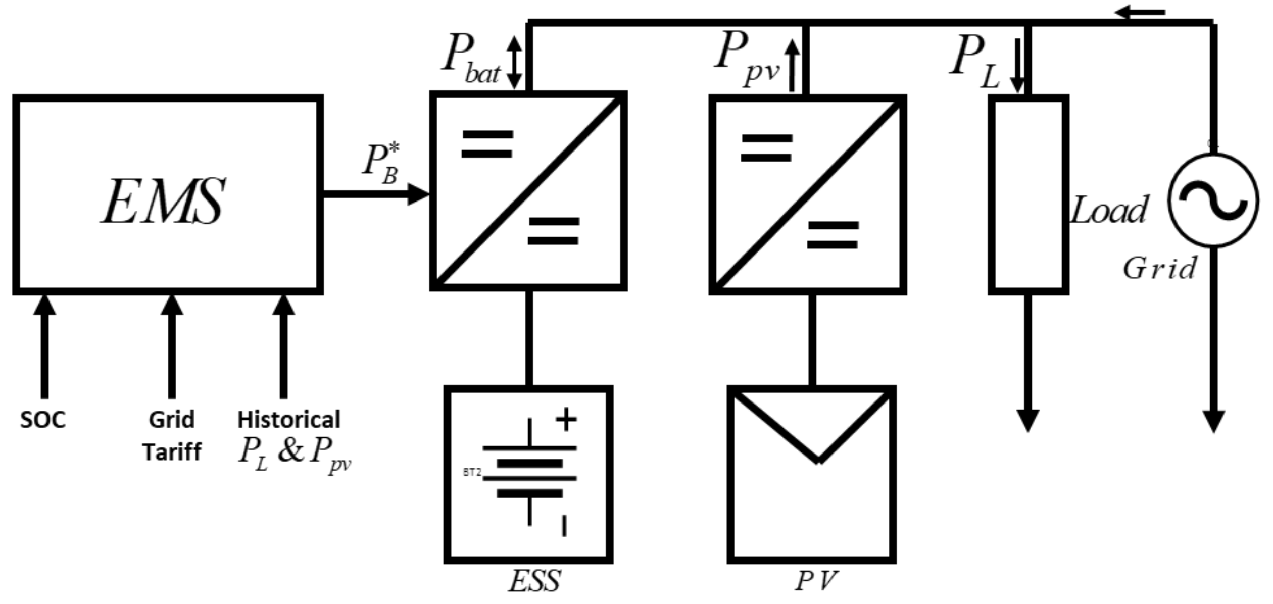
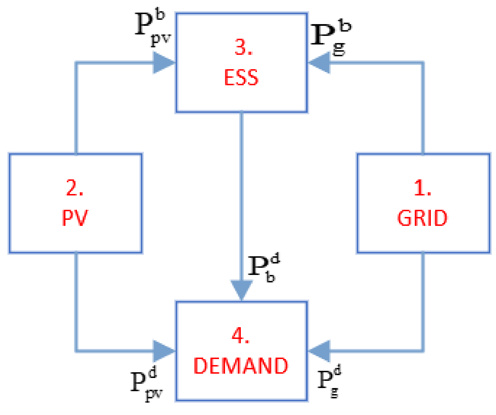
A schematic of the grid-tied microgrid under study is shown in Figure 1. The main components of the hybrid system are the PV, ESS and local load. The power flow within the microgrid is illustrated in Figure 2. The grid connection is represented in the first node and the imported power from the grid, ${\mathrm{P}}_{\mathrm{g}}\left(\mathrm{t}\right)$, at time $\mathrm{t}$ is used for the charging of the ESS in the third node and directly supplies the load demand in the fourth node. The second node is the PV supply source, which can also be used to charge the ESS and supply the load demand. The energy demand at all times is met by a combination of power from the PV, denoted as ${\mathrm{P}}_{\mathrm{p}\mathrm{v}}\left(\mathrm{t}\right)$ power from the ESS, ${\mathrm{P}}_{\mathrm{b}}$, and power from the grid, as described in (1):

$${\mathrm{P}}_{\mathrm{d}}\left(\mathrm{t}\right)={\mathrm{P}}_{\mathrm{p}\mathrm{v}}\left(\mathrm{t}\right)+{\mathrm{P}}_{\mathrm{g}}\left(\mathrm{t}\right)+{\mathrm{P}}_{\mathrm{b}}^{\mathrm{d}}\left(\mathrm{t}\right)-{\mathrm{P}}_{\mathrm{b}}^{\mathrm{c}\mathrm{h}}(\mathrm{t}),$$

(1)

The PV generation should supply the energy demand. When it is insufficient, additional power is imported from the ESS and/or the grid depending on the battery state of charge (SoC) and the grid tariff.

2.1. The MILP Formulation

The MILP is formulated to solve the economic dispatch problem to find the minimum operational cost while satisfying the load demand and respecting imposed constraints. The MILP economic dispatch problem solution results in the optimal power flow through each connection for each time step in the optimization horizon [17,18]. To formulate the microgrid scheduling problem, the cost function associated with the MILP and the constraints are defined in (2) as:

$$\begin{array}{l}\min \mathrm{Z}\hspace{0.33em}={\displaystyle \sum _{\mathrm{t}=0}^{\mathrm{T}}{\displaystyle \sum _{\mathrm{i}=1}^{\mathrm{N}}\mathrm{C}({\mathrm{P}}_{\mathrm{g}\mathrm{r}}(\mathrm{i},\mathrm{t})}}),\\ \mathrm{subjected} \mathrm{to}:\\ {\displaystyle \sum _{\mathrm{t}=0}^{\mathrm{N}}{\mathrm{P}}_{\mathrm{g}\mathrm{r}}(\mathrm{i},\mathrm{t})={\mathrm{P}}_{\mathrm{d}}\left(\mathrm{t}\right)} \in \mathsf{\vartheta }\left(\mathrm{i}\right),\end{array}$$

(2)

where $\mathrm{Z}$ is the objective function, $\mathit{N}$ is the number of generators in the power system, $\mathrm{C}({\mathrm{P}}_{\mathrm{g}\mathrm{r}}(\mathrm{i},\mathrm{t}))$ is the cost of the generated power by ${\mathrm{P}}_{\mathrm{g}\mathrm{r}}$ and $\mathsf{\vartheta }\left(\mathrm{i}\right)$ represents the set of constraints for ${\mathrm{P}}_{\mathrm{g}\mathrm{r}}$. The selected optimal solution is implemented on the system equations and the system response, such as the ESS state of charge, charge/discharge power is measured [9]. The decision variables for the economic dispatch problem are presented in

Table 2. Description of the decision variables and binary variables of the economic dispatch problem.

Decision Variable	Variable Type	Description
${\mathrm{P}}_{\mathrm{g}}^{\mathrm{d}}\left(\mathrm{t}\right)$	Continuous	Power from the Grid to the Load
${\mathrm{P}}_{\mathrm{g}}^{\mathrm{b}}\left(\mathrm{t}\right)$	Continuous	Power from the Grid to the ESS
${\mathrm{P}}_{\mathrm{p}\mathrm{v}}^{\mathrm{d}}\left(\mathrm{t}\right)$	Continuous	Power from PV to the Load
${\mathrm{P}}_{\mathrm{p}\mathrm{v}}^{\mathrm{b}}\left(\mathrm{t}\right)$	Continuous	Power from PV to ESS
${\mathrm{y}}_{\mathrm{b}}^{\mathrm{c}\mathrm{h}}\left(\mathrm{t}\right)$	Binary	On/off state of the ESS charge
${\mathrm{y}}_{\mathrm{b}}^{\mathrm{d}}\left(\mathrm{t}\right)$	Binary	On/off state of the ESS discharge
$\mathsf{\alpha }(\mathrm{t})$	Binary	Variable for the charging state of the ESS

.

The state of charge of the ESS and the charge/discharge powers from the ESS, ${\mathrm{P}}_{\mathrm{b}}^{\mathrm{d}}$, are calculated in terms of the decision variables and considered as the system state. For each time step, the total energy of the microgrid system is defined as ${\mathrm{P}}_{\mathrm{g}\mathrm{r}}\left(\mathrm{t}\right)\times \mathsf{\Delta }\mathrm{t}$. It is important that the optimization process does not schedule ESS charge and discharge simultaneously. Therefore, an inequality constraint is formulated as an integer in (3) as:

$${\mathrm{y}}_{\mathrm{b}}^{\mathrm{c}\mathrm{h}}\left(\mathrm{t}\right)+{\mathrm{y}}_{\mathrm{b}}^{\mathrm{d}}\left(\mathrm{t}\right)\le 1,$$

(3)

$$\left.\begin{array}{l}{\mathrm{P}}_{\mathrm{b}}^{\mathrm{d}}\left(\mathrm{t}\right)\le {\mathrm{P}}_{\mathrm{b}}^{\begin{array}{l}\mathrm{d}\\ \max \end{array}}\times {\mathrm{y}}_{\mathrm{b}}^{\mathrm{d}}(\mathrm{t})\\ {\mathrm{P}}_{\mathrm{b}}^{\mathrm{c}\mathrm{h}}\left(\mathrm{t}\right)\le {\mathrm{P}}_{\mathrm{b}}^{\begin{array}{l}\mathrm{c}\mathrm{h}\\ \max \end{array}}\times {\mathrm{y}}_{\mathrm{b}}^{\mathrm{c}\mathrm{h}}\left(\mathrm{t}\right)\end{array}\right\},$$

(4)

The power imported from the grid is formulated as:

$${\mathrm{P}}_{\mathrm{g}}\left(\mathrm{t}\right)\le {\mathrm{P}}_{\mathrm{g}}^{\max },$$

(5)

The grid and PV powers at any time $\mathrm{t}$ can be used to charge the ESS and feed the load. The flow in the network considers the storage capabilities of the ESS and the possible curtailment of the PV. This is represented by the node balance constraints given in (6)–(9) as:

$${\mathrm{P}}_{\mathrm{g}}(\mathrm{t})={\mathrm{P}}_{\mathrm{g}}^{\mathrm{d}}\left(\mathrm{t}\right)+{\mathrm{P}}_{\mathrm{g}}^{\mathrm{b}}\left(\mathrm{t}\right)$$

(6)

$${\mathrm{P}}_{\mathrm{p}\mathrm{v}}\left(\mathrm{t}\right)\ge {\mathrm{P}}_{\mathrm{p}\mathrm{v}}^{\mathrm{d}}\left(\mathrm{t}\right)+{\mathrm{P}}_{\mathrm{p}\mathrm{v}}^{\mathrm{b}}\left(\mathrm{t}\right),$$

(7)

$${\mathrm{P}}_{\mathrm{b}}^{\mathrm{c}\mathrm{h}}\left(\mathrm{t}\right)={\mathrm{P}}_{\mathrm{g}}^{\mathrm{b}}\left(\mathrm{t}\right)+{\mathrm{P}}_{\mathrm{p}\mathrm{v}}^{\mathrm{b}}\left(\mathrm{t}\right),$$

(8)

$${\mathrm{P}}_{\mathrm{b}}^{\mathrm{d}}\left(\mathrm{t}\right)={\mathrm{P}}_{\mathrm{d}}\left(\mathrm{t}\right)-{\mathrm{P}}_{\mathrm{p}\mathrm{v}}^{\mathrm{d}}\left(\mathrm{t}\right)-{\mathrm{P}}_{\mathrm{g}}^{\mathrm{d}}\left(\mathrm{t}\right),$$

(9)

Whenever the PV system produces power greater than the load demand, the excess power is utilized in charging the ESS depending on the SoC. The inequalities in (10) show that the power from the grid and the PV can only be positive parameters, represented as:

$$\left.\begin{array}{l}{\mathrm{P}}_{\mathrm{g}}\left(\mathrm{t}\right)\ge 0, {\mathrm{P}}_{\mathrm{p}\mathrm{v}}\left(\mathrm{t}\right)\ge 0\\ {\mathrm{P}}_{\mathrm{p}\mathrm{v}}^{\mathrm{b}}\left(\mathrm{t}\right)\ge 0, {\mathrm{P}}_{\mathrm{g}}^{\mathrm{b}}\left(\mathrm{t}\right)\ge 0\end{array}\right\},$$

(10)

The SoC of the ESS must be kept within a safety limit that is defined based on the minimum and maximum SoC of the battery, given in (11) as:

$${\mathsf{\beta }}_{\mathrm{soc}}^{\min }\le {\mathsf{\beta }}_{\mathrm{s}\mathrm{o}\mathrm{c}}\left(\mathrm{t}\right)\le {\mathsf{\beta }}_{\mathrm{soc}}^{\max },$$

(11)

To enforce (11), further constraints are developed in (12) and (13) relating the SoC to the capacity of the ESS and the power flows to and from the battery as:

$${\mathsf{\delta }}_{\mathrm{c}}{\mathsf{\beta }}_{\mathrm{soc}}(\mathrm{t})+{\mathrm{P}}_{\mathrm{b}}^{\mathrm{c}\mathrm{h}}(\mathrm{t}){\mathsf{\eta }}_{\mathrm{c}}\mathsf{\Delta }\mathrm{t}-{\mathrm{P}}_{\mathrm{b}}^{\mathrm{d}}(\mathrm{t}){\mathsf{\eta }}_{\mathrm{d}}\mathsf{\Delta }\mathrm{t}\le {\mathsf{\delta }}_{\mathrm{c}}$$

(12)

$${\mathsf{\delta }}_{\mathrm{C}}{\mathsf{\beta }}_{\mathrm{soc}}\left(1\right)={\mathsf{\delta }}_{\mathrm{ESB}}$$

(13)

where, ${\mathsf{\eta }}_{\mathrm{d}}$ and ${\mathsf{\eta }}_{\mathrm{c}}$ are the charge/discharge efficiencies of the ESS, respectively. Considering (12) and (13), the SoC difference equation can be written as:

$${\mathsf{\beta }}_{\mathrm{soc}}\left(\mathrm{t}+1\right)={\mathsf{\beta }}_{\mathrm{soc}}\left(\mathrm{t}\right)-\mathsf{\varphi }{\mathrm{P}}_{\mathrm{b}}^{\mathrm{d}}\left(\mathrm{t}\right)\times {\mathsf{\eta }}_{\mathrm{d}}\left(\mathrm{t}\right)+\mathsf{\varphi }{\mathrm{P}}_{\mathrm{c}\mathrm{h}}^{\mathrm{b}}\left(\mathrm{t}\right)\times {\mathsf{\eta }}_{\mathrm{c}}\left(\mathrm{t}\right)$$

(14)

where $\mathsf{\varphi }$ is the coefficient that converts the ESS charge/discharge power to the charging unit, in percentage.

The important factor here is the SoC, which is modeled based on (11) and (12). In the present study, we consider that the ESS consists of a lead-acid battery, and hence it should be charged fully after a full discharge cycle. This is to prevent the fast rate collapse of the battery voltage during discharge events. The ESS is charged and discharged subjected to maximum charging/discharging rates, ${\mathrm{P}}_{\mathrm{b}\mathrm{c}\mathrm{h}}^{\max }$ and ${\mathrm{P}}_{\mathrm{b}\mathrm{d}}^{\max }$. The BESS discharge rate will also not exceed the demand due to constraint (1). To limit the charging/discharging cycle of the ESS to a predetermined constant, $\mathrm{K}$, additional binary integer variables and constraints are introduced based on the ESS technology. First, we define $\mathsf{\alpha }$ to be a binary integer variable that represents the charging state of the ESS. The value of $\mathsf{\alpha }$ is 0 when ${\mathrm{P}}_{\mathrm{b}}\ge 0$ (i.e., the ESS is charging) and $\mathsf{\alpha }$ is 1 when ${\mathrm{P}}_{\mathrm{b}}\le 0$ (i.e., the ESS is discharging). We then define an additional binary integer variable at each time step, which is 0 if $\mathsf{\alpha }(\mathrm{t})$ and $\mathsf{\alpha }(\mathrm{t}-1)$ are the same and 1 if they are different, thereby representing a change in the state of the ESS. The constraints for the implementation of the limits on the charging/discharging cycle of ESS can be summarized as (15)–(19), given by:

$$\mathsf{\lambda }\left(\mathrm{t}\right)\le \mathsf{\alpha }\left(\mathrm{t}\right)+\mathsf{\alpha }\left(\mathrm{t}-1\right)$$

(15)

$$\mathsf{\lambda }\left(\mathrm{t}\right)\ge \mathsf{\alpha }\left(\mathrm{t}\right)-\mathsf{\alpha }\left(\mathrm{t}-1\right)$$

(16)

$$\mathsf{\lambda }\left(\mathrm{t}\right)\ge \mathsf{\alpha }\left(\mathrm{t}-1\right)-\mathsf{\alpha }\left(\mathrm{t}\right)$$

(17)

$$\mathsf{\lambda }\left(\mathrm{t}\right)\le 2-\mathsf{\alpha }\left(\mathrm{t}\right)-\mathsf{\alpha }\left(\mathrm{t}-1\right)$$

(18)

$${\displaystyle \sum _{\mathrm{t}=1}^{\mathrm{T}}\mathsf{\lambda }\left(\mathrm{t}\right)\le } \mathrm{K}$$

(19)

The cost of energy for each time step, ${\mathrm{C}}_{\mathrm{PTS}}$, can be calculated within the constraints using (20), as:

$${\mathrm{C}}_{\mathrm{PTS}}=\left({\mathrm{P}}_{\mathrm{g}}^{}\left(\mathrm{t}\right)\mathsf{\Delta }\mathrm{t}\right)\times {\mathrm{T}}_{\mathrm{g}}\left(\mathrm{t}\right)$$

(20)

where, ${\mathrm{P}}_{\mathrm{g}}={\mathrm{P}}_{\mathrm{g}}^{ \mathrm{d}}+{\mathrm{P}}_{\mathrm{g}}^{ \mathrm{b}}$, and it is the power utilized from the grid based on the optimal schedule of the microgrid using the RH control strategy, as explained in Section 3. Since the main objective of this paper is to minimize operational cost, safe operation of the ESS and promote self-consumption, the objective function is formulated as an economic dispatch problem in (21), as:

$$\min \mathrm{Z}={\displaystyle \sum _{\mathrm{t}=1}^{\mathrm{T}}{\mathrm{P}}_{\mathrm{g}}\left(\mathrm{t}\right)}\times {\mathrm{T}}_{\mathrm{g}}\left(\mathrm{t}\right)$$

(21)

subject to (1), (3)–(19), as constraints.

2.2. Background of LSTM Prediction Networks

This paper uses LSTM-based deep learning for predicting the load demand and the PV generation for the future, considering one year of historical data from the Ushant Island in France. LSTM networks are a type of Recurrent Neural Networks (RNNs) with modules typically referred to as cells rather than neurons, and they contain series of gates. Each LSTM cell has a form of longer-term memory in the form of a cell state that is updated throughout time [19]. The LSTM model is trained with the root-mean-squared error (RMSE) loss function, Adam optimizer and a maximum of 300 epochs with a single gradient threshold. 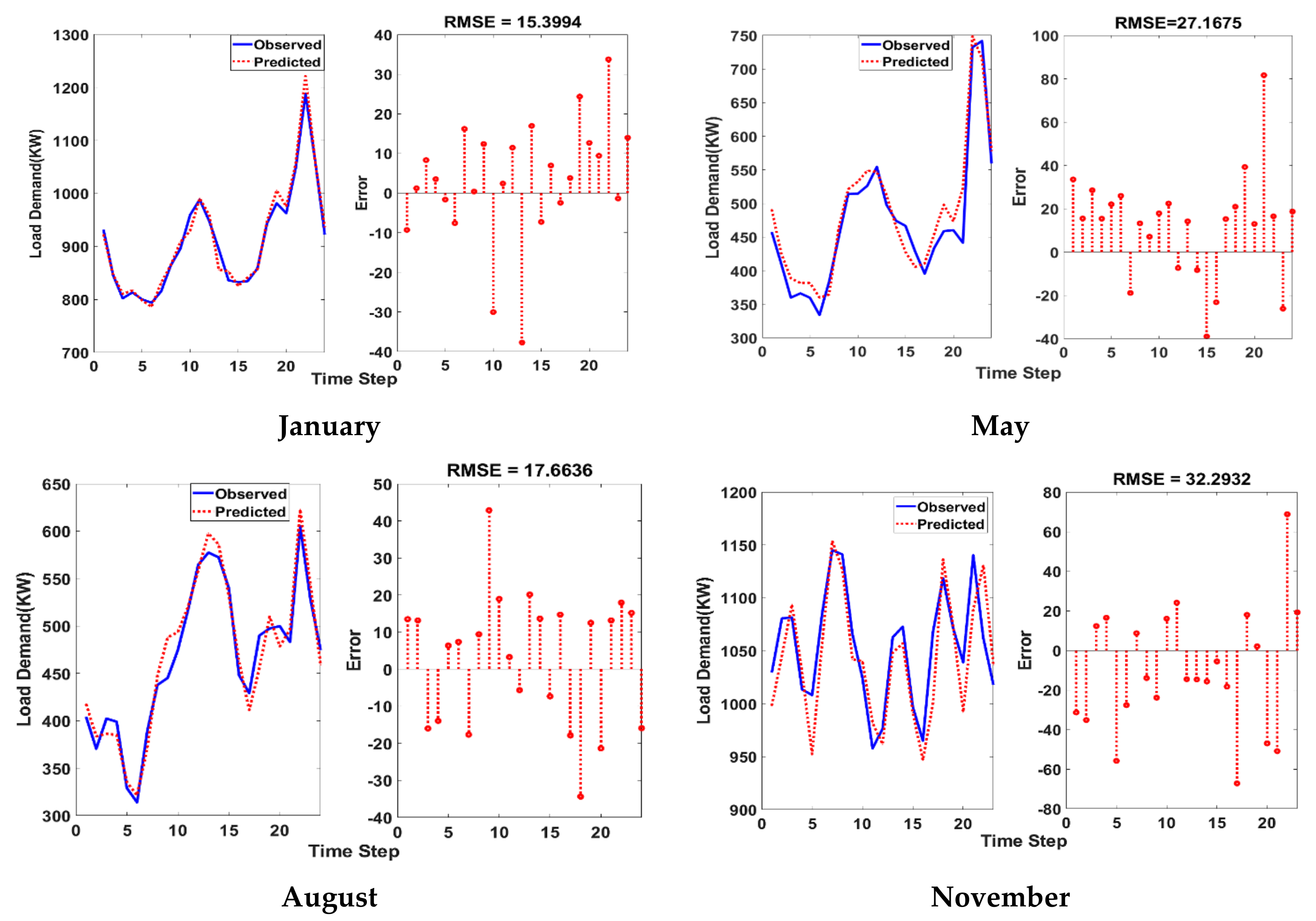RMSE indicates the deviation between the predicted value and the measured value, and it is a measure of the forecasting error [20]. The PV generation and load demand are predicted for the last day in each month of the year. Before training or testing a neural network, the training and testing data must go through a series of pre-processing steps. Normalization was applied here as the pre-processing method, which reduces the effect of different scaling of the collected data, including interpolating any missing data points and organizing the data (historical PV generation and load demand) in a chronological form [21]. The normalized data are then used as an input to the LSTM network. The initial predicted PV output power and load demand for the last day of January, May, August and November are shown in Figure 3 and Figure 4 respectively, with the RMSE indicating the accuracy of the predictions. To forecast the values of future time steps of the sequence, the training sequence with values shifted by one time step is specified as the response. This means that at each time step of the input sequence, the LSTM network learns to predict the value of the next time step. To predict the next time step, the previous prediction is used as an input to the function [22].

3. Receding Horizon Control

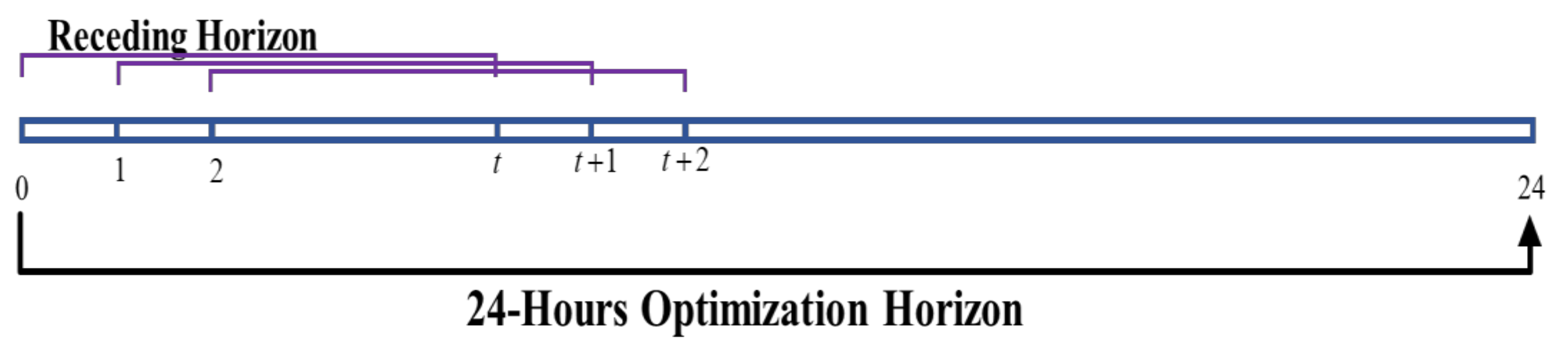
The RH strategy is a concept adopted from model predictive control (MPC), which operates by using online model-based optimization to determine the current control action [23]. It is a general-purpose control scheme that involves repeatedly solving a constrained optimization problem, using predictions of future generation and demand over a moving time horizon to choose the control action. The RH control handles constraints, such as limits on control variables, directly and naturally, and generates precisely calculated control actions, respecting the constraints. The basic RH policy is very simple. At time t, we consider an interval extending T steps into the future: t, t + 1, …, t + T, as shown in Figure 5. We then carry out several steps. For power system scheduling problems with high dependency on the forecasted values of renewable energy productions and demand, this method has been found to effectively correct errors in the prediction of renewable energy generation and load in future iterations [24]. At each hour, the economic dispatch of the battery is obtained using 24 h data of predicted future renewable energy production and demand using the LSTM network, as explained in Section 2.2. The optimization outputs are 24 h of dispatch commands, as summarized using the matrix in (22) as:

$$\left[\begin{array}{lllll}{\mathrm{P}}_{\mathrm{g}}^{\mathrm{d}}\left(1\right)& {\mathrm{P}}_{\mathrm{g}}^{\mathrm{d}}\left(2\right)& {\mathrm{P}}_{\mathrm{g}}^{\mathrm{d}}\left(3\right)& \cdots & {\mathrm{P}}_{\mathrm{g}}^{\mathrm{d}}\left(\mathrm{T}\right)\\ {\mathrm{P}}_{\mathrm{g}}^{\mathrm{b}}\left(1\right)& {\mathrm{P}}_{\mathrm{g}}^{\mathrm{b}}\left(2\right)& {\mathrm{P}}_{\mathrm{g}}^{\mathrm{b}}\left(3\right)& \cdots & {\mathrm{P}}_{\mathrm{g}}^{\mathrm{b}}\left(\mathrm{T}\right)\\ {\mathrm{P}}_{\mathrm{p}\mathrm{v}}^{\mathrm{d}}\left(1\right)& {\mathrm{P}}_{\mathrm{p}\mathrm{v}}^{\mathrm{d}}\left(2\right)& {\mathrm{P}}_{\mathrm{p}\mathrm{v}}^{\mathrm{d}}\left(3\right)& \cdots & {\mathrm{P}}_{\mathrm{p}\mathrm{v}}^{\mathrm{d}}\left(\mathrm{T}\right)\\ {\mathrm{P}}_{\mathrm{p}\mathrm{v}}^{\mathrm{b}}\left(1\right)& {\mathrm{P}}_{\mathrm{p}\mathrm{v}}^{\mathrm{b}}\left(2\right)& {\mathrm{P}}_{\mathrm{p}\mathrm{v}}^{\mathrm{b}}\left(3\right)& \cdots & {\mathrm{P}}_{\mathrm{p}\mathrm{v}}^{\mathrm{b}}\left(\mathrm{T}\right)\end{array}\right]$$

(22)

Here, only the dispatch commands for the next hour are shown (the first column of the matrix is implemented in real-time, and the rest are discarded).

The generation and demand input data to the LSTM are updated to include that of the generation and demand at the current hour $\mathit{t}$. The LSTM is then used to predict data for the next 24 h, and the process is repeated in real-time for each time step. If the time step, $\mathsf{\Delta }\mathrm{t}$, is one hour, the algorithm is repeated $\mathrm{T}/\mathsf{\Delta }\mathrm{t}$ times, which represents the number of time steps, $\mathsf{\omega }$, for $24$ h of the day. The RH final solution is the optimal schedule of the renewable energy source and the grid power for supplying the load and charging the battery.

The RH control strategy allows for the improvement of the forecasting errors for each iteration of the economic dispatch problem, since the feasibility of economic dispatch and optimality depends on the accuracy of prediction of the renewable generation in power systems [9].

4. Simulations and Results

To solve the optimization problem, a case study was developed considering data from the Ushant Island project in France under the Intelligent Community Energy (ICE) program to test the proposed approach for the real-time operation of the microgrid energy sources [25]. The proposed energy management system simulation was performed in MATLAB with a 32 GB 64-bit operating system computer, dual core i7, 2.70–2.90 GHz. The average computational time of the simulation was about 8.89 ± 2.12 s using this computer, over 12 months. Figure 1 illustrates the Ushant Island model, which has the following parameters: 3 MW PV system, grid connection and 2400 kWh battery ESS capacity. The daily ToU electricity tariff rate is shown in

Table 3. Daily time of use (ToU) electricity tariff.

Time of Day	Hour	Price
Off-peak time	22:00–5:00	0.05 £/kWh
Mid-peak time	12:00–17:00	0.08 £/kWh
Peak time	6:00–11:00, 18:00–21:00	0.17 £/kWh

. The characteristics of the ESS, such as the capacity, the SoC limits or bounds and the initial SoC, are shown in

Table 4. Characteristics of the lead-acid battery parameters.

Battery Parameters	Typical Values
Rated depth of discharge (DOD) %	50
Maximum charging power (kW)	300
Battery charge efficiency (%)	100
Battery discharge efficiency (%)	100
Maximum state of charge (%)	100
Nominal battery capacity at 100% SoC (kWh)	2400

.

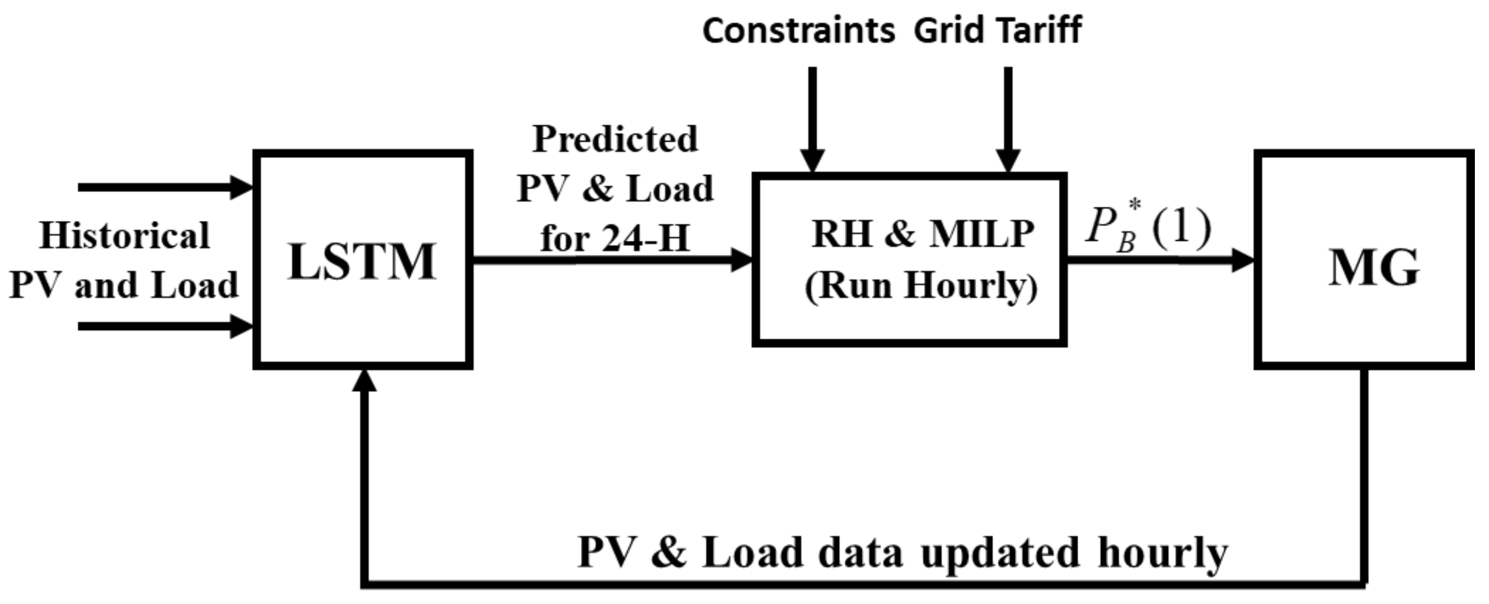
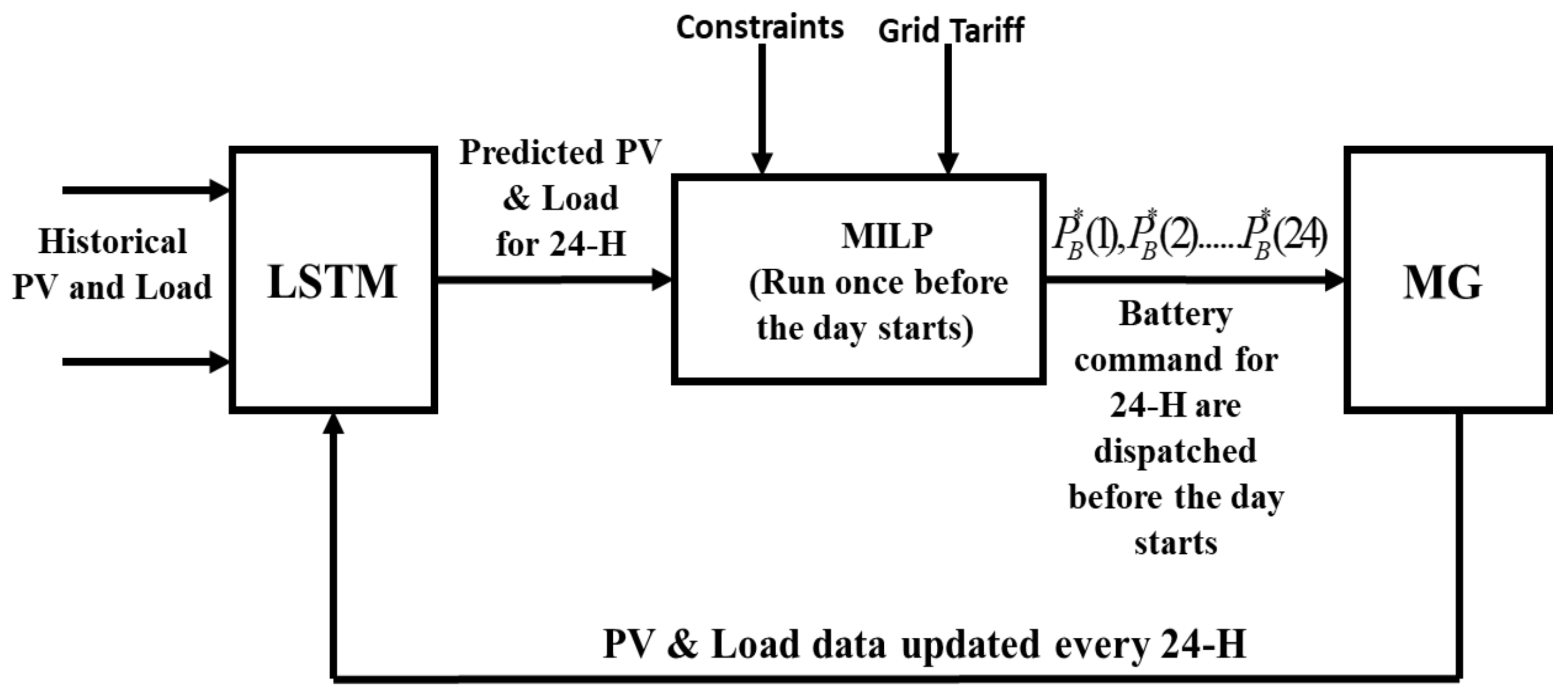
To evaluate the proposed real-time energy management of the microgrid, the simulation was carried out considering two scenarios. For the first scenario, as seen in the EMS flow model in Figure 6, the optimization is performed in real-time considering the RH technique using the real-time and predicted data simultaneously, with the real-time data used to update the input of the LSTM. The optimal daily operating cost for the 24 h horizon is recorded, while in the second scenario, as seen in Figure 7 it considers a day-ahead offline optimization using predicted data only, the ESS command is applied online with real data and the optimal daily operating cost is recorded.

The available historical data were utilized on a monthly basis by predicting the PV generation and load demand of the last day of every month. The BESS operation starts from its minimum SoC of 50%, with a maximum charging/discharging power of 300 kW.

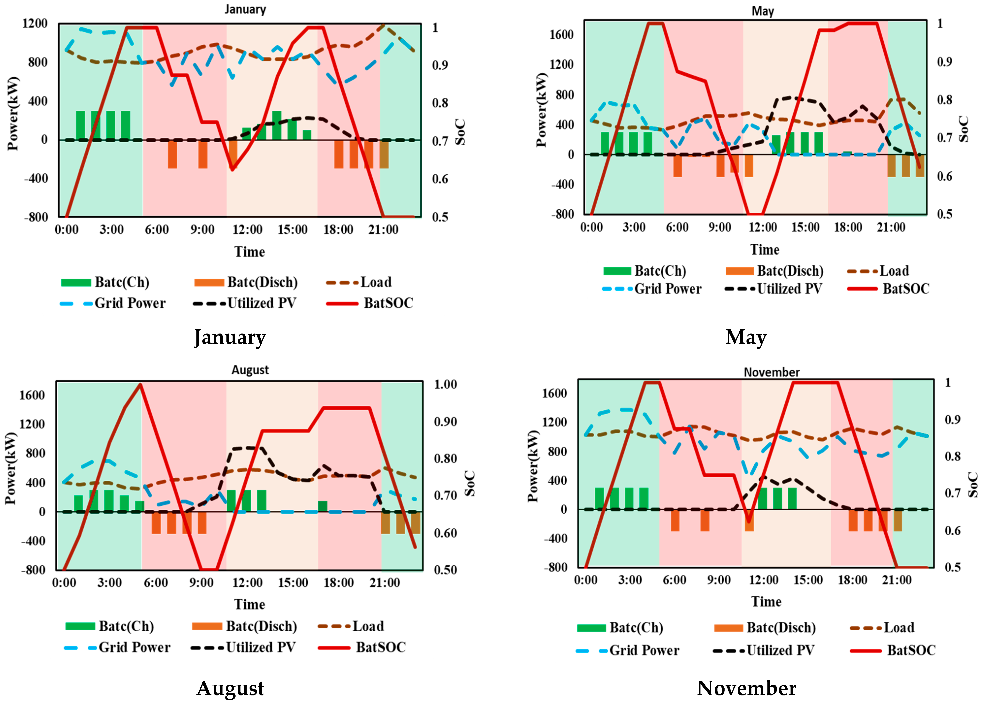
The results of the simulations for the microgrid dispatch are shown in Figure 8 when the battery charge/discharge cycle was limited to two for January, May, August and November, representing the four seasons of the year, with background colors representing the ToU tariff regions. Since the battery charge/discharge cycle is limited to two using (15)–(19), the battery starts charging at the beginning of the day when the ToU tariff is at its lowest rate (the green region), discharges when the ToU tariff is at its highest rate (the red region) and starts charging again when PV power becomes available or during the mid-peak ToU tariff (pink region), and finally discharges during the second peak of the ToU tariff. This charge/discharge pattern of the battery is consistent throughout the year and makes it easy to calculate the life of the battery ESS based on the standard lifecycle vs. the depth of discharge (DOD) curve of batteries.

A day-ahead schedule based on an offline optimization was performed with the predicted PV power and load demand for the second scenario using the MILP optimization approach. The MILP module, as shown on the EMS flow model in Figure 7, calculates the set-points for the dispatchable resources 24 h ahead based on predicted resources. The grid and the ESS are the dispatchable energy resources, which means the power output can be controlled while the PV system and the load demand are varying resources or non-dispatchable resources. The ESS command obtained from the offline day-ahead optimization was implemented in real-time on real data, as shown in Figure 7. The daily operating cost for the 24 h horizon was calculated. To evaluate the effectiveness of the proposed approach, the simulations were performed for the last day of every month, the monthly historical data were trained using the LSTM network and the last day of the month was predicted. Both scenarios were tested every month, and the daily optimal operating cost was compared against a benchmark in which the forecasted data are the same as the real data. This is a non-practical situation, but it will help us to evaluate the effectiveness of the two scenarios. 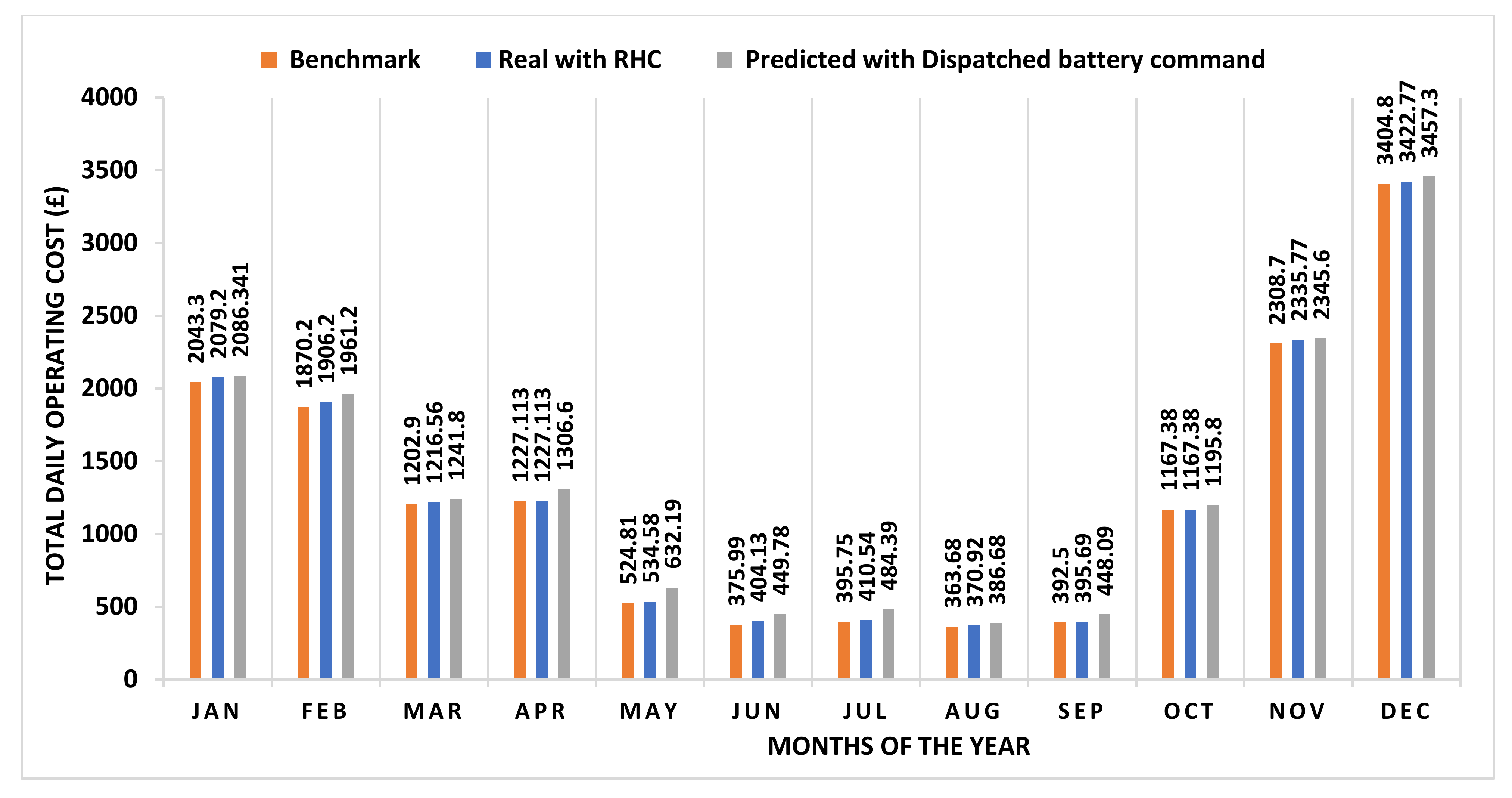Figure 9 shows the daily optimal operating cost of the microgrid for the last day of every month of the year, for the benchmark, the real-time with RHC and the offline optimization using predicted data. The simulation results show that the operating cost of the proposed real-time strategy outperformed the offline optimization strategy by 3.3%. The details of the total percentage difference between the two scenarios and how close they were to the benchmark are shown in

Table 5. Optimal cost comparison with average % difference between the two scenarios.

Months	Optimal Cost (£) (Benchmark)	Optimal Cost (£) (Online Optimization)	Optimal Cost (£) (Offline Optimization)	% Difference between the Two Scenarios
Jan	2043.30	2079.20	2086.30	0.342
Feb	1870.20	1906.20	1961.20	2.804
Mar	1202.90	1216.56	1241.80	2.033
Apr	1227.11	1227.11	1306.60	6.083
May	524.81	534.58	632.19	15.440
Jun	375.99	404.13	449.78	10.149
Jul	395.75	410.54	484.39	15.246
Aug	363.68	370.92	386.68	4.076
Sep	392.50	395.69	448.09	11.694
Oct	1167.38	1167.38	1195.80	2.376
Nov	2308.70	2335.77	2345.60	0.419
Dec	3404.80	3422.77	3457.30	0.998
Total Cost	15,277.123	15,470.853	15,995.771
% Closeness to the benchmark		1.252	4.493
Total Cost % Difference B/W the Two Scenarios				3.3

.

5. Conclusions

This paper presented an EMS to minimize the daily operating cost and control the charge/discharge cycle of ESS in a grid-tied microgrid, while guaranteeing the security of supply and respecting imposed constraints. The optimality of this approach was evaluated based on the daily operating cost of energy. Furthermore, the result from simulation studies carried out on the two scenarios considering different sets of data throughout the year shows that the online optimization adopting the LSTM-MILP-RH (online) control strategy was more effective in terms of reducing the daily operating cost when compared to the LSTM-MILP (offline) optimization approach, with the benchmark daily operating cost set as a reference. The approach is general enough to be used with different ToU tariff models and could be applied to commercial, residential and standalone microgrids.

Finally, since ESS degradation depends largely on the charging/discharging cycles, this approach guarantees a longer life for the ESS as the utilization of the ESS charging/discharging cycle limiting constraint is implemented in both scenarios. In this case, the charging/discharging cycle has been limited to two cycles.

Further research needs to be carried out in sensitivity analysis, distributed demand side management, considering different ToU tariffs (i.e., UK economy 7, UK economy 10 and UK standard tariff), to observe the effect of the ToU tariff on the battery charge/discharge cycle limits and how a change in the battery charge/discharge cycle limit will affect the daily operating cost of the microgrid.