DSO Strategies Proposal for the LV Grid of the Future

Abstract

A significant challenge for the DSO (Distribution System Operator) will be to choose the optimum strategy for flexibility service in the LV area with high RES (renewable energy sources) penetration. To this end, a representative LV grid operated in Poland was selected for analysis. Three research scenarios with RES generation were presented in the range of 1–8 kW for the power factor from 0.9 to 1. The grid PV capacity was determined for four load profiles. Based on this factor, optimum RES volume management service types were determined. Under the flexibility service, the proposed power conversion services and active RES operations for DSO were proposed. The research was conducted using the Matlab and PowerWorld Simulator environment. Optimum active power values were obtained for the RES generation function for single and dual operation systems of the power conversion system. In future, the knowledge in the field of grid capacity will enable the DSO to increase the operating efficiency of the LV grid. It will enable the optimum use of the RES generation maximisation function and proper strategy selection. It will improve the energy efficiency of the power input through the MV/LV node.

1. Introduction

The European Union strategy presented in the European Green Deal aims at reducing greenhouse gas emissions by at least 55% by 2030 [1]. The set target will be attained among other things by installing renewable energy sources, while improving the energy efficiency. The direction to de-carbonise the power generation sector has already been accepted by the member states, including Poland. One of the main premises of the transformation process is action intended to protect the planet and human health. The validity of the assumed transformation path is confirmed by section VI of the IPCC report (AR6) [2], which indicates that global warming of 1.5–2 deg C/F can be stopped by quick greenhouse gas reduction.

The commonly observed mega-trend towards the development of prosumer power generation in Poland is confirmed by the statistics in the reports presented by the President of Energy Regulatory Office [3], who point to the significant dynamics of the year-to-year increase in new installations. The dynamics of the increase in prosumer microinstallations was approximately 191% in the period of 2018/2019 and approximately 202% in the period of 2019/2020. Due to the availability of subsidies and financial support for such projects, territorial units work with the residents to de-carbonise the urban and suburban sections of the LV grid. The electricity supply and consumption balance for end consumers changes locally.

At the national level, Poland’s energy policy until 2040 predicts a fivefold increase in the number of prosumers by 2030, relative to the current condition. In addition, the number of energy-sustainable areas will increase at the local level [4]. It is predicted that microgrids will be formed based on separated sections of the LV grid. The power and electrical energy settlement for end consumers will be shifted to local balance areas as the local dispersed generation capacity increases.

It should be noted that the photovoltaic panel technology changes at the same time. At present, manufacturers are introducing to the market a new type of panel in bifacial technology [5,6,7], with higher capacity levels (500–670 kWp) than previous types, defined as ultra-high power modules. This will provide the prosumers with higher generation capacities, often exceeding their momentary power requirements.

The process of power generation sector transformation through dispersed power generation changes the operating characteristics of the LV grid [8,9], to which these sources are connected. This phenomenon has at least two new contexts. The first context is the technical adjustment of the LV grid and the second context is the current balancing of the demand and the supply according to the established quality of service parameters. The European Commission has identified the need to manage these contexts. It defined the mitigation tool as energy grid flexibility and addressed it in art. 32 of chapter IV of Directive 944/2019 [10]. This enabled the DSO to apply a freely selected strategy (demand size response, storage system, etc.), depending on the context of the LV grid operation.

Considering the above-listed factors changing the existent LV grid operation, this research was motivated by the need to develop and describe the possible strategies for the DSO in the area. At present, the authors of the paper point to two possible technical solutions. The first solution is centralised and consists in using power converter systems as energy storage systems (ESS) in the grid operation system on the DSO side [11,12,13,14,15], as part of the infrastructure. In this solution, there is no description of a particular location for grid connection (beginning, middle, end of the LV grid) and the number of such systems as ESS. These considerations are exclusively connected with a single specific test case. The second solution is decentralised and consists in using power conversion systems with energy storage systems at the consumer (prosumers) [16,17,18,19,20]. The use of dispersed ESS systems depends on the times of response to the service of the ESS user [21] and/or the availability of the ESS systems at the given adjustment moment [22]. At the given moment, each ESS features different parameters: Capacity, power, ramp, rate, cycle time [23]. The flexibility of this service is negligible, including the control/adjustment capacity on the side of the DSO. Therefore, the authors of this paper identified the research problem in the form of the selection of the strategy for the LB grid based on a measurable factor. The grid PV capacity indicator was selected [24,25,26] for the LV grid operating in Poland. The power flow throughput limits of the LV grid were the subject of this research and the resulting evaluation, positive or negative, is a proposal for strategy development by the DSO.

2. Materials and Methods

2.1. Research Problem

The basic assumption of the research is the absorption of the maximum output of electrical energy generation of all PV sources in the LV grid, without applying restrictions to micro-producers. The role of the DSO is to use the available grid flexibility utilities to:

• Maintain the voltage value at the individual connection points (0.9÷1.1)·U_n, as per EN 50160 [27,28].
• Reduce the impact of the energy flow towards the LV grid [8,29,30,31].
• Reduce the ML/LV transformer overload during PV generation [11,30,31,32].

The authors of the paper assumed the research hypothesis that flexibility service rating exists, connected with the prosumer and generation load profile. The rating was built on the basis of the cost index [33,34] (unit power price of the converter system, number of ESS in relation to the existing PV inverters) and effective grid regulation. The obtained results are presented in Section 4. The ultimate purpose was to provide the DSO with a proposal including effective service flexibility strategies in accordance with the process presented in Figure 1.

The light beige colour was used to mark the tasks that the DSO currently performed in the distribution service provision process. The dark brown colour was used to mark the tasks that the DSO would perform in the future [10].

2.2. Research Object

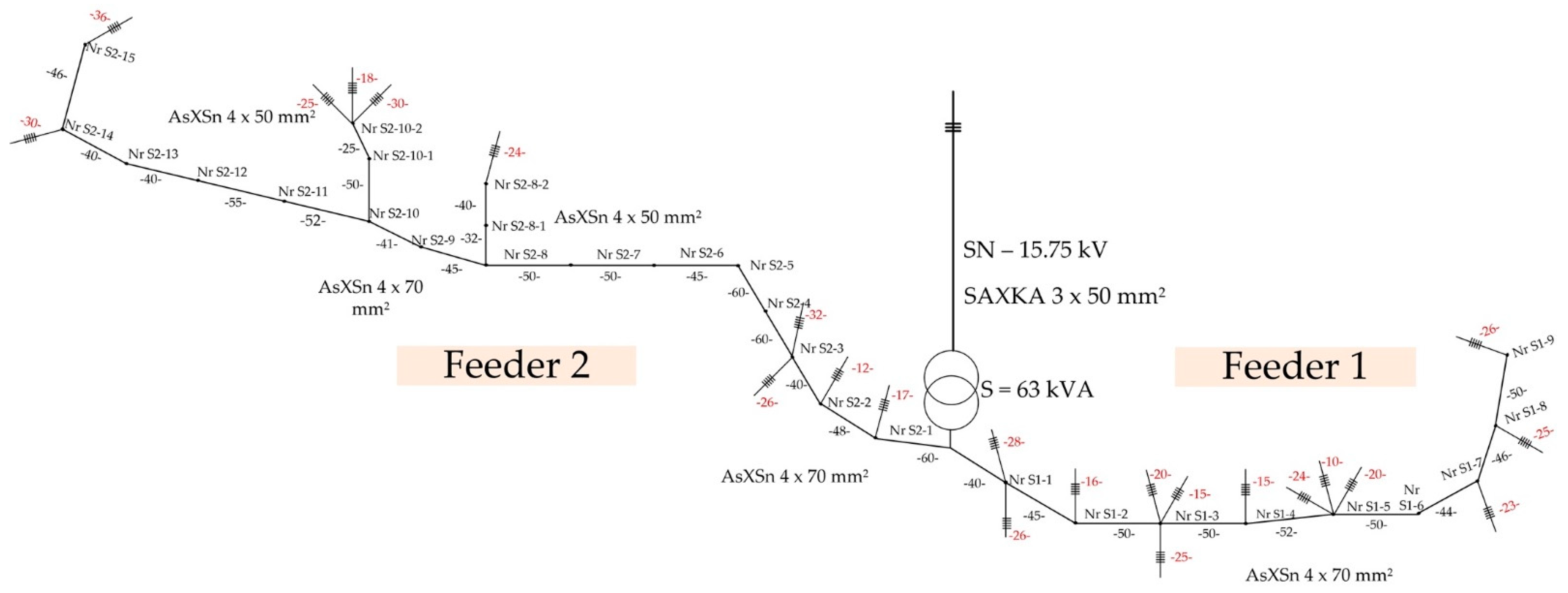
The DSO infrastructure of the LV grid selected for research purposes was typical of suburban areas of agglomerations, to which new dispersed energy sources were connected systematically. The LV grid is radial and overhead, with two feeders (F1 and F2). The bus is made using a wire with a section of 70 mm²; this results directly from the DSO standard in Poland [35]. The LV grid diagram is presented in Figure 2. The LV grid is connected with 23 consumer/prosumers with the connection power of 11 kW. Figure 2 shows the distances of the individual sections of the F1 and F2 bus (unit: Meter, e.g., −45—between the power poles Nr S1-1 and Nr S1-2).

The technical specifications of the analysed grid were specified in

Table 1. Technical specifications of the overhead line [36].

AsXSn LV	50 mm2	70 mm2
R [Ω/km]	0.641	0.443
X [Ω/km]	0.085	0.083
SAXKA MV	50 mm2
R [Ω/km]	0.641	-
X [Ω/km]	0.144	-

,

Table 2. Technical specifications of the transformer.

Power Rate	63 kVA
Voltage rate MV/LV	15.75/0.4 kV
Winding configuration	Dyn5
No load loss	0.81 kW
Load loss	1.2 kW
Impedance	4.5%

and

Table 3. Distances between the MV/LV transformer and the connection points (only data per consumer/connection point).

Connector Number	Feeder 1 [km] (Name)	Feeder 2 [km] (Name)
1	0.066 (1.01)	0.077 (2.01)
2	0.068 (1.02)	0.120 (2.02)
3	0.10 (1.03)	0.174 (2.03)
4	0.150 (1.04)	0.18 (2.04)
5	0.155 (1.05)	0.509 (2.05)
6	0.160 (1.06)	0.592 (2.06)
7	0.247 (1.07)	0.599 (2.07)
8	0.257 (1.08)	0.604 (2.08)
9	0.261 (1.09)	0.716 (2.09)
10	0.262 (1.10)	0.768 (2.10)
11	0.354 (1.11)	-
12	0.402 (1.12)	-
13	0.453 (1.13)	-

The total length of LV line for feeder 1 = 0.427 km, for feeder 2 = 0.732 km.

. The technical specifications were extracted from the LV line design and supplemented with catalogue specifications.

2.3. Boundary Conditions for Simulations

Research works were conducted based on specifications of the actual LV grid in Central Poland (Table 1, Table 2 and Table 3). To this end, the Matlab environment was used, integrated through dedicated scripts with the PowerWorld Simulator environment (Figure 3). Power distribution for the given condition, for each connection point, was calculated in accordance with the following formula (Equations (1) and (2)) [22,37].

$$P_k\left(V_k,V_j,{\theta }_k,{\theta }_j\right)={{\displaystyle \sum }}_{j=1}^N\left|V_k\right|\left|V_j\right|(G_{kj}\cos ({\theta }_{kj})+B_{kj}\sin ({\theta }_{kj}))$$

(1)

$$Q_k\left(V_k,V_j,{\theta }_k,{\theta }_j\right)={{\displaystyle \sum }}_{j=1}^N\left|V_k\right|\left|V_j\right|(G_{kj}\sin ({\theta }_{kj})-B_{kj}\cos ({\theta }_{kj}))$$

(2)

where:

P_k—active power at bus k;

Q_k—reactive power at bus k;

V_k—Voltage magnitude at bus k;

V_j—Voltage magnitude at bus j;

G_kj—Mutual conductance between buses k and j;

B_kj—Mutual susceptance between buses k and j;

θ_kj—Voltage angle difference between buses k and j;

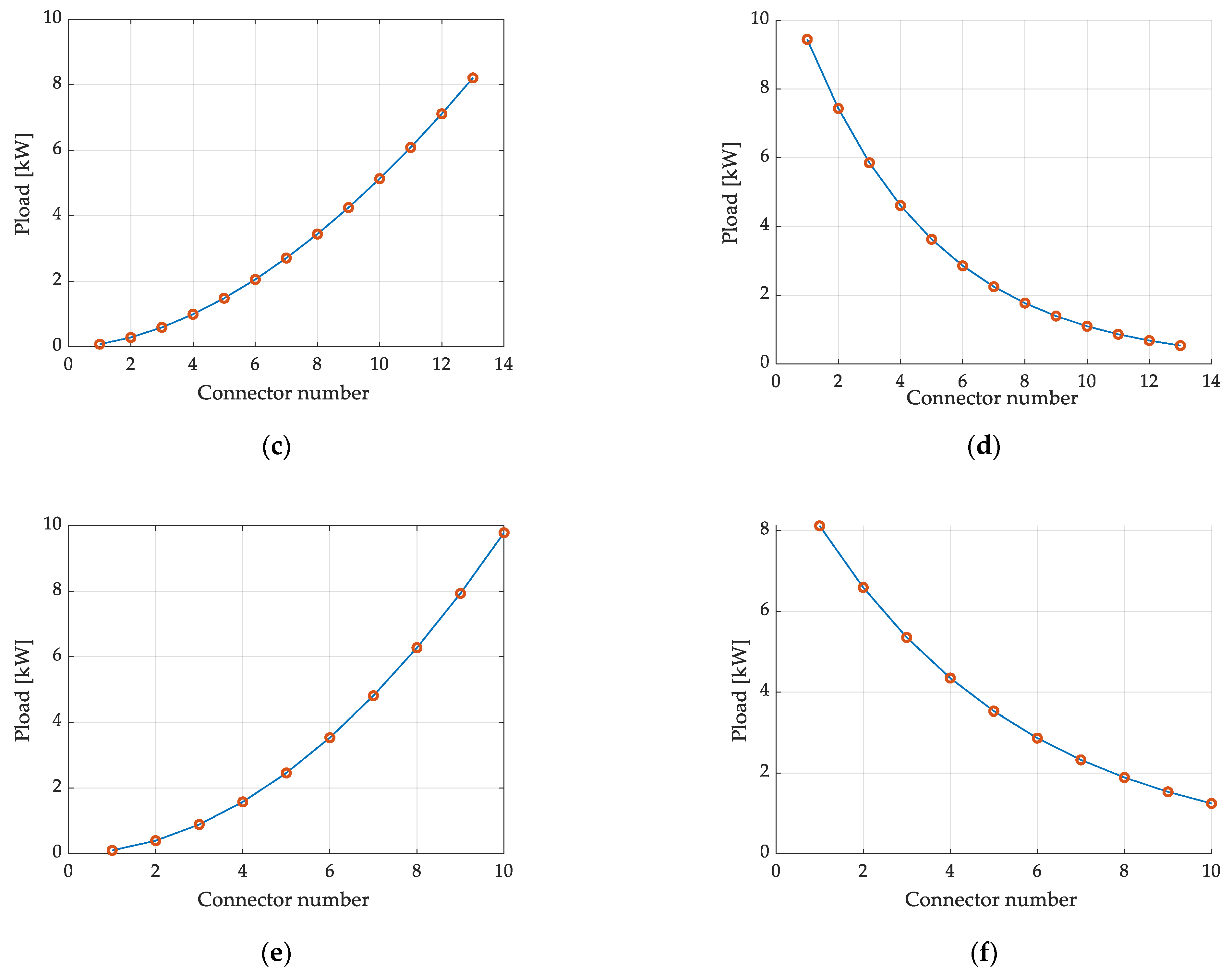
One of the most important components for the development of proper evaluation of LV grid operation with a large number of PV generators is proper selection of the P_l load model by the consumer/prosumers. The consumer profiles used in simulation are selected to include the broadest possible range of cases possible under the given conditions, the most extreme for the LV grid operation [38]. In addition, P_l has a direct impact on the LV grid operation, balancing or not the current/present generation profile—P_gc. The four selected profiles P_l are presented in Table 4.

Table 4. Load profiles used in power distribution simulations.

Profile Pl	Name	Feeder 1	Feeder 2
1. Simultaneity factor for peak power demand in accordance with the Polish standard SEP-E-002, Figure 4a	SF	3.27 kW	3.78 kW
2. Right skewed Figure 4c,e $\mathrm{distribution} \mathrm{exponential} \mathrm{function} f\left(x\right)=a^x$	RS	${\displaystyle \sum _n^{n=13}}{P}_l=42.51 \mathrm{kW}$	${\displaystyle \sum _n^{n=10}}{P}_l=37.8 \mathrm{kW}$
3. Left skewed Figure 4d,f $\mathrm{distribution} \mathrm{exponential} \mathrm{function} f\left(x\right)=x^a$	LS	${\displaystyle \sum _n^{n=13}}{P}_l=42.51 \mathrm{kW}$	${\displaystyle \sum _n^{n=10}}{P}_l=37.8 \mathrm{kW}$
4. Random data, Figure 4b	RD	<0.5–2.5> kW	<0.5–2.5> kW

Table 4. Load profiles used in power distribution simulations.

Profile Pl	Name	Feeder 1	Feeder 2
1. Simultaneity factor for peak power demand in accordance with the Polish standard SEP-E-002, Figure 4a	SF	3.27 kW	3.78 kW
2. Right skewed Figure 4c,e $\mathrm{distribution} \mathrm{exponential} \mathrm{function} f\left(x\right)=a^x$	RS	${\displaystyle \sum _n^{n=13}}{P}_l=42.51 \mathrm{kW}$	${\displaystyle \sum _n^{n=10}}{P}_l=37.8 \mathrm{kW}$
3. Left skewed Figure 4d,f $\mathrm{distribution} \mathrm{exponential} \mathrm{function} f\left(x\right)=x^a$	LS	${\displaystyle \sum _n^{n=13}}{P}_l=42.51 \mathrm{kW}$	${\displaystyle \sum _n^{n=10}}{P}_l=37.8 \mathrm{kW}$
4. Random data, Figure 4b	RD	<0.5–2.5> kW	<0.5–2.5> kW

The generation PV profiles P_gc for Central Poland are the production hours from 9 am to 6 pm within prosumer load demand P_l, in the same time [39]. The value P_l on the side of prosumers is different for period: (A) Saturday–Sunday/holiday, (B) Monday–Friday. Generally, P_l in the LV grid is stochastic. Therefore, an attempt was made to define the boundary conditions so that they contain the largest number of solutions corresponding to the real P_l profile. The first three profiles—SF, RS, LS—correspond to period A. With this end in view, defined load with a constant value (SF) was calculated in accordance with the standard SEP-E-002 (power connection 11 kW). The other two profiles, RS and LS, are unequal loads. There are differences at the beginning and end of the circuit F1 and F2. This has been described mathematically (Table 4). The fourth profile (Table 4.4) is typical loads for period B, where the profile is developed based on small household appliances (refrigerator) and electronics in stand-by mode.

The apparent power distribution in the LV grid for each of the described profiles P_l, were simulated for P_gc in the range of 1 kW to 8 kW and tracking of 0.25 kW. Since the LV grid, despite the high R/X ratio [37], does not operate in pure resistance mode (PV power electronic system operation) [40], PV generation is simulated for the power factor (p.f.) from 0.9 to 1. The encountered voltage asymmetry in the LV grid was eliminated by the four-wire power conversion system, controlled independently for each phase [41,42]. In the research, this fact was omitted as negligible; phases F1 and F2 can be considered as technically separate and controlled independently.

2.4. Scenarios

The boundary conditions described in the previous section as components of data input for the research were framed in three research scenarios. In addition, the operating system of the LV grid (Figure 1) is supplemented with ESS operating in the grid feeding mode [43] (Figure 5).

The operation of the LV grid with ESS was controlled by the inputs P (active power) and Q (reactive power) of the power converter system (Figure 5) to achieve the objectives described in Section 2.1 (Numbers 1–3).

The first research scenario is the evaluation of the grid PV capacity for LV, the “AS IS” condition analysis. The input data values P_gc and P_l were searched for the LV grid, where the voltage requirement of 1.1 Un is not met. In addition, power flows towards MV through the transformer were checked.

The second research scenario was implemented using ESS in the operation system, Figure 6a. The analysis covered the LV grid and its operating characteristics with the boundary conditions described in Section 2.3 to define the values of P and Q for ESS. Location at one point of the grid—the MV/LV station (Figure 6a).

The third research scenario was implemented using two ESS systems: S1 and S2 in the operation system, Figure 6b. The analysis covered the LV grid and its operating characteristics with the boundary conditions described in Section 2.3 to define the values of P1, P2 and Q1, Q2 for S1 and S2 (Figure 6b). The location of the ESS in the depth of the LV grid is based on the data of scenario no. 1.

3. Results

By iterative power flow analysis in the dedicated LV grid, within the scope of three scenarios and four load profiles, the answer was obtained in the field of grid PV capacity. Developed results presented in

Table 5. Capacity Grid for four load profiles.

Capacity Grid	SF	RS	LS	RD
Feeder 1, cosf(φ) = 1.00 for PV	<8 kW	<8 kW	<8 kW	7.5 kW
Feeder 2, cosf(φ) = 1.00 for PV	7.75 kW	<8 kW	7.0 kW	5.75 kW
Feeder 1, cosf(φ) = 0.95 for PV	6.5 kW	7.25 kW	5.75 kW	5.5 kW
Feeder 2, cosf(φ) = 0.95 for PV	6.0 kW	6.75 kW	5.25 kW	4.25 kW
Feeder 1, cosf(φ) = 0.90 for PV	5.75 kW	6.25 kW	5.0 kW	4.5 kW
Feeder 2, cosf(φ) = 0.90 for PV	5.25 kW	6.0 kW	4.75 kW	4.0 kW

The values presented in Table 5 are the starting point for the regulation of power converter systems (power tracking) in accordance with the diagram in Figure 5. The obtained grid PV capacity results will also be the basis for the evaluation of the strategy selection on the DSO side. Green: Grid PV capacity values that do not require adjustment for a given load profile; red: Those cases of LV network operation that require a response from the DSO; yellow: Result values are shown for little regulation adjustment.

. Based on them, a non-linear function was developed, described in three dimensions f(x, y, z) where: x—distance from the MV/LV station (distance); y—values of PV current generation (P_gc); z—voltage at the given node (U p.u.). It should be emphasized that the results in Table 5 are the maximum values of PV power generation for which the Un = 1.1 condition is met for each node in the LV grid.

Analytical research was carried out in two ways. The first track of works was carried out in the field of searching for a grid PV capacity for one value of the maximum RES generation capacity per every node. The second course was carried out by the optimal grid PV capacity values for all nodes (different values of RES per node). Below is a mathematical model for the second track.

The purpose of the research is to maximise RES generation. Therefore, the objective function is grid PV capacity measured by the maximum generation value of P at cos(φ) = const., for which the voltage requirements for the electrical energy supply are met. For the purposes of optimisation of the objective function f(x, y, z), the equations of Karush–Kuhn–Tucker [44,45] for non-linear programming algorithms were used, following the formulae (Equations (3)–(6)) [46]:

$$\begin{array}{c}max\\ x\in {ℝ}^n\end{array}=f\left(x\right)$$

(3)

$$L\left(x,u,v\right)=f\left(x\right)+{\displaystyle \sum }_{i=1}^m{\mu }_i{g}_i\left(x\right)+{\displaystyle \sum }_{j=1}^r{\lambda }_j{h}_j\left(x\right),$$

(4)

$$-\nabla f\left(x\right)+{\displaystyle \sum }_{i=1}^m{\mu }_i\nabla g_i\left(x\right)+{\displaystyle \sum }_{j=1}^r{\lambda }_i\nabla h_j\left(x\right)=0,$$

(5)

$$\begin{array}{c}{g}_i\left(x\right)\le 0, for i=1, \dots ,m\\ h_i=0, for j=1,\dots .,r\\ {\mu }_i{g}_i\left(x\right)=0, for i=1, \dots .,m.\end{array}$$

(6)

The objective function has two limits: g_i—in the RES power range (P_gc); h_i—in the 1.1 p.U. value range for each node (U per unit).

3.1. The First Scenario

The first scenario is dedicated to the evaluation of grid PV capacity without flexibility service. It clearly indicates the limits, at which the given feeder (F1 and F2) achieves the maximum operating values. In addition, Figure 6 presents the results of optimisation of RES operation. However, Figure 5 presents the operation profile of the MV/LV transformer in this type of grid.

3.1.1. Grid PV Capacity

In Table 5, the max P_gc values obtained for each P_l profile were listed. At the same time, reactive power from the RES side was input at connection points.

3.1.2. Optimisation of the Non-Linear Function

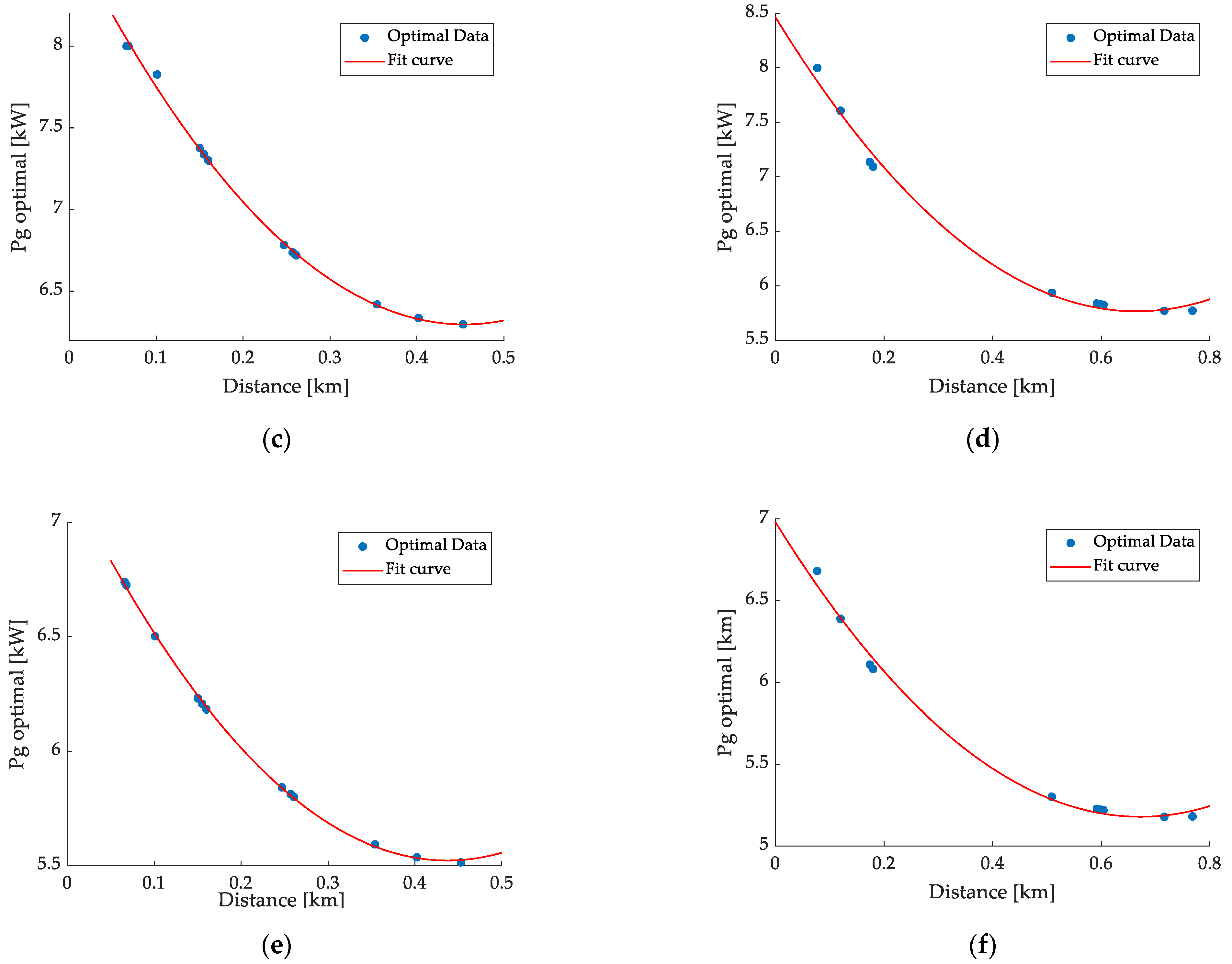
In Figure 7, only for P_l = SR (limited due to the number of possible diagrams), optimum RES generation values were presented for each connection point as a function of the distance. These are the optimum values of grid PV capacity per node. The analysis points to the limits for the individual feeders and individual nodes. This points to the potential ESS connection point in the depth of the grid, the minimum value of the function in the given distance range.

3.1.3. Operation Balance for the MV/LV Transformer

For the load profile of P_l = SR, as in the previous sub-section, power inputs through the MV/LV station were determined as a function of RES generation increase. Figure 8 shows how the power input from the MV grid to the LV grid changes the vector to LV to MV. The process is completed regardless of the type of load profile and p.f., in connection with the increase of the RES generation value (P_gc).

Therefore, the selection of transformer power at high RES penetration is important. Nominal service operation with PV requires re-selection of the transformer power or in addition requires the use of flexibility service.

3.1.4. Reactive Power during PV Generation

The requirements for PV inverters on the side of the DSO are p.f. = 1. Due to the quality of the power electronic systems used by the prosumers, deviations from this value exist. Notwithstanding, this type of operation in case of small P_l power values does not serve its purpose in terms of grid PV capacity (Table 5).

The second method is active collaboration with the prosumers for reactive power consumption from the LV grid. Reactive power could be managed by PV inverters in the p.f. range of 0.9–1. This will reduce the RES production, but at the same time it will enable the prosumer to provide service to the DSO. Below is presented the most demanding case: P_l = RD and p.f. = 0.9, the results of the described prosumer service. Figure 9 features the RMS value of the nodal voltage for the two feeders—blue, while red states restriction level for node 1.1 Un.

The conducted research proved that in this case, regardless of the load profile, and for RES generation in the range of 〈$1:8$〉 kW, there is no voltage excess at node points. This is the most effective method; however, it depends on a third party.

3.2. The Second Scenario

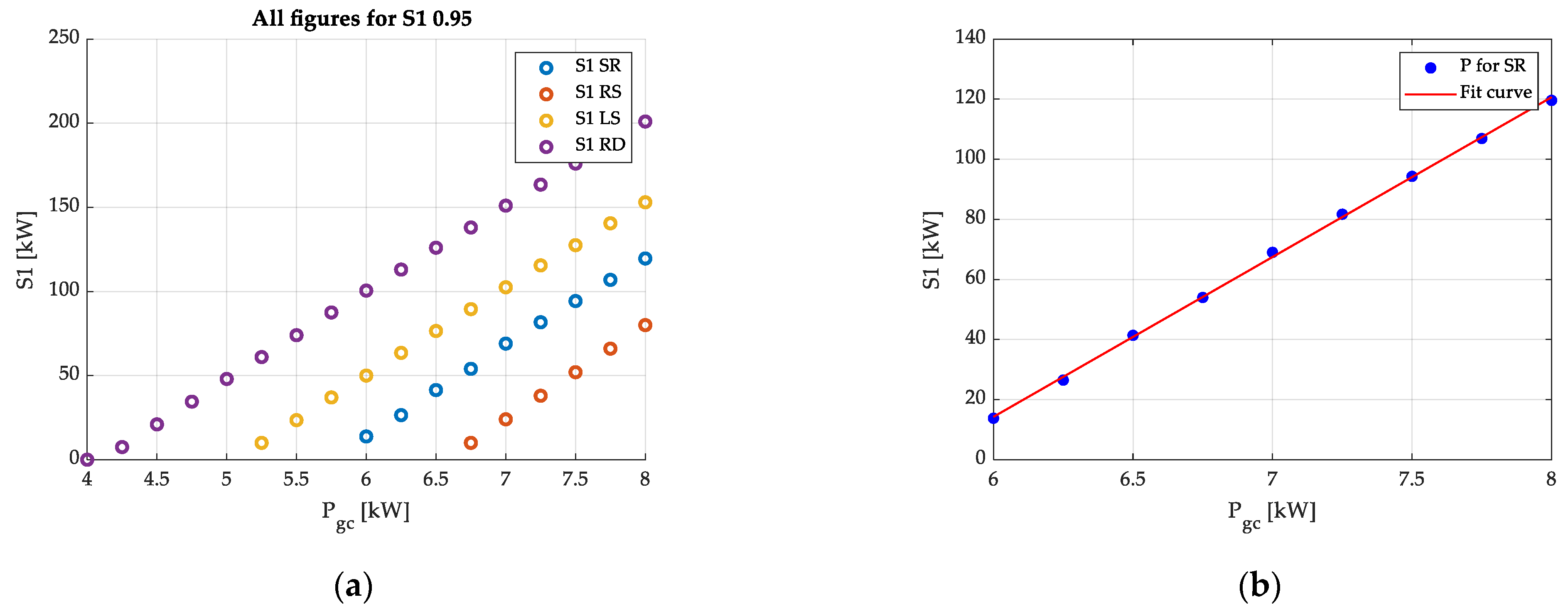
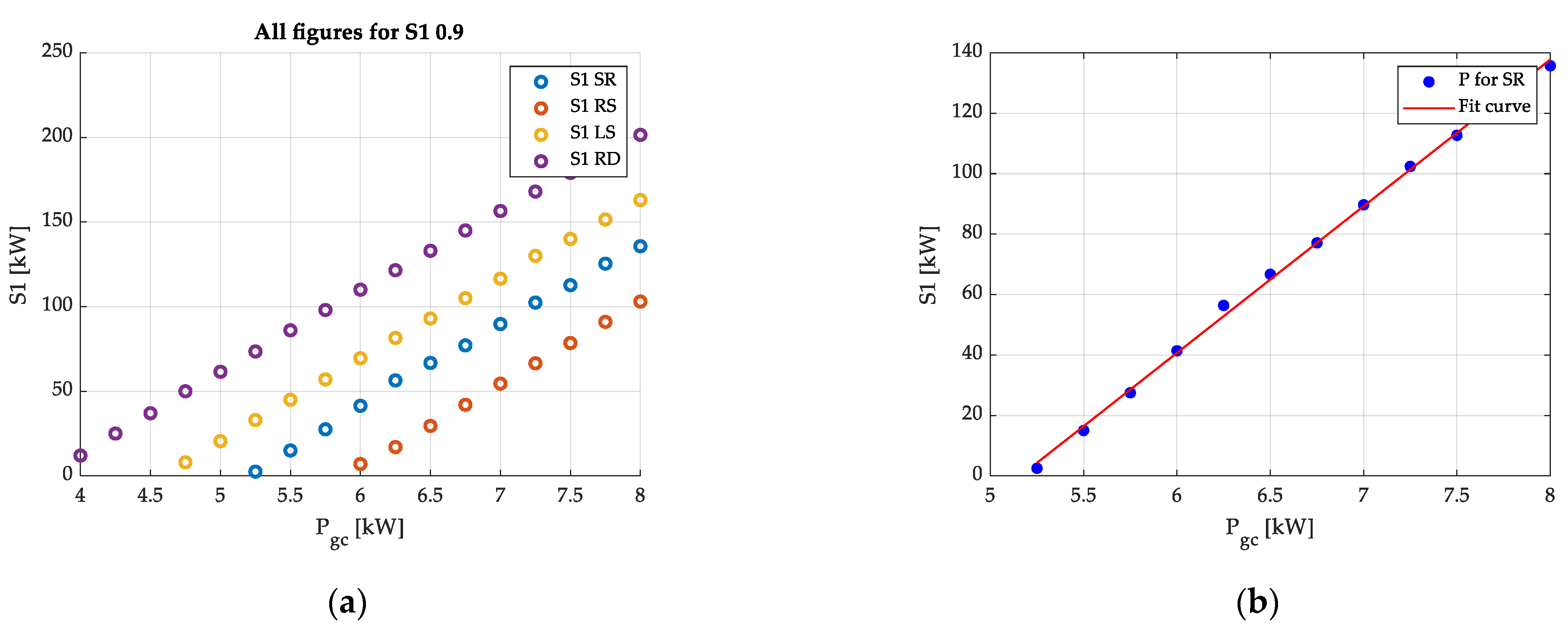
The second scenario is dedicated to the evaluation of the required capacity of the power conversion system for voltage condition adjustment at nodes. The operation system is presented in Figure 6a. The volume of data collected for S1 at the given P_l depends on the grid PV capacity (Table 5). Figure 10, Figure 11 and Figure 12 present the active power values P for S1, with identification of the function S1 = f(P_gc).

In accordance with the obtained results (Table 5), only three load profiles are subject to power input adjustment. Adjusted R-square (R²) for SR = 1 (small data volume), R² for LS = 0.9997, R² for RD = 0.999.

In accordance with the obtained results (Table 5), four load profiles are subject to power input adjustment. R² for SR = 0.9993, R² for PS = 1, R² for LS = 0.9998, R² for RD = 0.9996.

In accordance with the obtained results (Table 5), four load profiles are subject to power input adjustment. R² for SR = 0.998, R² for PS = 0.9996, R² for LS = 0.9997, R² for RD = 0.9997. The application of only S1 for operation adjustment only is to maintain the voltage conditions with active power from 2.5 kW to 201.5 kW.

3.3. The Third Scenario

The third scenario is dedicated to the evaluation of the required capacity for two power conversion systems for voltage condition adjustment at nodes, independent of F1 and F2. The operation system is presented in Figure 6b. Two ESS systems: S1 and S2 are connected in the depth of the LV grid. For F1, it is the node No. S2_10_2 (Figure 2); for F2 it is the node No. S1_7 (Figure 2). The volume of data collected for S1 at the given load profile depends on the grid PV capacity (Table 5). Due to the collected data volume, the results are presented in tables (

Table 6. Results for S1 and S2, p.f. = 1.

Load Profile/Pgc (kW)	5.75	6.0	6.25	6.5	6.75	7.0	7.25	7.5	7.75	8.0
SR
S1 (kW)	-	-	-	-	-	-	-	-	0	0
S2 (kW)	-	-	-	-	-	-	-	-	0.5	2.5
LS
S1 (kW)	-	-	-	-	-	0	0	0	0	0
S2 (kW)	-	-	-	-	-	1.5	4.0	6.0	8.5	11.0
RD
S1 (kW)	0	0	0	0	0	0	0	0	0	2.0
S2 (kW)	1.5	4.0	6.0	8.0	10.0	12.5	14.5	16.5	19.0	21.0

R² for SR S2 = 1 (small data volume), R² for LS S2 = 0.9982; R² for RD S1 = 0.9997; RD S2 = 0.9994. On average, approximately 40% smaller active power is required to control the LV grid if two, not one, ESS systems are used. In extreme cases (P_gc = 8 kW), even approximately 90% smaller.

,

Table 7. Results for S1 and S2, p.f. = 0.95.

Load Profile/Pgc (kW)	5.75	6.0	6.25	6.5	6.75	7.0	7.25	7.5	7.75	8.0
SR
S1 (kW)	-	0	0	0.5	3.0	5.0	7.5	10.0	12.0	14.5
S2 (kW)	-	2.5	5.5	7.0	9.5	12.0	13.5	15.5	18.0	20.0
RS     S1 (kW)     S2 (kW)	- -	- -	- -	- -	0 1.0	0 4.0	0.5 6.5	3.5 8.5	6.0 11.0	8.5 13.0
LS
S1 (kW)	0	2.0	4.5	7.0	9.0	11.5	14.0	16.5	18.5	21
S2 (kW)	6.5	9.0	11.0	13.0	15.0	17.5	19.5	21.5	23.5	25.5
RD
S1 (kW)	3.5	5.5	8.0	10.5	13.0	15.5	17.5	20.0	22.5	24.5
S2 (kW)	15.5	18.0	19.5	21.5	23.5	25.5	27.5	30.0	32.0	34.0

R² for SR S1 = 0.9991, S2 = 0.9967; R² for LS S1 = 0.9995, S2= 0.9994; R² for PS S1 = 0.9968, S2 = 0.9762; R² for RD S1 = 0.9995, RD S2 = 0.9972.

and

Table 8. Results for S1 and S2, p.f. = 0.9.

Load Profile/Pgc (kW)	5.75	6.0	6.25	6.5	6.75	7.0	7.25	7.5	7.75	8.0
SR
S1 (kW)	1.5	3.5	6.0	8.5	10.5	13.5	16.0	18.5	20.5	23.0
S2 (kW)	6.0	8.5	10.0	12.5	14.5	16.5	18.5	20.5	23.0	25.0
RS
S1 (kW)	-	0.0	1.0	3.5	6.0	9.0	11.5	14.5	17.5	20.5
S2 (kW)	-	1.5	4.0	6.0	8.0	10.5	12.5	14.5	17.0	19.5
LS
S1 (kW)	7.0	9.5	11.5	14.0	16.5	19.0	21.5	24.0	26.0	28.5
S2 (kW)	11.5	13.5	15.5	17.5	19.5	22.0	24.0	26.0	28.0	30.5
RD
S1 (kW)	10.0	12.5	15.0	17.5	20.0	22.0	24.5	27.5	30.0	33.5
S2 (kW)	19.0	21.5	23.5	25.5	27.5	30.0	31.5	33.0	36.0	37.5

R² for SR S1 = 0.9989, S2 = 0.986; R² for LS S1 = 0.9994, S2= 0.9988; R² for PS S1 = 0.9986, S2 = 0.9989; R² for RD S1 = 0.9985, RD S2 = 0.9985.

).

4. Discussion

The collected simulation data clearly indicate that the consumer load profile with simultaneous RES generation has a direct impact on the grid PV capacity (Table 5). Based on the completed mathematical power flow simulation in the LV grid, in different research scenarios, it should be ascertained that the control (maintenance of the voltage value of 1.1 Un) and efficient balance optimisation (Figure 5) of the grid are possible. The research indicates that there is no single method of flexibility service. Proper selection of the method depends on the effective grid regulation and profitability (capex and/or opex) and the day of the week (confirmed hypothesis—Section 2.1). These above-mentioned items will build a method rating for a given area of the grid.

Table 9. Proposed flexibility service rating.

Type of Flexibility Service	SF	RS	LS	RD
PV inverter Inverter parameters power factor = 1, Additional requirements in Networks Codes DSO.	+	+	+/−	−
PV inverter Reactive power consumption,	+	+	+	+
One ESS system central installation, connected with main bus	+/−	+	-	−
Two ESS systems Storage systems installed in the depth of the grid	+	+	+	+/−
DSR signals calling for an increase in power consumption	−	+/−	+	+
Hybrid bundling services	+/−	+/−	+	+

lists flexibility service proposals according to the load profile type (Table 4). It also represents a method rating using a colour and mark (+, −, +/−). Green is used to mark the types of service that provides technical efficiency at the lowest cost per service. Yellow is used to mark the services that do not provide the full range of LV grid adjustment and/or that may have a high cost per service. Red is used to mark the services that do not provide LV grid adjustment and/or are too expensive [47,48].

In addition, the research indicates a quasi-linear (laboratory confirmation required) relationship between the P and jQ of RES generation, and the P and jQ of the power conversion system S1 and/or S2. There is an error connected with non-linearity, measured by the indicator of function alignment with measurement data, adjusted R-square statistic, which is close to 1 (descriptions under Table 6, Table 7 and Table 8). The error results only from the precision of ESS control by power increase in 0.25 kW increments [49]. The simplest and cheapest service method is the maintenance of the p.f. close to 1 by RES or reactive power consumption by the inverter [50,51]. The developed results (data) will be used in the future to build machine learning for the purposes of power and voltage regulation in the LV grid [52,53,54].

5. Conclusions

There is still need for research works on bridging the gap between power generation based on end consumer supplied from central generation units and power generation based on local RES. The assumed research hypothesis (section research problem) was confirmed by the results obtained in dedicated scenarios (Table 5, Table 6, Table 7 and Table 8, Figure 7, Figure 8, Figure 9, Figure 10, Figure 11 and Figure 12). The basic task of the future DSO is to prepare the bus LV grid—the minimum section of 70 mm²—for the mega-process that is RES growth in the grid. In addition, the accumulation of knowledge of the load profile and generation is necessary for the development of grid PV capacity, as well as future strategies of dedicated services.

Proper selection of the MV/LV transformer with ESS remains an extremely important issue. Even constant PV generation at the level of 3.5 kW in the investigated LV grid resulted in the change of the power flow direction. The services proposed in Table 9 directly contribute to the transformer load balance, but full coverage of the power flow towards MV will only be possible in connection with ESS.

References

- European Commission. Available online: https://ec.europa.eu/info/strategy/priorities-2019-2024/european-green-deal/delivering-european-green-deal_en#transforming-our-economy-and-societies (accessed on 30 September 2021).
- IPCC Home. Available online: https://www.ipcc.ch/report/ar6/wg1/ (accessed on 30 September 2021).
- Biuletyn Informacji Publicznej Urząd Regulacji Energetyki. Available online: https://bip.ure.gov.pl/bip/o-urzedzie/zadania-prezesa-ure/raport-oze-art-6a-ustaw/3793,Raport-dotyczacy-energii-elektrycznej-wytworzonej-z-OZE-w-mikroinstalacji-i-wpro.html (accessed on 30 September 2021).
- Ministerstwo Klimatu i Środowiska. Available online: https://www.gov.pl/web/klimat/polityka-energetyczna-polski-do-2040-r-przyjeta-przez-rade-ministrow (accessed on 30 September 2021).
- Olczak, P.; Olek, M.; Matuszewska, D.; Dyczko, A.; Mania, T. Monofacial and Bifacial Micro PV Installation as Element of Energy Transition—The Case of Poland. Energies 2021, 14, 499. [Google Scholar] [CrossRef]
- Kopecek, R.; Libal, J. Bifacial Photovoltaics 2021: Status, Opportunities and Challenges. Energies 2021, 14, 2076. [Google Scholar] [CrossRef]
- Jang, J.; Pfreundt, A.; Mittag, M.; Lee, K. Performance Analysis of Bifacial PV Modules with Transparent Mesh Backsheet. Energies 2021, 14, 1399. [Google Scholar] [CrossRef]
- Pereira, C.O.; Cunha, V.C.; Riciiradi, T.R.; Riboldi, V.B.; Tuo, J. Pre-Installation Studies of a BESS in a Real LV Network with High PV Penetration. In Proceedings of the 2019 IEEE PES Innovative Smart Grid Technologies Conference—Latin America (ISGT Latin America), Gramado City, Brazil, 15–18 September 2019. [Google Scholar]
- Bangash, K.N.; Farrag, M.E.A.; Osman, A.H. Manage Reverse Power Flow and Fault Current Level in LV Network with High Penetration of Small-Scale Solar and Wind Power Generation. In Proceedings of the 2018 53rd International Universities Power Engineering Conference (UPEC), Glasgow, Scotland, 4–7 September 2018. [Google Scholar]
- EUR-Lex. Available online: https://eur-lex.europa.eu/legal-content/PL/ALL/?uri=CELEX%3A32019L0944 (accessed on 30 September 2021).
- Gao, X.; Sossan, F.; Christakou, K.; Paolone, M.; Liserre, M. Concurrent Voltage Control and Dispatch of Active Distribution Networks by means of Smart Transformer and Storage. IEEE Trans. Ind. Electron. 2018, 65, 6657–6666. [Google Scholar] [CrossRef] [Green Version]
- Zarrilli, D.; Giannitrapani, A.; Paoletti, S.; Vicino, A. Energy Storage Operation for Voltage Control in Distribution Networks: A Receding Horizon Approach. IEEE Trans. Control Syst. Technol. 2018, 26, 599–609. [Google Scholar] [CrossRef]
- Zupancic, J.; Lakic, E.; Medved, T.; Gubina, F.A. Advanced Peak Shaving Control Strategies for Battery Storage Operation in Low Voltage Distribution Network. In Proceedings of the 2017 IEEE Manchester PowerTech, Manchester, UK, 18–22 June 2017. [Google Scholar]
- Alam, M.J.E.; Kashem, M.; Sutanto, D. Community Energy Storage for Neutral Voltage Rise Mitigation in Four-Wire Multigrounded LV Feeders With Unbalanced Solar PV Allocation. IEEE Trans. Smart Grid 2015, 6, 2845–2855. [Google Scholar] [CrossRef] [Green Version]
- Ji, H.; Wang, C.H.; Li, P.; Zhao, J.; Song, G.; Ding, F.; Wu, J. A centralized-based method to determine the local voltage control strategies of distributed generator operation in active distribution networks. Appl. Energy Vol. 2018, 228, 2024–2036. [Google Scholar] [CrossRef]
- Okubo, R.; Yoshizawa, S.; Hayashi, Y.; Kawano, S.; Takano, T.; Itaya, N. Decentralized Charging Control of Battery Energy Storage Systems for Distribution System Asset Management. In Proceedings of the 2019 IEEE Milan PowerTech, Milan, Italy, 23–27 June 2019. [Google Scholar]
- Nousdilis, A.I.; Kryonidis, G.C.; Kontis, E.O.; Papagiannis, G.K.; Christoforidis, G.C. Economic Viability of Residential PV Systems with Battery Energy Storage Under Different Incentive Schemes. In Proceedings of the 2018 IEEE International Conference on Environment and Electrical Engineering and 2018 IEEE Industrial and Commercial Power Systems Europe (EEEIC/I&CPS Europe), Palermo, Italy, 12–15 June 2018. [Google Scholar]
- Ambrosio-Albalá, P.; Bale, C.S.E.; Pimm, A.J.; Taylor, P.G. What Makes Decentralised Energy Storage Schemes Successful? An Assessment Incorporating Stakeholder Perspectives. Energies 2020, 13, 6490. [Google Scholar] [CrossRef]
- Mocci, S.; Natale, N.; Pilo, F.; Ruggeri, S. Exploiting distributed energy storage to increase network hosting capacity with a Multi-Agent control system. In Proceedings of the 2016 AEIT International Annual Conference (AEIT), Capri, Italy, 5–7 October 2016. [Google Scholar]
- Unigwe, O.; Okekunle, D.; Kiprakis, A. Towards benefit-stacking for grid-connected battery energy storage in distribution networks with high photovoltaic penetration. In Proceedings of the 11th IET International Conference on Advances in Power System Control, Operation and Management (APSCOM 2018), Hong Kong, China, 11–15 November 2018. [Google Scholar] [CrossRef]
- Karrari, S.; Ludwig, N.; Hagenmeyer, V.; Noe, M. A Method for Sizing Centralised Energy Storage Systems Using Standard Patterns. In Proceedings of the 2019 IEEE Milan PowerTech, Milan, Italy, 23–27 June 2019. [Google Scholar]
- Costa, H.M.; Sumaili, J.; Madureira, A.G.; Gouveia, C. A multi-temporal optimal power flow for managing storage and demand flexibility in LV networks. In Proceedings of the 2017 IEEE Manchester PowerTech, Manchester, UK, 18–22 June 2017. [Google Scholar]
- Nousdilis, A.I.; Kryonidis G., C.; Kontis, E.O.; Christoforidis, G.C.; Papagiannis, G.K. An Exponential Droop Control Strategy for Distributed Energy Storage Systems Integrated with Photovoltaics. IEEE Trans. Power Syst. 2021, 36, 3317–3328. [Google Scholar] [CrossRef]
- Hartvigsson, E.; Odenberger, M.; Chen, P.; Nyholma, E. Estimating national and local low-voltage grid capacity for residential solar photovoltaic in Sweden, UK and Germany. Renew. Energy Vol. 2021, 171, 915–926. [Google Scholar] [CrossRef]
- Priebe, J.; Wehbring, N.; Chang, H.; Moser, A.; Çakmak, H.K.; Kühnapfel, U.; Hagenmeyer, V. Exploiting Unused Capacity in the Grid. In Proceedings of the 2019 IEEE Innovative Smart Grid Technologies—Asia (ISGT Asia), Chengdu, China, 21–24 May 2019. [Google Scholar]
- Bharath, B.R.; Stefan, M.; Schwalbe, R.; Zeilinger, F.; Schenk, A.; Frischenschlager, A.; Stetn, P. Grid Capacity Management for peer-to-peer Local Energy Communities. In Proceedings of the 2020 IEEE Power & Energy Society General Meeting (PESGM), Montreal, QC, Canada, 3–6 August 2020. [Google Scholar]
- Bereczki, B.; Hartmann, B. LV Grid Voltage Control with Battery Energy Storage Systems. In Proceedings of the 2020 IEEE International Conference on Environment and Electrical Engineering and 2020 IEEE Industrial and Commercial Power Systems Europe (EEEIC/I&CPS Europe), Madrid, Spain, 9–12 June 2020. [Google Scholar]
- Start, D.J. A review of the new CENELEC standard EN 50160. In IEEE Colloquium on Issues in Power Quality; IET: London, UK, 1995; pp. 4/1–4/7. [Google Scholar] [CrossRef]
- Torquato, R.; Salles, D.; Pereira, C.O.; Meira, P.C.M.; Freitas, W. A Comprehensive Assessment of PV Hosting Capacity on Low-Voltage Distribution Systems. IEEE Trans. Power Deliv. 2018, 33, 1002–1012. [Google Scholar] [CrossRef]
- Małkowski, R.; Izdebski, M.; Miller, P. Adaptive Algorithm of a Tap-Changer Controller of the Power Transformer Supplying the Radial Network Reducing the Risk of Voltage Collapse. Energies 2020, 13, 5403. [Google Scholar] [CrossRef]
- Lamberti, F.; Calderaro, V.; Galdi, V.; Piccolo, A.; Graditi, G. Impact analysis of distributed PV and energy storage systems in unbalanced LV networks. In Proceedings of the 2015 IEEE Eindhoven PowerTech, Eindhoven, The Netherlands, 29 June–2 July 2015. [Google Scholar] [CrossRef]
- Costa, L.F.; Carne, G.D.; Buticchi, G.; Liserre, M. The smart transformer: A solid-state transformer tailored to provide ancillary services to the distribution grid. IEEE Power Electron. Mag. 2017, 4, 56–67. [Google Scholar] [CrossRef] [Green Version]
- Norbu, S.; Couraud, B.; Robu, V.; Andoni, M.; Flynn, D. Modeling Economic Sharing of Joint Assets in Community Energy Projects Under LV Network Constraints. IEEE Access 2021, 9, 112019–112042. [Google Scholar] [CrossRef]
- Petrou, K.; Procopiou, A.T.; Gutierrez-Lagos, L.; Liu, M.Z.; Ochoa, L.F.; Langstaff, T.; Theunissen, J.M. Ensuring Distribution Network Integrity Using Dynamic Operating Limits for Prosumers. IEEE Trans. Smart Grid 2021, 12, 1–11. [Google Scholar] [CrossRef]
- Available online: https://pgedystrybucja.pl/strefa-klienta/przydatne-dokumenty/akordeon-przydatne-dokumenty/wbse (accessed on 30 September 2021).
- Farrokhi, M.; Fotuhi-Firuzabad, M.; Heidari, S. A novel voltage and Var control model in distribution networks considering high penetration of renewable energy sources. In Proceedings of the 2015 23rd Iranian Conference on Electrical Engineering, Tehran, Iran, 10–14 May 2015. [Google Scholar]
- Ishaq, J.; Fawzy, Y.T.; Buelo, T.; Engel, B.; Witzmann, R. Voltage control strategies of low voltage distribution grids using photovoltaic systems. In Proceedings of the 2016 IEEE International Energy Conference (ENERGYCON), Leuven, Belgium, 4–8 April 2016. [Google Scholar]
- Zangs, M.J.; Adams, P.B.E.; Yunusov, T.; Holderbaum, H.; Potter, B.A. Distributed Energy Storage Control for Dynamic Load Impact Mitigation. Energies 2016, 9, 647. [Google Scholar] [CrossRef] [Green Version]
- Górnowicz, R.; Castro, R. Optimal design and economic analysis of a PV system operating under Net Metering or Feed-In-Tariff support mechanisms: A case study in Poland. Sustain. Energy Technol. 2020, 42, 100863. [Google Scholar] [CrossRef]
- Dhaneria, A. Grid Connected PV System with Reactive Power Compensation for the Grid. In Proceedings of the 2020 IEEE Power & Energy Society Innovative Smart Grid Technologies Conference (ISGT), Washington, DC, USA, 17–20 February 2020. [Google Scholar]
- Kim, S.P.A.; Song, S.G.; Park, S.J.; Kang, F.S. Imbalance Compensation of the Grid Current Using Effective and Reactive Power for Split DC-Link Capacitor 3-Leg Inverter. IEEE Access 2021, 9, 81189–81201. [Google Scholar] [CrossRef]
- Li, Y.C.H.; Tsai, T.W.; Yang, C.J.; Chen, J.M.; Chang, Y.R. Per-Phase Control Strategy of the Three-Phase Four-Wire Inverter. In Proceedings of the 2018 International Power Electronics Conference (IPEC-Niigata 2018—ECCE Asia), Niigata, Japan, 20–24 May 2018. [Google Scholar]
- Zhang, D.; Fletcher, J. Operation of Autonomous AC Microgrid at Constant Frequency and with Reactive Power Generation from Grid-forming, Grid-supporting and Grid-feeding Generators. In Proceedings of the TENCON 2018—2018 IEEE Region 10 Conference, Jeju Island, Korea, 28–31 October 2018. [Google Scholar]
- Ali, Y.; Shen, Z.; Zhu, F.; Xiong, G.; Chen, S.; Xia, Y.; Wang, F.Y. Solutions Verification for Cloud-Based Networked Control System using Karush-Kuhn-Tucker Conditions. In Proceedings of the 2018 Chinese Automation Congress (CAC), Xi’an, China, 30 November–2 December 2018. [Google Scholar] [CrossRef]
- Gibilisco, P.; Ieva, G.; Marcone, F.; Porro, G.; De Tuglie, E. Day-ahead operation planning for microgrids embedding Battery Energy Storage Systems. A case study on the PrInCE Lab microgrid. In Proceedings of the 2018 AEIT International Annual Conference, Bari, Italy, 3–5 October 2018. [Google Scholar] [CrossRef]
- Pijarski, P.; Kacejko, P. Voltage Optimization in MV Network with Distributed Generation Using Power Consumption Control in Electrolysis Installations. Energies 2021, 14, 993. [Google Scholar] [CrossRef]
- Karanja, J.M.; Hinga, P.K.; Ngoo, L.M.; Muriithi, C.M. Optimal Battery Location for Minimizing the Total Cost of Generation in a Power System. In Proceedings of the 2020 IEEE PES/IAS PowerAfrica, Nairobi, Kenya, 25–28 August 2020. [Google Scholar]
- Li, X.; Wang, L.; Yan, N.; Ma, R. Economic Dispatch of Distribution Network with Distributed Energy Storage and PV Power Stations. In Proceedings of the 2020 IEEE International Conference on Applied Superconductivity and Electromagnetic Devices (ASEMD), Tianjin, China, 16–18 October 2020. [Google Scholar]
- Rui, H.; Wellssow, W.H. Assessing distributed storage management in LV grids using the smart grid metrics framework. In Proceedings of the 2015 IEEE Eindhoven PowerTech, Eindhoven, The Netherlands, 29 June–2 July 2015. [Google Scholar] [CrossRef]
- Hasan, S.; Luthander, R.; de Santiago, J. Reactive Power Control for LV Distribution Networks Voltage Management. In Proceedings of the 2018 IEEE PES Innovative Smart Grid Technologies Conference Europe (ISGT-Europe), Bucharest, Romania, 29 September–2 October 2018. [Google Scholar]
- Divshali, P.H.; Söder, L. Improving PV Dynamic Hosting Capacity Using Adaptive Controller for STATCOMs. IEEE Trans. Energy Conv. 2019, 34, 415–425. [Google Scholar] [CrossRef]
- Czerwiński, D.; Gęca, J.; Kolano, K. Machine Learning for Sensorless Temperature Estimation of a BLDC Motor. Sensors 2021, 21, 4655. [Google Scholar] [CrossRef] [PubMed]
- Mokhtar, M.; Valentin, R.; Flynn, D.; Higgins, C.; Whyte, J.; Loughran, C.; Fulton, F. Predicting the Voltage Distribution for Low Voltage Networks using Deep Learning. In Proceedings of the 2019 IEEE PES Innovative Smart Grid Technologies Europe (ISGT-Europe), Bucharest, Romania, 29 September–2 October 2019; pp. 1–5. [Google Scholar] [CrossRef] [Green Version]
- Bellizio, F.; Karagiannopoulos, S.; Aristidou, P.; Hug, G. Optimized Local Control for Active Distribution Grids using Machine Learning Techniques. In Proceedings of the 2018 IEEE Power & Energy Society General Meeting (PESGM), Portland, OR, USA, 5–9 August 2018; pp. 1–5. [Google Scholar] [CrossRef] [Green Version]
Figure 1.
Launch the grid LV flexibility service.
Figure 2.
Diagram of the research LV grid.
Figure 3.
Section of the LV grid (Figure 1) implemented in the PowerWorld environment.
Figure 4.
Distribution of load profiles: (a) SR; (b) RS; (c) LS F1; (d) RD F1; (e) LS F2; (f) RD F2.
Figure 5.
Control system—Grid Feeding.
Figure 6.
Scenario with grid feeding as: (a) 1-ESS; (b) 2-ESS.
Figure 7.
Optimisation results for SR: (a) F1, p.f. = 1; (b) F2, p.f. = 1; (c) F1, p.f. = 0.95; (d) Figure 2. p.f. = 0.95; (e) F1, p.f. = 0.9; (f) F2, p.f. = 0.9.
Figure 8.
Operation profile of the MV/LV transformer as a function of RES generation increase (Pgc).
Figure 9.
The voltage value distribution at connection points, with reactive power consumption by RES: (a) RD, p.f. = 0.9 for F1; (b) RD, p.f. = 0.9 for F2.
Figure 10.
S1, p.f. = 1: (a) All figures for S1; (b) SR; (c) LS; (d) RD.
Figure 11.
S1, p.f. = 0.95: (a) All figures for S1; (b) SR; (c) PS; (d) LS; (e) RD.
Figure 12.
S1, p.f. = 0.9: (a) All figures for S1; (b) SR; (c) PS; (d) LS; (e) RD.