
Multi-Objective Teaching–Learning-Based Optimization with Pareto Front for Optimal Design of Passive Power Filters

1
Department of Electrical Engineering, National Taiwan University of Science and Technology, No.43, Keelung Road, Section 4, Taipei 10607, Taiwan
2
Department of Electrical Engineering, Yuan Ze University, No.135, Yuan-Tung Road, Chung-Li, Taoyuan 32003, Taiwan
*
Author to whom correspondence should be addressed.
Energies 2021, 14(19), 6408; https://0-doi-org.brum.beds.ac.uk/10.3390/en14196408
Submission received: 18 August 2021
/
Revised: 29 September 2021
/
Accepted: 29 September 2021
/
Published: 7 October 2021
(This article belongs to the Topic Advances in Energy Market and Power System Modelling and Optimization)
Abstract
:This paper proposes an optimal design method to suppress critical harmonics and improve the power factor by using passive power filters (PPFs). The main objectives include (1) minimizing the total harmonic distortion of voltage and current, (2) minimizing the initial investment cost, and (3) maximizing the total fundamental reactive power compensation. A methodology based on teaching–learning-based optimization (TLBO) and Pareto optimality is proposed and used to solve this multi-objective PPF design problem. The proposed method is integrated with both external archive and fuzzy decision making. The sub-group search strategy and teacher selection strategy are used to improve the diversity of non-dominated solutions (NDSs). In addition, a selection mechanism for topology combinations for PPFs is proposed. A series of case studies are also conducted to demonstrate the performance and effectiveness of the proposed method. With the proposed selection mechanisms for the topology combinations and parameters for PPFs, the best compromise solution for a complete PPF design is achieved.
1. Introduction
1.1. Background
Non-linear loads that produce harmonics [1,2] are generally used in modern power systems. Harmonic distortion of current and voltage may lead to adverse effects, such as increased power loss and equipment damage [3,4]. These harmonics may also trigger some power system problems such as voltage distortion, wrong protection system response, transformer malfunctions, and conductor overheating [5,6,7,8]. To improve energy efficiency in power systems [9], an efficient tool for the pre-evaluation of power quality [10,11,12,13,14] and energy loss [15,16,17,18,19] is essential. Furthermore, a compensation strategy for the power quality and energy loss was developed. Many studies have concentrated on planning and designing passive power filters (PPFs) [8,20,21,22,23,24,25,26,27,28,29,30,31,32,33,34] to reduce harmonic distortion effects in the past two decades.
The recent development of PPFs has been extensively explored, offering some advantages to compensate for harmonic distortion. Badugu et al. developed class topper optimization (CTO) [35]. However, more constraints and detuning mechanisms are required to achieve an optimal solution. Another method was proposed by Wang et al. [36], employing a tuning filtering process. The problem is similar in that it requires careful work in the tuned filtering method. An advanced method was already used for harmonic mitigation via a dynamic tuning passive filter (DTPF) [37]. However, a range setting of a harmonic current coefficient is required.
Das presented a trial-and-error-based iterative process for designing PPFs [23]. However, optimal solutions are difficult to obtain with time-consuming tasks. In recent years, heuristic optimization algorithms, such as particle swarm optimization (PSO) [25,27,38,39], genetic algorithm (GA) [21,24,30], and simulated annealing (SA) [20], have been used for PPF designs. The optimization algorithms are used for calculating the parameters of PPFs but also for evaluating the sizing, siting, type, and number of PPFs [24,25,26,27]; minimizing the initial investment costs [32]; minimizing the harmonic distortion [33]; and maximizing the reactive power compensation [22]. Therefore, the planning and design of PPFs is a complicated multi-objective engineering problem with multiple constraints. However, most of the existing research works treat PPF designs as a single-objective optimization problem using the weight sum method [21,26,27]. The weight sum method may cause imbalanced effects among objective functions. Therefore, Pareto optimality is used for the PPF designs. An external archive procedure is adopted with a limited archive for storing potential solutions effectively. In our previous work [40,41], a multi-objective bat algorithm (BA) with Pareto optimality was used to optimize the PPF design. A case study demonstrated the accuracy, efficiency, and superiority of the BA-based PPF design method. However, the performance and effectiveness of the BA-based method are dependent on the optimum control parameters. Determining the optimum parameters is an open question for most evolutionary optimization algorithms.
1.2. Aim and Contributions
In 2011, Rao et al. proposed a computational intelligence algorithm called teaching–learning-based optimization (TLBO) to imitate the teaching and learning behaviors of teachers and learners in the class [42,43]. TLBO is a population-based algorithm with free algorithm parameters. There are many successful applications, such as optimal power flow [44], location of automatic voltage regulators [45], siting and sizing of energy storage systems [46,47] and other problems. This paper proposes a multi-objective optimization methodology based on TLBO with Pareto optimality for solving PPF planning problems. A fuzzy decision-making strategy is used to select the best compromise solution for each sub-group during the iteration procedure to search for potential global solutions. Using the proposed multi-objective TLBO method, a set of feasible solutions can be obtained. All feasible solutions are non-dominated solutions (NDSs). To improve the diversity of the NDSs, the sub-group search strategy and teacher selection strategy are used in the proposed TLBO-based method. Furthermore, the proposed TLBO-based method has the potential to be applied to other multi-objective optimization engineering problems.
1.3. Paper Organization
This paper is divided into the following sections: the PPF models are introduced in Section 2. The PPF design problem in terms of objectives and constraints is explained in Section 3. In Section 4, the TLBO with Pareto optimality is proposed for PPF planning and designing engineering problems. The experimental results are presented in Section 5, and the conclusions are presented in Section 6.
2. Passive Power Filter Model
The harmonics can be eliminated by power filters such as active power filters, PPFs, and hybrid power filters. PPFs are widely used in industry because of their simple configuration and low cost. PPFs consist of resistors (R), inductors (L), and capacitors (C). The impedance (Z) or admittance (Y) of the PPFs is highly dependent on the frequency variation. In addition to mitigating harmonics, PPFs can be used to compensate for the system power factor. The PPFs used in this study can be divided into single-tuned (ST), second-order-damped (SD), third-order-damped (TD), and C-type-damped (CD) PPFs, as shown in Figure 1. The harmonic impedances of the PPFs used in this study are listed in Table 1. For the ST and SD PPFs, and . For the TD and CD PPFs, and . In addition, for the TD PPFs, and for the CD PPFs.
3. Problem Formulation
With the rapid industrial growth, power electronic devices are widely used in power systems. However, non-linear devices may produce severe harmonic pollution, which leads to equipment damage or malfunctions. PPFs have been widely used to reduce harmonic effects and improve system power factors because of their simplicity and low cost. The PPFs can be roughly divided into two major types—namely, (1) single-pass-tuned PPFs and (2) band-pass-damped PPFs. Furthermore, the band-pass-damped PPFs can be divided into (1) SD PPF, (2) TD PPF, and (3) CD PPF. The ST PPFs are used to mitigate harmonics at particular frequencies. The damped band-pass filters have better performance in mitigating harmonics at high frequencies, but they have high initial investment costs and power losses. Cost and performance are critical indices in a PPF design problem. The objective functions and constraints used in this study are explained in the following text.
3.1. Objective Functions
In this study, the objective functions were (1) minimizing the total harmonic distortion of the current and voltage, (2) minimizing the investment cost, and (3) maximizing the total fundamental reactive power compensation.
3.1.1. Minimizing Total Harmonic Distortion of Current
The total harmonic distortion of current is defined as
where
- harmonic order;
- highest harmonic order considered;
- rms of fundamental current;
- rms of harmonic current with integer order.
3.1.2. Minimizing Total Harmonic Distortion of Voltage
The total harmonic distortion of voltage is defined as
where
- harmonic order;
- highest harmonic order considered;
- rms of fundamental voltage;
- rms of harmonic voltage with integer order.
3.1.3. Minimizing Initial Investment Cost
The cost of a PPF may include passive component cost, fundamental power loss, and installation and maintenance costs [40,41]. In engineering problems, the investment cost (IC) can be expressed as a linear combination of passive component cost, fundamental power loss, and installation and maintenance costs, as shown in Equation (3).
where
- i type of filters;
- number of filters of type i;
- resistance of j-th filter of type i;
- the inductance of j-th filter of type i;
- the capacitance of j-th filter of type i;
- reactive power capacity of j-th filter of type i;
- the power loss of j-th filter of type i;
to are the cost weighting coefficients, and , , , and are adopted in this study. is a set coefficient for the i-type filter, as shown in Table 2.
3.1.4. Maximizing Total Fundamental Reactive Power Compensation
The PPFs are used to solve the problems of harmonic pollution and are also used to compensate for the system power factor. The total fundamental reactive power produced by the power filters is
where
- fundamental reactive power produced by j-th filter of i-th type.
3.2. Constraints
In this study, the constraints were (1) total harmonic distortion, (2) individual harmonic distortion, (3) total fundamental reactive power compensation, (4) harmonic resonance, and (5) perturbations.
3.2.1. Total Harmonic Distortion
The total harmonic distortions of currents and voltages are restricted by
where
- maximum tolerance for total harmonic distortions of currents;
- maximum tolerance for total harmonic distortions of voltages.
3.2.2. Individual Harmonic Distortion
The individual harmonic distortions for each order harmonic component are restricted by
where
- maximum tolerance for harmonic current at h-th order;
- maximum tolerance for harmonic voltage at h-th order.
3.2.3. Total Fundamental Reactive Power Compensation
PPFs can effectively improve the power factor of the system. However, over-compensation may cause voltage instability and result in an increase in power loss. Therefore, the total fundamental reactive power compensation is restricted by
where
- maximum reactive power compensation;
- minimum reactive power compensation.
3.2.4. Harmonic Resonance
Each PPF is inductive to its corresponding harmonics to be filtered to prevent harmonic resonance with the system impedance. Furthermore, the impedance of multiple PPFs is also inductive to the critical harmonics. The harmonic resonance is restricted by
where
- order of harmonic to be mitigated;
- order of critical harmonic;
- the impedance of j-th filter of i-th type;
- the impedance of multiple passive power filters.
3.2.5. Perturbations
Uncertainties in designing PPFs may include parameter variations in the system impedances and harmonic currents and in the power filter itself. Perturbations in PPFs may include aging, heating damage, or design flaws in PPFs. The changes in capacitance and inductance and the shifts in the desired resonance may occur in the above cases. The perturbations are considered as follows:
- Percentage variation of frequency for a power system:
- Percentage variation of resistance for a PPF:
- Percentage variation of inductance for a PPF:
- Percentage variation of capacitance for a PPF:where
- , the upper limit and lower limit of the percentage variation of frequency for a power system in [−1%, 1%];
- , the upper limit and lower limit of the percentage variation of resistance for a PPF in [−3%, 3%];
- , the upper limit and lower limit of the percentage variation of inductance for a PPF in [−3%, 3%];
- , the upper and lower limits of the percentage variation of capacitance for a PPF in [−3%, 3%].
4. Proposed Multi-Objective TLBO
In 2001, Rao et al. [42] proposed a teaching–learning process-inspired algorithm that was developed by imitating the teaching and learning behaviors of teachers and learners in the class. The effect of a teacher on learners in a class is considered in the TLBO. In general, TLBO can be divided into two basic modes: (1) the teacher phase and (2) the learner phase. The best learner in terms of grade in a class is regarded as a teacher. The quality of the teacher may also have a significant effect on the learning outcomes of learners. Moreover, learners may learn to improve their grades over time.
Similar to most heuristic optimization algorithms, TLBO is a population-based optimization algorithm. In general, the overall performance of these algorithms may be affected by population size and parameter setting. In TLBO, parameter settings can be avoided. The learners were regarded as the population, and the different subjects were considered to be other parameters. The grades of learners in all subjects were mapped to the fitness of the optimization problem. The search steps of TLBO are divided into two parts: (1) the teacher phase and (2) the learner phase. The detailed steps are described in what follows.
4.1. Teacher Phase
In the teacher phase, the capability level of the class can be improved by sharing the knowledge of the teacher; that is, the mean of the class can be improved to the level of the teacher.
For each subject, the difference between the existing mean grade and the corresponding grade of the teacher is given by
where
- ii-th iteration;
- mean grade of the learners in subject j at the i-th iteration;
- grade of learner k in subject j at the i-th iteration;
- grade of the teacher in the subject j at the i-th iteration;
- random number in the range [0,1].
is a teaching factor used to adjust the mean value. is a random number uniformly distributed in the range [0,1] without any particular setting. Therefore, the value of is either 1 or 2, as determined by Equation (17).
Then, the new grades can be updated by using Equation (18).
If the fitness of is better than that of , then is replaced by . Conversely, is retained.
4.2. Learner Phase
In the learner phase, learners attempt to interact and communicate with other learners to increase their knowledge. From the viewpoint of the optimization algorithm, the teacher phase is used to search for a local optimum. The remaining feasible solutions were moved to the location of the local optimum. However, the search rules in the teacher phase are monotonous. The concentration of initial populations or difference in the direction of a local optimum is different from the global optimum, which can lead to a local optimum or premature convergence. Therefore, the convergence behavior of the learner phase in TLBO is similar to that of the interaction between individuals in PSO. Potential solutions can avoid the local optimum trap. Thus, the probability of finding a global optimum can be improved further.
and represent the grades of learner P and learner Q, respectively, in subject j at the i-th iteration selected randomly. and represent the overall grade of learners P and Q in all subjects ().
The solution procedure in the learner phase is expressed as follows:
If the fitness of is better than that of , is replaced by as a new solution. In contrast, remains.
4.3. Pareto Optimality
In multi-objective optimization problems, there is always a clash between solutions. In other words, one solution cannot minimize or maximize all objectives simultaneously. Therefore, Pareto optimality is used to solve such a problem.
In [40,41], the Pareto optimality approach and the BA were used to optimize the PPF design. In Pareto optimality, a set of efficient solutions is called the Pareto optimal set. These efficient solutions are also regarded as NDSs. To obtain the appropriate Pareto front shown in Figure 2, the search space of the decision variables is divided into several hypercubes.
Suppose a multi-objective optimization problem where an objective function needs to be minimized, i.e.,
subject to
where
- vector of decision variables;
- vector of an objective function;
- inequality constraint;
- equality constraint;number of objective functions;
- number of inequality constraints;
- number of equality constraints.
A region where a decision variable shall satisfy all the constraints called a feasible region is denoted by set and is assumed to be a search space.
Suppose and are two objective functions:
If a decision variable , and its function are dominated over all other functions for each , then the vector decision variable belonging to is called the Pareto optimal solution or non-dominated solution.
4.4. External Archive Strategy
To solve multi-objective problems, many NDSs may be produced in each iteration; therefore, it is necessary to store these solutions. For storage purposes, an external archive was used by researchers for PSO and an evolutionary algorithm (EA) [48]. In practice, the size of the external archive is 100. The storing process is simple as the solution store if and only if it dominates all other solutions within the external archive, and the dominated solutions are removed from the external archive.
The concept of selection and removal of the solution from the external archive is explained in [40]. If the solution is out of constraint (infeasible), it is rejected. If the solution is under all constraints (feasible), and the external archive is not full, it is stored in the external archive. If the external archive is full, then the feasible solution is compared with the other solutions. If it dominates one or more solutions, it is stored in the external archive, and the dominated solutions are removed from the external archive.
Similarly, all NDSs are stored in an external archive. If a new NDS is produced and the external archive is full, then an adaptive grid is used to decide whether it should be stored or not. The adaptive grid is an objective space that is divided into several tubes. If the external archive is full, and a new NDS is produced, then the solution in the most crowded hypercubes is chosen randomly and removed, as shown in Figure 3.
4.5. Fuzzy Decision-Making Strategy
To find the best solution for a single-objective function, a single-objective optimization was adopted. In practice, multi-objective optimization may involve conflicting objectives, as no solution can simultaneously minimize or maximize all objective functions. The NDSs are not dominated by any member in a set of solutions and form Pareto optimal solutions. During the solution procedure, NDSs were generated at each iteration. A so-called external archive is widely used in evolutionary algorithms to store NDSs [48].
In this study, a multi-objective TLBO with a Pareto front was developed to search for potential global solutions. To select one solution in the Pareto optimal solutions as the compromise solution, the fuzzy decision-making strategy is used as follows:
where
- membership value of the i-th objective function ;
- , the upper and lower bounds of the i-th objective function.
Furthermore, the NDSs in the external archive were normalized using (28). The maximum value of is the best compromise solution used as the teacher in TLBO [49].
where
- nominal membership value of the non-dominated solution k;
- number of non-dominated solutions in the external archive;
- weighting factor of objective function i, and .
4.6. Sub-Group Search Strategy
In this study, the fuzzy decision-making strategy can be used to successfully combine TLBO and the Pareto front. However, it may produce a restraining effect, causing a nonuniform Pareto front solution. In the original fuzzy decision-making strategy, the individuals are monotonically updated by approaching the individual with the highest score. In other words, the optimal solution search is limited to a few specific areas, making it impossible to search for feasible solutions in the global optimum. Furthermore, the diversity of feasible solutions is affected. For this reason, a sub-group search strategy is implemented to improve the performance of the proposed TLBO method, as shown in Figure 4. The solution procedure for the sub-group search strategy is as follows:
- Step 1: The number of groups is determined by the number or attributes of the objective functions. The score criteria for each sub-group are defined by (27) and (28) with the corresponding weighting factors.
- Step 2: The NDSs in the external archive are evaluated according to the score criteria of each sub-group. The roulette wheel selection method was used to choose the teacher for each sub-group.
- Step 3: Learners are uniformly and randomly distributed into each sub-group.
- Step 4: According to the score criteria of each sub-group, the solutions of the previous and current generations are evaluated to determine the replacement of the previous generation.
- Step 5: Steps 2 to 4 are repeated until the termination criterion is satisfied.
Figure 4.
Pareto front obtained by (a) sub-group search strategy, (b) without sub-group search strategy, and (c) Monte Carlo simulations.
Figure 4.
Pareto front obtained by (a) sub-group search strategy, (b) without sub-group search strategy, and (c) Monte Carlo simulations.


4.7. Teacher Selection Strategy
In this study, the sub-group search strategy and the teacher selection strategy were used to improve the diversity of solutions obtained by the proposed TLBO method. After performing the sub-group strategy, the roulette wheel selection method was used to choose the teacher for each sub-group. The NDSs in the external archive were evaluated according to the score criteria of each sub-group. The score level was used to associate the probability of selection with each individual. The higher the score is, the higher the probability of selection is. While candidate solutions with a higher score are less likely to be eliminated, there is still a chance to be eliminated because the probability of the selection is less than 1 (or 100%), and vice versa.
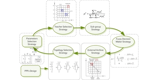
A flowchart of the proposed multi-objective TLBO is shown in Figure 5. The pseudo-code of the proposed method is shown in the following steps:
- Step 1: Initialize population;
- Step 2: Determine the type of group and score criteria for each sub-group;
- Step 3: Evaluate the multi-objective functions with multi-constraints;
- Step 4: Store the first NDS in the external archive.
Figure 5.
Flowchart of the proposed multi-objective TLBO method.

While iter ≤ maximum number of iterations,
- Step 5: Select the teacher for each sub-group using roulette wheel selection;
- Step 6: Divide learners into sub-groups randomly;
- Step 7: Update the grades of learners if the evaluation criteria for each sub-group are satisfied;
- Step 8: Evaluate the multi-objective functions with multi-constraints;
- Step 9: Store new NDSs in the external archive.
End while loop.
5. Simulation Results
In this study, all computer programs were developed using MATLAB 2016a on a Windows 10-based Intel Core i7-2600 personal computer. A one-line diagram of two ST PPFs is shown in Figure 6. The rated voltage and frequency in this sample system are 11.4 kV and 60 Hz, respectively. The fundamental real power demand was 14,590 kW with a power factor of 0.892 lagging. The short-circuit currents varied from 8268 to 19,695 A. In this study, harmonic loads were regarded as harmonic sources. The fundamental equivalent system impedance, which was assumed to be purely inductive, varied from 0.3342 to 0.7961 Ω. The parameters of the test system are presented in Table 3. The distributions of the harmonic current and voltage without the PPFs are listed in Table 4. The limitations of harmonic voltages and currents are based on the IEEE standard 519-1992 [50]. In Table 4, the fifth harmonic current and the total harmonic distortion of the current violate IEEE standard 519.
5.1. Basic Comparison Study
To confirm the efficiency of the proposed method, a solution obtained by the proposed method was selected and compared with that obtained by the SA proposed in [20]. Furthermore, popular optimization algorithms such as BA, PSO, and GA were used as benchmarks for comparisons. The parameters of the proposed TLBO algorithm are tabulated in Table 5. Table 6 lists the parameters of the other optimization algorithms. A candidate solution with a 0.95 lagging power factor obtained by the proposed method is selected by (29) during the iteration process.
In [20], two sets of ST PPFs with and were used to suppress the harmonic distortion. Table 7 shows the filter parameters obtained by the proposed TLBO, BA, PSO, GA, and SA methods at 0.95 lagging power factor, where inductance is depicted in and capacitance in . The individual harmonic distortions for the current and voltage before and after PPF compensation are shown in Figure 7. From Table 7 and Figure 7, the performance of the PPF parameters obtained by the proposed TLBO-based method is better than that of the parameters obtained by other methods. The harmonic distortion of the design solution obtained by the proposed TLBO-based method is listed in Table 8. The performance of the designed filters can be evaluated using a harmonic attenuation factor, as shown in (30). The smaller the harmonic attenuation factor is, the higher is the harmonic current absorbed. The harmonic attenuation factor of the candidate solution is shown in Figure 8. No resonance points were observed. The harmonic currents at critical orders can be significantly reduced by the candidate solution.
where
- harmonic currents through power supply terminal;
- harmonic currents;
- system impedance;
- filter impedance.
Figure 7.
Individual harmonic distortions before and after compensation (a) current and (b) voltage.
Figure 7.
Individual harmonic distortions before and after compensation (a) current and (b) voltage.

Figure 8.
Harmonic attenuation factor with respect to harmonic order of the candidate solution.


Table 7.
Comparisons of PPFs design results with various methods (PF = 0.95).
| Method | TLBO | BA | PSO | GA | SA |
|---|---|---|---|---|---|
| Single-tuned () | |||||
| Single-tuned () | |||||
| (%) | 4.65 | 4.82 | 4.84 | 4.87 | 4.80 |
| (%) | 3.05 | 3.11 | 3.12 | 3.12 | 3.11 |
| Cost | 545.46 | 546.55 | 547.23 | 572.47 | 545.99 |
Table 8.
Harmonic distortion of the design solution obtained by the proposed TLBO-based method.
| Harmonic Orders | Current, A | Voltage, V | Current, % | Voltage, % | IEEE Standard 519 | |
|---|---|---|---|---|---|---|
| Current, % | Voltage, % | |||||
| 2 | 7.26 | 11.55 | 0.93 | 0.18 | 1 | 3 |
| 3 | 9.85 | 23.51 | 1.27 | 0.36 | 4 | 3 |
| 4 | 4.54 | 14.45 | 0.58 | 0.22 | 1 | 3 |
| 5 | 25.13 | 100.03 | 3.23 | 1.52 | 4 | 3 |
| 7 | 15.91 | 88.64 | 2.04 | 1.35 | 4 | 3 |
| 11 | 13.53 | 118.51 | 1.74 | 1.80 | 2 | 3 |
| 13 | 8.31 | 86.03 | 1.07 | 1.31 | 2 | 3 |
| THD (%) | 4.65 | 3.05 | - | - | 5 | 5 |
5.2. Accuracy Study
The proposed algorithm was executed 20 times with 500 iterations to check the distribution of the Pareto front solutions. The final solutions obtained by the proposed TLBO-based method are shown in Figure 9. The Pareto front solutions obtained by Monte Carlo simulations are shown in Figure 10. The generational distance (GD) was used to determine the accuracy of the proposed method [51] as follows:
where is the Euclidean distance between the solution and nearest member in the true Pareto solution set, and is the number of final solutions. The smaller the GD, the closer it is to the true Pareto solution set.
In [40,41], the GDs of MOBA and MOPSO were compared. The GD obtained by the MOBA was better. The behaviors of MOBA and MOPSO were similar. Both are population-based optimization algorithms without a replacement strategy between the previous and current generations. The distribution of the Pareto front solutions formed by these types of optimization algorithms is broad. Therefore, MOBA and MOPSO were used as benchmarks for comparison. As shown in Table 9, the GD results obtained by the proposed MOTLBO were better than those obtained by MOBA and MOPSO.
5.3. Performance Test
To achieve a complete PPF design, the selection mechanisms of topology combinations and parameters for PPFs are imperative. Generally, it is assumed that topology combinations of PPFs are known. In practice, this is not a realistic situation. Therefore, a selection strategy for the topology combination of PPFs was used in this study. The procedure of the selection strategy to determine the topology combination of the PPFs is as follows:
- Step 1: Check individual harmonic distortion; the individual harmonic distortion is evaluated for the node candidates.
- Step 2: Select the maximum number of PPF combinations; the harmonic limit violations set the maximum number of PPFs.
- Step 3: Select the pivot point; to develop a harmonic suppression strategy, a pivot point needs to be selected for the harmonic components. The pivot point is determined by the distribution of the major harmonic components. In most cases, the fifth-order harmonic is regarded as the pivot point.
- Step 4: Determine the possible combinations of PPFs; once the pivot point is determined, the corresponding topology combination of PPFs can be selected to eliminate the major harmonic components. The following rules can determine the topology combination of PPFs: (1) If the major harmonic component occurs at the pivot point, all types of PPFs can be regarded as candidates for evaluation; (2) if the major harmonic components occur below the pivot point (i.e., second-, third-, and fourth-order harmonics), the ST and CD PPFs are regarded as candidates for evaluation; (3) conversely, if the major harmonic components occur above the pivot point (i.e., seventh-, ninth-, eleventh-, and high-order harmonics), the SD and TD PPFs are regarded as candidates for evaluation.
- Step 5: Verify the feasible combinations of PPFs; the initial number and possible combination of PPFs are selected in accordance with the above rules. Not all combinations of PPFs can be used to search for the NDSs for PPF design. If the first NDS for PPF design can be found in a limited number of the initial population, this topology combination of PPFs can be regarded as a feasible combination of PPFs. Otherwise, proceed to Step 6.
- Step6: Recheck individual harmonic distortions; the individual harmonic distortion with the existing PPFs is reevaluated to determine the additional combinations of PPFs.
- Step 7: Determine the additional combinations of PPFs; according to the remaining major harmonic components, the additional combinations of PPFs are generated by the above rules. The feasible combinations of PPFs are verified until the number of PPFs exceeds the predefined threshold.
In this case, the fifth harmonic current and THDI exceeded the tolerance limit. Therefore, the possible combinations of PPFs are ST, SD, TD, CD, ST-ST, ST-SD, ST-TD, ST-CD, SD-SD, SD-TD, TD-TD, and CD-CD. However, the feasible combinations of PPFs were ST, ST-ST, ST-SD, and ST-TD. The first NDS for PPF design can be found in these topology combinations of PPFs within the maximum initial IC. The Pareto solutions with minimum and maximum cost under various types of PPF combinations are listed in Table 10. The THDI did not significantly improve with a single ST PPF. However, an ST PPF can be used to improve the reactive power. The double-ST PPFs with the minimum cost can significantly improve the THDI and THDV. Combining an ST and an SD PPF with the maximum cost can considerably suppress the THDV. Although an ST and a TD PPF can mitigate the THDI and THDV within the harmonic limits, the cost is higher than the other combinations. In terms of cost considerations, the double-ST PPF combination is ranked first. In terms of THDV suppression, the ST and SD PPF combinations were ranked first.
6. Conclusions
In this study, a multi-objective TLBO algorithm for optimizing parameters for PPF design was successfully proposed. Four objective functions were considered in this study: (1) total harmonic distortion of current, (2) total distortion of voltage, (3) IC, and (4) total fundamental reactive power compensation. With the external archive, the NDSs were stored to deal with multi-objective problems for the optimal design of the PPF set. To improve the diversity of NDSs, the sub-group search strategy and teacher selection strategy were used. In addition, a selection mechanism for topology combinations for PPFs was proposed. This study used a sample system with two sets of ST PPFs as a benchmark system for comparison. With the same characteristic harmonic order and reactive power compensation, the harmonic currents at critical orders can be significantly reduced using the candidate solution. In terms of THDI, THDV, and cost, the performance of the proposed TLBO method was better than those of the BA, PSO, GA, and SA methods for basic comparison studies. In terms of the GDs, the proposed TLBO method was better than the MOBA and MOPSO methods for accuracy studies. With the proposed selection mechanisms for the topology combinations and parameters for PPFs, the best compromise solution for a complete PPF design was achieved. In terms of cost considerations, the double-ST PPF combination was ranked first. In terms of THDV suppression, the ST and SD PPF combinations were ranked first. The results show that the proposed method exhibits good performance for improving power supply reliability and ensuring power quality while controlling costs.
Author Contributions
Conceptualization, N.-C.Y.; Data curation, N.-C.Y.; Funding acquisition, N.-C.Y.; Investigation, N.-C.Y. and S.-W.L.; Methodology, N.-C.Y. and S.-W.L.; Resources, N.-C.Y.; Software, N.-C.Y. and S.-W.L.; Supervision, N.-C.Y.; Validation, N.-C.Y. and S.-W.L.; Writing—original draft, N.-C.Y.; Writing—review & editing, N.-C.Y. Both authors have read and agreed to the published version of the manuscript.
Funding
This work was partially supported by the Ministry of Science and Technology (MOST) in Taiwan (MOST 109-3111-8-011-001) and Delta–NTUST Joint Research Center.
Institutional Review Board Statement
Not applicable.
Informed Consent Statement
Not applicable.
Data Availability Statement
Not applicable.
Acknowledgments
This work was partially supported by the Ministry of Science and Technology of Taiwan. The authors would like to thank the funding provided by MOST (MOST 109-3111-8-011-001) and DELTA-NTUST Joint Research Center.
Conflicts of Interest
The authors declare no conflict of interest.
Nomenclature
| the capacitance of j-th filter of type i; | |
| , | upper and lower limits of percentage variation of capacitance for a PPF; |
| Euclidean distance; | |
| rms of fundamental current; | |
| rms of harmonic current with integer order; | |
| harmonic currents; | |
| harmonic currents through power supply terminal; | |
| vector of an objective function; | |
| , | upper and lower limits of percentage variation of frequency for a power system; |
| , | upper and lower bounds of the i-th objective function; |
| inequality constraint; | |
| GD | generational distance; |
| highest harmonic order considered; | |
| upper tolerance for harmonic current at h-th order; | |
| upper tolerance for harmonic voltage at h-th order; | |
| harmonic order; | |
| order of critical harmonic; | |
| order of harmonic to be mitigated; | |
| equality constraint; | |
| to | cost weighting coefficients; |
| , | upper and lower limits of the percentage variation of inductance for a PPF; |
| the inductance of j-th filter of type i; | |
| number of non-dominated solutions in the external archive; | |
| mean grade of the learners in subject j at the i-th iteration; | |
| number of filters of type i; | |
| number of objective functions; | |
| number of inequality constraints; | |
| number of equality constraints; | |
| power loss of j-th filter of type i; | |
| reactive power capacity of j-th filter of type i; | |
| total fundamental reactive power; | |
| fundamental reactive power produced by j-th filter of i-th type; | |
| , | upper and lower limits of reactive power compensation; |
| , | upper and lower limit of percentage variation of resistance for a PPF; |
| resistance of j-th filter of type i; | |
| random number in the range [0,1]; | |
| teaching factor; | |
| upper tolerance for total harmonic distortions of currents; | |
| upper tolerance for total harmonic distortions of voltages; | |
| rms of fundamental voltage; | |
| rms of harmonic voltage with integer order; | |
| grade of the teacher in the subject j at the i-th iteration; | |
| grade of learner k in subject j at the i-th iteration; | |
| vector of decision variables; | |
| the impedance of j-th filter of i-th type; | |
| the impedance of multiple passive power filters; | |
| filter impedance; | |
| system impedance; | |
| set coefficient for i-type filter; | |
| harmonic attenuation factor; | |
| the weighting factor of objective function I; | |
| membership value of the i-th objective function ; | |
| nominal membership value for the non-dominated solution k. |
References
- Eroğlu, H.; Cuce, E.; Cuce, P.M.; Gul, F.; Iskenderoğlu, A. Harmonic problems in renewable and sustainable energy systems: A comprehensive review. Sustain. Energy Technol. Assess. 2021, 48, 101566. [Google Scholar] [CrossRef]
- Baliyan, A.; Jamil, M.; Rizwan, M. Power Quality Improvement Using Harmonic Passive Filter in Distribution System. In Advances in Energy Technology; Springer: Berlin/Heidelberg, Germany, 2021; pp. 435–445. [Google Scholar] [CrossRef]
- Gheisarnejad, M.; Mohammadi-Moghadam, H.; Boudjadar, J.; Khooban, M.H. Active Power Sharing and Frequency Recovery Control in an Islanded Microgrid with Nonlinear Load and Nondispatchable DG. IEEE Syst. J. 2019, 14, 1058–1068. [Google Scholar] [CrossRef]
- Ismael, S.M.; Aleem, S.H.A.; Abdelaziz, A.Y.; Zobaa, A.F. State-of-the-art of hosting capacity in modern power systems with distributed generation. Renew. Energy 2018, 130, 1002–1020. [Google Scholar] [CrossRef]
- Li, D.; Yang, K.; Zhu, Z.Q.; Qin, Y. A Novel Series Power Quality Controller with Reduced Passive Power Filter. IEEE Trans. Ind. Electron. 2016, 64, 773–784. [Google Scholar] [CrossRef]
- Mboving, A.; Stéphane, C. Investigation on the Work Efficiency of the LC Passive Harmonic Filter Chosen Topologies. Electronics 2021, 10, 896. [Google Scholar] [CrossRef]
- Bollen, M.H.J.; Das, R.; Djokic, S.; Ciufo, P.; Meyer, J.; Rönnberg, S.; Zavodam, F. Power Quality Concerns in Implementing Smart Distribution-Grid Applications. IEEE Trans. Smart Grid 2016, 8, 391–399. [Google Scholar] [CrossRef] [Green Version]
- Kalair, A.; Abas, N.; Kalair, A.; Saleem, Z.; Khan, N. Review of harmonic analysis, modeling and mitigation techniques. Renew. Sustain. Energy Rev. 2017, 78, 1152–1187. [Google Scholar] [CrossRef]
- Gandoman, F.H.; Ahmadi, A.; Sharaf, A.M.; Siano, P.; Pou, J.; Hredzak, B.; Agelidis, V.G. Review of FACTS technologies and applications for power quality in smart grids with renewable energy systems. Renew. Sustain. Energy Rev. 2018, 82, 502–514. [Google Scholar] [CrossRef]
- Yang, N.; Le, M. Three-phase harmonic power flow by direct Z BUS method for unbalanced radial distribution systems with passive power filters. IET Gener. Transm. Distrib. 2016, 10, 3211–3219. [Google Scholar] [CrossRef]
- Yang, N.-C.; Le, M.-D. Loop frame of reference based harmonic power flow for unbalanced radial distribution systems. Int. J. Electr. Power Energy Syst. 2016, 77, 128–135. [Google Scholar] [CrossRef]
- Yang, N. Three-phase power flow calculations using direct Z BUS method for large-scale unbalanced distribution networks. IET Gener. Transm. Distrib. 2016, 10, 1048–1055. [Google Scholar] [CrossRef]
- Yang, N.-C.; Tseng, W.-C. Adaptive three-phase power-flow solutions for smart grids with plug-in hybrid electric vehicles. Int. J. Electr. Power Energy Syst. 2015, 64, 1166–1175. [Google Scholar] [CrossRef]
- Yang, N. Three-phase power flow calculations by direct Z LOOP method for microgrids with electric vehicle charging demands. IET Gener. Transm. Distrib. 2013, 7, 1002–1010. [Google Scholar] [CrossRef]
- Chen, T.-H.; Yang, N.-C. Simplified annual energy loss evaluation method for branch circuits of a home or building. Energy Build. 2010, 42, 2281–2288. [Google Scholar] [CrossRef]
- Yang, N.-C.; Chen, T.-H. Assessment of loss factor approach to energy loss evaluation for branch circuits or feeders of a dwelling unit or building. Energy Build. 2012, 48, 91–96. [Google Scholar] [CrossRef]
- Yang, N.-C.; Tseng, W.-C. Impact assessment of a hybrid energy-generation system on a residential distribution system in Taiwan. Energy Build. 2015, 91, 170–179. [Google Scholar] [CrossRef]
- Yang, N.-C.; Chen, H.-C. Decomposed Newton algorithm-based three-phase power-flow for unbalanced radial distribution networks with distributed energy resources and electric vehicle demands. Int. J. Electr. Power Energy Syst. 2018, 96, 473–483. [Google Scholar] [CrossRef]
- Yang, N.; Chen, H. Three-phase power-flow solutions using decomposed quasi-Newton method for unbalanced radial distribution networks. IET Gener. Transm. Distrib. 2017, 11, 3594–3600. [Google Scholar] [CrossRef]
- Chou, C.-J.; Liu, C.-W.; Lee, J.-Y.; Lee, K.-D. Optimal planning of large passive-harmonic-filters set at high voltage level. IEEE Trans. Power Syst. 2000, 15, 433–441. [Google Scholar] [CrossRef] [Green Version]
- Chen, Y.-M. Passive filter design using genetic algorithms. IEEE Trans. Ind. Electron. 2003, 50, 202–207. [Google Scholar] [CrossRef]
- Makram, E.; Subramaniam, E.; Girgis, A.; Catoe, R. Harmonic filter design using actual recorded data. IEEE Trans. Ind. Appl. 1993, 29, 1176–1183. [Google Scholar] [CrossRef]
- Das, J. Passive Filters—Potentialities and Limitations. IEEE Trans. Ind. Appl. 2004, 40, 232–241. [Google Scholar] [CrossRef]
- Chang, G.W.; Wang, H.-L.; Chuang, G.-S.; Chu, S.-Y. Passive Harmonic Filter Planning in a Power System with Considering Probabilistic Constraints. IEEE Trans. Power Deliv. 2008, 24, 208–218. [Google Scholar] [CrossRef]
- He, N.; Xu, D.; Huang, L. The Application of Particle Swarm Optimization to Passive and Hybrid Active Power Filter Design. IEEE Trans. Ind. Electron. 2009, 56, 2841–2851. [Google Scholar] [CrossRef]
- Chang, Y.-P.; Tseng, W.-K.; Tsao, T.-F. Application of combined feasible-direction method and genetic algorithm to optimal planning of harmonic filters considering uncertainty conditions. IEE Proc.-Gener. Transm. Distrib. 2005, 152, 729–736. [Google Scholar] [CrossRef]
- Ko, C.-N.; Chang, Y.-P.; Wu, C.-J. A PSO Method with Nonlinear Time-Varying Evolution for Optimal Design of Harmonic Filters. IEEE Trans. Power Syst. 2008, 24, 437–444. [Google Scholar] [CrossRef]
- Chu, R.; Wang, J.-C.; Chiang, H.-D. Strategic planning of LC compensators in nonsinusoidal distribution systems. IEEE Trans. Power Deliv. 1994, 9, 1558–1563. [Google Scholar] [CrossRef]
- Ortmeyer, T.; Hiyama, T. Distribution system harmonic filter planning. IEEE Trans. Power Deliv. 1996, 11, 2005–2012. [Google Scholar] [CrossRef]
- Chang, G.W.; Wang, H.-L.; Chu, S.-Y. Strategic placement and sizing of passive filters in a power system for controlling voltage distortion. IEEE Trans. Power Deliv. 2004, 19, 1204–1211. [Google Scholar] [CrossRef]
- Nassif, A.B.; Xu, W.; Freitas, W. An Investigation on the Selection of Filter Topologies for Passive Filter Applications. IEEE Trans. Power Deliv. 2009, 24, 1710–1718. [Google Scholar] [CrossRef]
- Kawann, C.; Emanuel, A. Passive shunt harmonic filters for low and medium voltage: A cost comparison study. IEEE Trans. Power Syst. 1996, 11, 1825–1831. [Google Scholar] [CrossRef]
- Lin, K.-P.; Lin, M.-H.; Lin, T.-P. An advanced computer code for single-tuned harmonic filter design. IEEE Trans. Ind. Appl. 1998, 34, 640–648. [Google Scholar] [CrossRef]
- Bajaj, M.; Sharma, N.K.; Pushkarna, M.; Malik, H.; Alotaibi, M.A.; Almutairi, A. Optimal Design of Passive Power Filter Using Multi-Objective Pareto-Based Firefly Algorithm and Analysis Under Background and Load-Side’s Nonlinearity. IEEE Access 2021, 9, 22724–22744. [Google Scholar] [CrossRef]
- Badugu, R.; Acharya, D.; Das, D.K.; Prakash, M. Class Topper Optimization Algorithm based Optimum Passive Power Filter Design for Power System. In Proceedings of the 2021 5th International Conference on Computing Methodologies and Communication (ICCMC), Erode, India, 8–10 April 2021; pp. 648–652. [Google Scholar]
- Wang, Y.; Liu, H.; Yin, K.; Yuan, Y. A Full-Tuned Filtering Method for Dynamic Tuning Passive Filter Power Electronics. J. Control. Autom. Electr. Syst. 2021, 1–11. [Google Scholar] [CrossRef]
- Wang, Y.; Yin, K.; Liu, H.; Yuan, Y. A Method for Designing and Optimizing the Electrical Parameters of Dynamic Tuning Passive Filter. Symmetry 2021, 13, 1115. [Google Scholar] [CrossRef]
- Azab, M. Multi-objective design approach of passive filters for single-phase distributed energy grid integration systems using particle swarm optimization. Energy Rep. 2019, 6, 157–172. [Google Scholar] [CrossRef]
- Wang, S.; Ding, X.; Wang, J. Multi-objective optimization design of passive filter based on particle swarm optimization. In Proceedings of the Journal of Physics: Conference Series. J. Physics Conf. Ser. 2020, 1549, 032017. [Google Scholar] [CrossRef]
- Yang, N.; Le, M. Multi-objective bat algorithm with time-varying inertia weights for optimal design of passive power filters set. IET Gener. Transm. Distrib. 2015, 9, 644–654. [Google Scholar] [CrossRef]
- Yang, N.-C.; Le, M.-D. Optimal design of passive power filters based on multi-objective bat algorithm and pareto front. Appl. Soft Comput. 2015, 35, 257–266. [Google Scholar] [CrossRef]
- Rao, R.; Savsani, V.; Vakharia, D. Teaching–learning-based optimization: A novel method for constrained mechanical design optimization problems. Comput. Des. 2011, 43, 303–315. [Google Scholar] [CrossRef]
- Rao, R.V.; Kalyankar, V. Parameter optimization of modern machining processes using teaching–learning-based optimization algorithm. Eng. Appl. Artif. Intell. 2013, 26, 524–531. [Google Scholar] [CrossRef]
- Nayak, M.; Nayak, C.; Rout, P. Application of Multi-Objective Teaching Learning based Optimization Algorithm to Optimal Power Flow Problem. Procedia Technol. 2012, 6, 255–264. [Google Scholar] [CrossRef] [Green Version]
- Niknam, T.; Azizipanah-Abarghooee, R.; Narimani, M.R. A new multi objective optimization approach based on TLBO for location of automatic voltage regulators in distribution systems. Eng. Appl. Artif. Intell. 2012, 25, 1577–1588. [Google Scholar] [CrossRef]
- Lata, P.; Vadhera, S. Reliability Improvement of Radial Distribution System by Optimal Placement and Sizing of Energy Storage System using TLBO. J. Energy Storage 2020, 30, 101492. [Google Scholar] [CrossRef]
- Lata, P.; Vadhera, S. TLBO-based approach to optimally place and sizing of energy storage system for reliability enhancement of radial distribution system. Int. Trans. Electr. Energy Syst. 2020, 30, e12334. [Google Scholar] [CrossRef]
- Coello, C.C.; Toscano-Pulido, G.; Lechuga, M. Handling multiple objectives with particle swarm optimization. IEEE Trans. Evol. Comput. 2004, 8, 256–279. [Google Scholar] [CrossRef]
- Shabanpour-Haghighi, A.; Seifi, A.R.; Niknam, T. A modified teaching–learning based optimization for multi-objective optimal power flow problem. Energy Convers. Manag. 2014, 77, 597–607. [Google Scholar] [CrossRef]
- IEEE Std 519-1992. Recommended Practices and Requirements for Harmonic Control in Electrical Power System; IEEE Industry Applications Society: New York, NY, USA, 1993. [Google Scholar]
- Van Veldhuizen, D.A.; Lamont, G.B. Multiobjective Evolutionary Algorithm Research: A History and Analysis, 1998. Citeseer. Available online: http://citeseerx.ist.psu.edu/viewdoc/summary?doi=10.1.1.35.8924 (accessed on 18 August 2021).
Figure 1.
Typical PPFs: (a) ST PPF, (b) SD PPF, (c) TD PPF, and (d) CD PPF.

Figure 2.
NDSs in a two-objective problem.

Figure 3.
Insertion of an NDS when the external archive is full.

Figure 6.
One-line diagram with two single-tuned filters.

Figure 9.
Pareto front set obtained by the proposed TLBO-based method: (a) voltage THD vs. current THD; (b) current THD vs. cost; (c) voltage THD vs. cost; (d) reactive power compensation vs. cost.
Figure 9.
Pareto front set obtained by the proposed TLBO-based method: (a) voltage THD vs. current THD; (b) current THD vs. cost; (c) voltage THD vs. cost; (d) reactive power compensation vs. cost.

Figure 10.
Pareto front set obtained by Monte Carlo simulations: (a) voltage THD vs. current THD; (b) current THD vs. cost, (c) voltage THD vs. cost, (d) reactive power compensation vs. cost.
Figure 10.
Pareto front set obtained by Monte Carlo simulations: (a) voltage THD vs. current THD; (b) current THD vs. cost, (c) voltage THD vs. cost, (d) reactive power compensation vs. cost.


Table 1.
The harmonic impedance of PPFs.
| Type | ||
|---|---|---|
| ST | ||
| SD | ||
| TD | ||
| CD |
Table 2.
Set coefficient .
| Set No. | ST | SD | TD | CD |
|---|---|---|---|---|
| 1 | 1 | 1 | 1.2 | 1.2 |
| 2 | 1.2 | 1.4 | 1.6 | 1.6 |
| 3 | 1.6 | 1.8 | 2.0 | 2.0 |
| 4 | 2.0 | 2.2 | 2.4 | 2.4 |
| 5 | 2.4 | 2.5 | 2.8 | 2.8 |
Table 3.
Parameters of the test system.
| Item | Feasible Ranges of Parameters |
|---|---|
| Short-circuit current | 8268–19,695 A |
| System short circuit capacity | 163–388 MVA |
| Equivalent system impedance | 0.3342–0.7961 Ω |
| System voltage level | 11.4 kV |
| System frequency | 60 Hz |
Table 4.
Distributions of harmonic current and voltage without PPFs.
| Harmonic Orders | Current, A | Voltage, V | IEEE Standard 519 | |||
|---|---|---|---|---|---|---|
| Current, A | Current, % | Voltage, V | Voltage, % | |||
| 1 | 828.37 | 6581.79 | - | - | - | - |
| 2 | 7.02 | 11.18 | 8.28 | 1 | 197.5 | 3 |
| 3 | 8.64 | 20.63 | 33.1 | 4 | 197.5 | 3 |
| 4 | 5.92 | 18.85 | 8.28 | 1 | 197.5 | 3 |
| 5 | 45.8 | 182.3 | 33.1 | 4 | 197.5 | 3 |
| 7 | 19.0 | 105.9 | 33.1 | 4 | 197.5 | 3 |
| 11 | 15.4 | 134.9 | 16.6 | 2 | 197.5 | 3 |
| 13 | 9.4 | 97.28 | 16.6 | 2 | 197.5 | 3 |
| THD (%) | 6.55 | 4.11 | - | 5 | - | 5 |
Table 5.
Parameters of the proposed TLBO algorithm.
| Item | Feasible Ranges of Parameters |
|---|---|
| Number of iterations | 200 |
| Population size | 20 |
| Number of objectives | 4 |
| Number of constraints | 22 |
| Number of groups | 4 |
| Size of external archive | 100 |
| Number of divisions | 30 |
| Maximum number of PPFs set | 2 |
| Maximum initial IC | 1000 pu |
| R for PPFs | 0.01–100 Ω |
| L for PPFs | 0.01–50 mH |
| C for PPFs | 0.01–100 μF |
Table 6.
Parameters of the other optimization algorithms.
| Parameter | TLBO | BA | PSO | GA |
|---|---|---|---|---|
| Number of iterations | 200 | 200 | 200 | 200 |
| Population size | 20 | 20 | 20 | 20 |
| Other related parameters | - | Maximum frequency, Minimum frequency, Constants, | Cognitive parameter, Social parameter, | EliteCount = 2; CrossoverFraction = 0.8; MutationRate = 0.1; MaximumSurvivalRate = 2; |
Table 9.
Generational distance—MOTLBO with MOBA and MOPSO.
| Algorithm | Generational Distance | ||||
|---|---|---|---|---|---|
| Best | Worst | Average | Median | Std. Dev. | |
| MOTLBO | 0.00000053 | 0.0013 | 0.0000689 | 0.0000571 | 0.000068 |
| MOBA | 0.00000094 | 0.0106 | 0.0000921 | 0.0000708 | 0.000220 |
| MOPSO | 0.00000193 | 0.0177 | 0.0001251 | 0.0000874 | 0.000566 |
Table 10.
Pareto solutions with minimum cost and maximum cost.
| Type of Filters | Parameter | THDI | THDV | PF | QF | Cost | |||||
| * | |||||||||||
| ST | 4.60 | 86.35 | 4.99 | 2.98 | 0.98 | 4484 | 635 | ||||
| ST | 4.07 | 96.35 | 4.83 | 2.88 | 0.99 | 4999 | 705 | ||||
| ST | 11.05 | 26.58 | 3.77 | 2.74 | 0.95 | 2596 | 538 | ||||
| ST | 18.31 | 23.69 | |||||||||
| ST | 10.31 | 28.47 | 3.73 | 2.68 | 0.96 | 3024 | 592 | ||||
| ST | 14.22 | 30.07 | |||||||||
| ST | 10.16 | 28.89 | 4.01 | 2.80 | 0.96 | 3064 | 589 | ||||
| SD | 20.96 | 8.68 | 31.18 | ||||||||
| ST | 9.81 | 29.95 | 3.87 | 2.53 | 0.99 | 5609 | 929 | ||||
| SD | 20.54 | 5.67 | 78.06 | ||||||||
| ST | 10.16 | 29.19 | 4.10 | 2.92 | 0.95 | 2606 | 788 | ||||
| TD | 38.41 | 23.45 | 21.01 | 21.01 | |||||||
| ST | 9.07 | 33.04 | 4.20 | 2.85 | 0.98 | 4652 | 1254 | ||||
| TD | 47.81 | 31.83 | 46.27 | 46.27 | |||||||
* ST: single-tuned, SD: second-order damped, TD: third-order damped, and CD: C-type damped.
Publisher’s Note: MDPI stays neutral with regard to jurisdictional claims in published maps and institutional affiliations. |
© 2021 by the authors. Licensee MDPI, Basel, Switzerland. This article is an open access article distributed under the terms and conditions of the Creative Commons Attribution (CC BY) license (https://creativecommons.org/licenses/by/4.0/).
Share and Cite
MDPI and ACS Style
Yang, N.-C.; Liu, S.-W. Multi-Objective Teaching–Learning-Based Optimization with Pareto Front for Optimal Design of Passive Power Filters. Energies 2021, 14, 6408. https://0-doi-org.brum.beds.ac.uk/10.3390/en14196408
AMA Style
Yang N-C, Liu S-W. Multi-Objective Teaching–Learning-Based Optimization with Pareto Front for Optimal Design of Passive Power Filters. Energies. 2021; 14(19):6408. https://0-doi-org.brum.beds.ac.uk/10.3390/en14196408
Chicago/Turabian StyleYang, Nien-Che, and Sun-Wei Liu. 2021. "Multi-Objective Teaching–Learning-Based Optimization with Pareto Front for Optimal Design of Passive Power Filters" Energies 14, no. 19: 6408. https://0-doi-org.brum.beds.ac.uk/10.3390/en14196408
Note that from the first issue of 2016, this journal uses article numbers instead of page numbers. See further details here.