
Non-Isothermal Vortex Flow in the T-Junction Pipe
by
 and
and
Tatyana A. Baranova
1, 
Yulia V. Zhukova
1,
Andrei D. Chorny
1,2,
Artem Skrypnik
3,4,* and
Igor A. Popov
3,* 1
A.V. Luikov Heat and Mass Transfer Institute of NAS of Belarus, 220072 Minsk, Belarus
2
Moscow Engineering Physics Institute, National Research Nuclear University MEPhI, 115409 Moscow, Russia
3
Department of Heat Engineering and Energy Machinery, Kazan National Research Technical University Named after A.N. Tupolev—KAI (KNRTU-KAI), 420111 Kazan, Russia
4
Institute of Process Engineering and Environmental Technology, Technische Universität Dresden, 01062 Dresden, Germany
*
Authors to whom correspondence should be addressed.
Energies 2021, 14(21), 7002; https://0-doi-org.brum.beds.ac.uk/10.3390/en14217002
Submission received: 30 August 2021
/
Revised: 14 October 2021
/
Accepted: 19 October 2021
/
Published: 26 October 2021
(This article belongs to the Special Issue Numerical Simulation of Convective Heat Transfer)
Abstract
:The numerical simulation approach of heat carrier mixing regimes in the T-junction shows that the RANS approach is beneficial for a qualitative flow analysis to obtain relatively agreed averaged velocity and temperature. Moreover, traditionally, the RANS approach only predicts the averaged temperature distribution. This mathematical model did not consider the temperature fluctuation variations important for the thermal fatigue task. It should also be emphasized that unlike the LES approach, the steady RANS approach cannot express a local flow structure in intense mixing zones. Nevertheless, apparently the adopted RANS approach should be used for assessing the quality of computational meshes, boundary conditions with the purpose to take LES for further numerical simulation.
1. Introduction
Modern power engineering is based on using thermal power plants (TPP) operating on organic fuels (their share in world power engineering is ~70%), nuclear power plants (NPP) (their share in world power engineering is 10% to 16%), and water power plants (WPP) (their share in world power engineering is 16% to 20%). In case of emergency situations, the greatest harm to the environment can be made by TPPs and NPPs. According to statistics, about 90% of major accidents at TPPs are caused by equipment failure and accompanied by fires, and 10% is the result of damage to building constructions. The share of accidents that have occurred in engine rooms is 72%, with 23% in boiler rooms, and about 5% in cable tunnels [1].
One of the requirements of reliable assessment of heat carrier thermal and hydraulic parameters in different elements of thermal power equipment (TPE) (boilers, different-design steam generators, heat exchangers, pipelines, fuel elements, and other heat-loaded elements of nuclear reactor plants, etc.) is that heat loads (first of all, thermal and hydraulic) occurring in such plants can give rise to thermal fatigue and mechanical vibrations under normal TPE conditions [2]. Historically, the hydrodynamic flow and hydraulic shock stability problem (the pipe and pipe junction strength problem) is quite old, for example, see Professor Zhukovsky’s classical work “About hydraulic shock in water pipes” [3]. Thermal and hydraulic assessments are used as the initial data for solution of cyclic strength and brittle failure tasks with the purpose to analyze the stress–strain state and strength of TPE elements [2]. Convective heat transfer processes in such elements as a rule are accompanied by temperature fluctuations. These fluctuations manifest themselves at boiling crises, unstable steam generation on heated surfaces, heat carrier flowrate fluctuations, unsteady convective transfer, etc. Temperature fluctuations cause wall temperature stresses to change significantly. In combination with hydraulic load and corrosion of the heat carrier operating medium, they can destruct TPE elements [2]. This is illustrative of such phenomena as emergency situations: the failure of the structural elements of a nuclear power plant (NPP Sivo (France) 1998; on power unit No. 1, the radioactive water leak from the first heat carrier circuit due to forming pipe cracks; NPP Genkai (Japan), 1998; the leak in the capacitor of power unit No.1, 2011; the leak in the cooling system of power unit No. 3; NPP Tiange (Belgium), 2012; the outer shell erosion of power unit No. 2; NPP Farley (USA), 2013; the unplanned carbon dioxide emission on power unit No. 2; NPP Tsuruga (Japan), 1981; the radiation emission on power unit No. 2, the discharge of 16 tons of radiative water; NPP Loviisa (Finland), 1990; accidents on power unit No. 1, the main pipeline failure and erosion-corrosion failures of pipelines at the junction of flow meters; NPP Novovoronezh (USSR), 1990; on power unit No. 5, the weld failure of the pipe valve due to the corrosion-mechanical welding defects (lack of root penetration) developing when acted upon by operation factors).
The task of predicting thermal fatigue and mechanical vibration impact is quite labor-intensive since it needs to determine both hydrodynamic and temperature parameters in near-wall flows of working media, to calculate thermal conductivity and mechanical stresses in solid materials of the walls of TPE elements, as well as in the most unfavorable cases, for example, to analyze the influence on the strength of forming fractures, etc. [3]. Usually, thermal fatigue and mechanical stress are calculated in two main stages. At the first stage, the task of hydrodynamics and heat transfer in flows of working media is solved with allowance for the geometric features of TPE elements. At the second stage, the stress–strain state of TPE elements is determined, when the obtained temperature fields, as well as hydrodynamic ones are used as a load source. In this situation, calculations or numerical simulation of geometrically simple TPE elements, which qualitatively reproduce a separate physical effect, are important for the understanding of this effect, the validity of the used mathematical model, and the reliability of thermal and hydraulic calculation. For example, as applied to NPP reactor plants, thermal fatigue is studied for two test geometric configurations: (a) T-junction, (b) two or more co-current jets issuing into the wall-bounded space [4]. The T-junction is a widely used component, with the help of which pipelines are combined in different TPE systems.
In the thermal shock analysis, besides two-phase flow problems (ECC injection jet mixing, stratified flow in the cold leg), one-phase mixing problems are also of importance. This is mixing of water streams with different temperature and, therefore, with different densities in the downcomer. The CFD simulation of buoyancy-driven mixing is still a challenge, as advanced turbulence models taking into account the additional shear stress generation by buoyancy forces are necessary. This might be the Reynolds stress models, large eddy or detached eddy simulation. Mixing tees are the inevitable piping structures in fossil fuel and nuclear power plants. When high- and low-temperature flows are mixing in the mixing tee, high-cycle thermal fatigue may occur. Fatigue cracks have been often found downstream behind the mixing tee, for example in the Civaux-1 [5] and more recently in U.S nuclear power plants [6]. Hence thermal fatigue is one of the major degradation mechanisms that must be considered in nuclear and fossil fuel power plant management. Other applications can also illustrate the benefit of using of CFD codes in order to assess specific-type flows in PWR reactors such as temperature fluctuations inducing thermal fatigue. For example, a configuration, related to a mixing zone in a PWR reactor, consists of a T-junction upstream of a bend, in which hot and cold fluids interact, creating temperature fluctuations that might result in thermal fatigue. The use of the thermal coupling between a CFD code with a solid thermal code gives access to an instantaneous temperature field inside the fluid and the solid. In order to capture fluctuations, large eddy simulation may be required for such a problem. CFD is also used in other components of the primary cooling system such as the heat carrier main pump where it can help avoid cavitation erosion in every operating conditions. Other studies concerned with the temperature fluctuations within the thermal barrier of the pump and around the shaft that together with high radial loadings on the impeller can lead to shaft crackings.
To understand the thermal fatigue mechanism, experiments under actual plant conditions are inevitable. The FATHER experiment [7] measured fluid and pipe wall temperatures to observe the temperature fluctuation mechanism in the mixing tee. The fluid-structure-interaction (FSI) test facility [8] was used to measure pipe wall temperature when hot (265 °C) and cold (20 °C) flows were mixed and finally, cracking in the piping material was reproduced. The FATHER experiment and the FSI test facility measurements were carried out under the condition of a high temperature difference (over 150 °C). The Japan Atomic Energy Agency (JAEA) conducted a series of T-junction experiments called the WATLON experiment [9]. The test section was made of transparent acrylic resin, and flow velocity and temperature distributions were measured. Though the WATLON experiment was conducted under a relatively low temperature difference (15 °C), flow velocity and temperature distributions were measured in the whole region of the T-junction to understand the mixing phenomena. Various researchers spent considerable efforts to develop a computational fluid dynamics (CFD) method to simulate the results of the WATLON experiment [9,10,11].
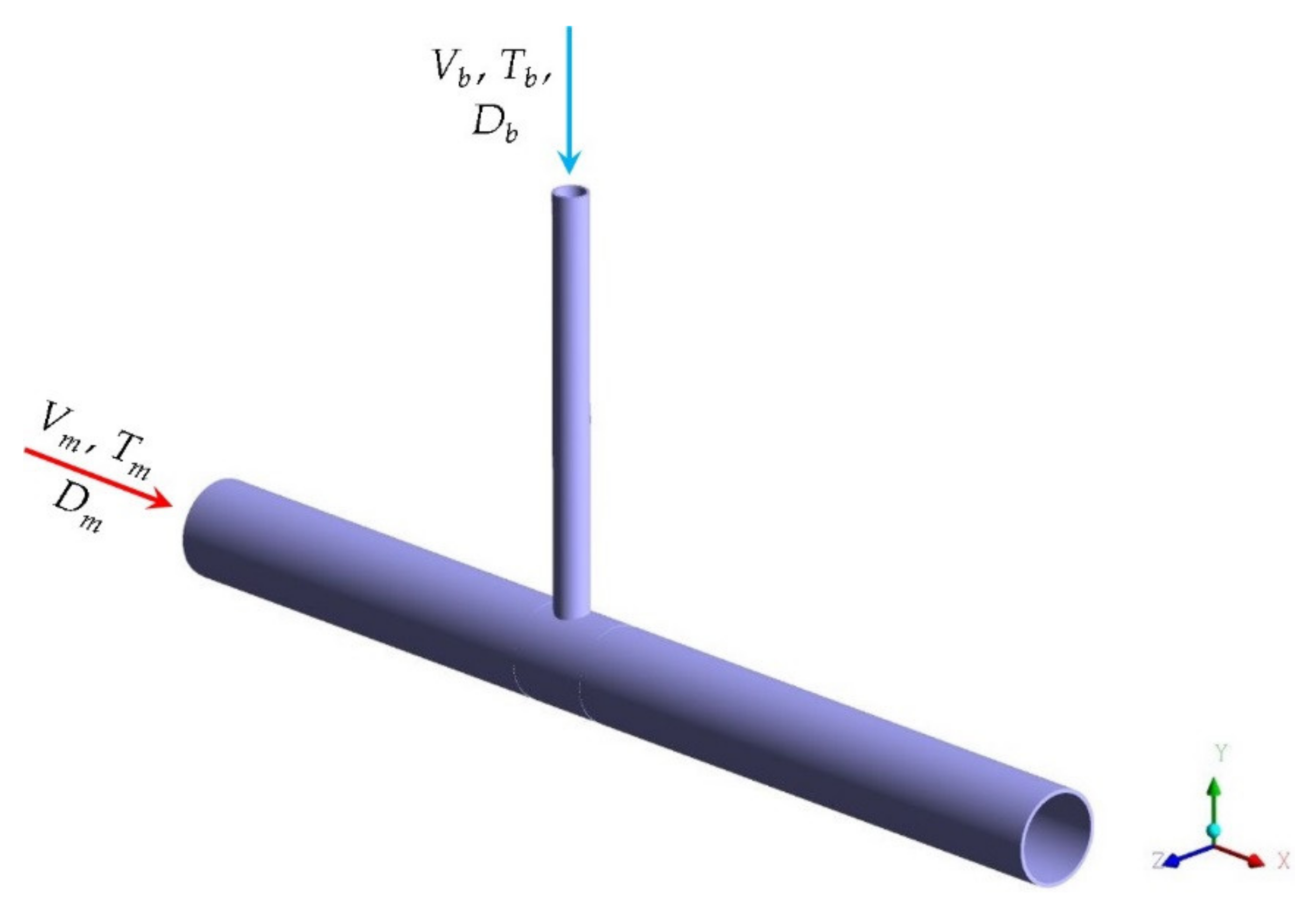
The objective of the present work was to study turbulent mixing of non-isothermal flows in the T-junction using numerical simulation to determine the distribution of hydrodynamic and temperature parameters depending on the mixing regimes in such a junction. Thus, the first-stage task of thermal fatigue prediction in TPE elements was solved. The typical exhaust tee was taken as a variant of the mixing component embodiment of the T-junction. Hot and cold heat carriers were mixed in the exhaust tee (Figure 1). Numerical simulation was performed, assuming that the inner walls of the T-junction were thermally insulated, not considering the heat removal into the walls. It was assumed that in the inlet cross-section of the T-junction, the heat carrier flows had different flowrates and temperatures.
The particular values of the geometric and dynamic parameters corresponded to the WATLON data [9] and the experimental data of the research team of the Stuttgart University, the network research project titled ′Thermal Fatigue—Basics of the system, outflow and material characteristics of piping under thermal fatigue’ [12].
1.1. Mixing Regimes in the T-Junction
These mixing regimes depend on a number of factors. The velocity ratio Vm/Vb or, as proposed in [6], the momentum ratio Mm/Mb is the defining parameter. A significant influence will also be made by the heat carrier temperature ratio Tm/Tb at the inlets of the main pipe and the socket.
Assess the influence of the socket orientation relative to the gravity force action (socket flow direction along or against the gravity force vector). The influence will be significant at natural convection. Since mixing is considered in the water T-junction, the limiting case related to the jet buoyancy within the natural convection regime must be assessed.
At natural convection, the Richardson number, Ri = Gr/Re2 > 1, hence Gr > Re2 or, presenting them in dimensional form, we have , where Re is the Reynolds number and Gr is the Grashof number. Thus,
Work [13] contains the value of the water temperature expansion coefficient β depending on the temperature and pressure. The temperature drop ΔT = 15° is known from the WATLON data [9]. Hence, the location of the socket relative to the gravity force direction affects the nature of water issuing from the socket at the issuing velocity Vb < 0.033 m/s under the considered experiment conditions. Thus, as the experimental data [9,10] show, the socket location is not critical when considering the mixing in the zone where the socket is attached to the main pipe of the T-junction, since Vb ≥ 0.5 m/s for all mixing regimes. The contribution of the mass gravity force is relatively small.
According to [11], the following mixing regimes determined in [9] and cited in Table 1 will be considered. The near-wall jet regime is characterized by the socket jet pressed to the wall of the main pipe where high momentum is available. In the deflecting jet regime, the momentum flows are compared. The socket flow presses the main pipe flow to the upper wall of the channel. The main pipe flow deflects the socket flow from the vertical direction, trying to press it to the lower wall of the channel. In the impact jet regime, the socket flow has a very high velocity in comparison to the main pipe flow one (the socket flow is high). The socket jet blocks the entire cross-section of the main pipe and reaches its upper wall. Thus, bearing in mind the momentum Mm in the main pipe and the momentum Mb in the socket, we can judge about the mixing picture of two flows in the T-junction. We used such an approach for determining the mixing regimes [9,10] (Table 1). The momentum ratio at the inlets of the main pipe and the socket was indicated as Mm/Mb where:
More traditional for flow regimes is the presentation based on the ratio of the Reynolds numbers constructed in terms of the flow parameters at the inlets of the main pipe and the socket. The momentum ratio Mm/Mb and the Reynolds number ratio Rem/Reb are related as follows:
Table 1 cites the mixing regimes vs. the flow Reynolds number ratio in the main pipe and the momentum ratio in the socket.
The experimental study [12] was concerned with two cases of mixing of non-isothermal flows in the T-junction at the fixed mass flowrate ratio Qm/Qb = 1/4. In the first case, the ratio of the Reynolds numbers constructed in terms of the initial parameters was Rem/Reb = 6.6 and the temperature drop ΔT = Tm−Tb = 65° (Table 2, regime ST1). In the second case, Rem/Reb = 12.3 and the temperature drop ΔT = 143° (Table 2, regime ST2). By assessing the initial parameters, a conclusion can be made that the considered heat carrier flow regime in the T-junction is the near-wall jet.
Works [8,12,14] did not assess the influence of the socket location on mixing regimes in the T-junction, although the physical experiments and the LES experiments revealed significant stratification in the main pipe downstream behind the mixing zone. If the assessment used the the above described method, then we can obtain that the issuing velocity from the socket within the regime ST1 must not exceed Vb < 0.168 m/s and within the regime ST2—Vb < 0.25 m/s.
In work [12], for example, it is shown that within the regimes ST1 and ST2, the issuing velocity from the socket is Vb = 0.084 m/s, which evidences that the socket location relative to the direction of mass forces can only affect the processes in the mixing zone of the T-junction, but does not affect the stratification processes in the main pipe downstream
1.2. Numerical Hydrodynamics/Heat Transfer Simulation in the T-Junction
The Reynolds-averaged steady Navier–Stokes equations, the continuity equation, and the energy equation formulated for enthalpy (RANS approach) were solved with the use of numerical simulation. Boussinesq′s eddy viscosity hypothesis and Menter′s shear stress transport κ–ω model [15] were used for closure. The thermophysical properties of heat carrier (density, viscosity, thermal conductivity) were assigned in the form of the temperature-dependent piecewise linear functions.
At the inlets of the main pipe and the socket, the bulk velocity and temperature values were assigned; the turbulence fluctuation level Tu = 1% and the hydraulic diameter were taken as turbulence characteristics to determine the turbulence level at the inlet. The soft boundary conditions in terms of both hydrodynamic and thermal parameters were predetermined at the computational domain outlet. It was assumed that the T-junction walls are thermally insulated. It can be noted that, when the additional task of admixture transport in the T-junction at the wall thermal insulation conditions is solved, the temperature and admixture transport processes will be similar. Conservative scalar theory [16] can be used for analyzing transport processes.
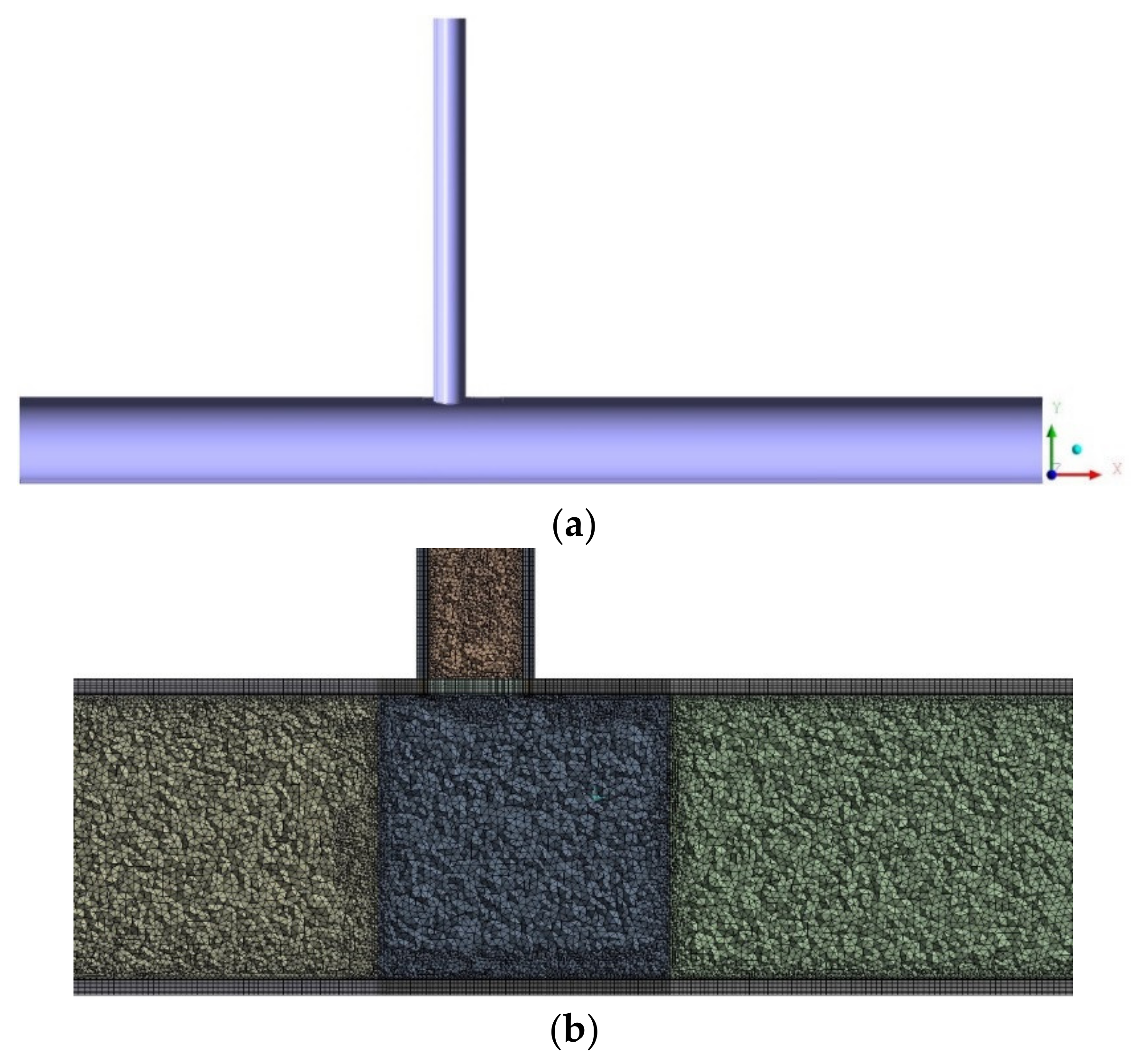
Numerical simulation was performed using the gasdynamic solver Ansys Fluent 19.1. Numerical simulation used the finite volume method [17]. CAD model of the object of investigation presented in Figure 1. Figure 2a shows the cross section of the CAD model. The computational mesh (Figure 2) was condensed in the mixing zone of two flows—the one issuing from the main pipe and the other issuing from the socket. The minimum size of the cell in the near-wall boundary layer was 0.1 mm, the maximum cell size in the flow—4 mm. The cell size was chosen to minimize the influence of artificial viscosity, arising due to the approximation error, on numerical simulation results, i.e., the linear size of the cell provided small artificial viscosity in comparison to effective (molecular + turbulent) viscosity [18]. 3D computational mesh was contained hexahedral and mixed elements. Minimum orthogonal quality was 3.57×10⁻² maximum aspect ratio was 9.03.
Thus, the steady flow of heat carrier was considered. At that, the iteration convergence of searching for a solution meant that the steady flow regime was present. The fact, illustrating the convergence absence when solving such a task, revealed that the unsteady mixing regime was significantly unsteady. The task convergence was controlled through a residual value. Calculations were stopped after achieving a pressure residual value of 10−4 and a temperature residual value of 10−8.
2. Numerical Simulation Results of the Mixing Regimes in the T-Junction
2.1. WATLON Experiment Simulation
Water with a temperature Tm is supplied with a velocity Vm through the main pipe with the inner diameter Dm = 150 mm. At the distance L = 804 mm from the main pipe inlet at an inclination angle of 90°, the socket is placed—the pipe with the inner diameter Db = 50 mm, through which water is supplied at a temperature Tb with a velocity Vb. According to [10,11], for all considered cases, the flow regime corresponded to the turbulent one.
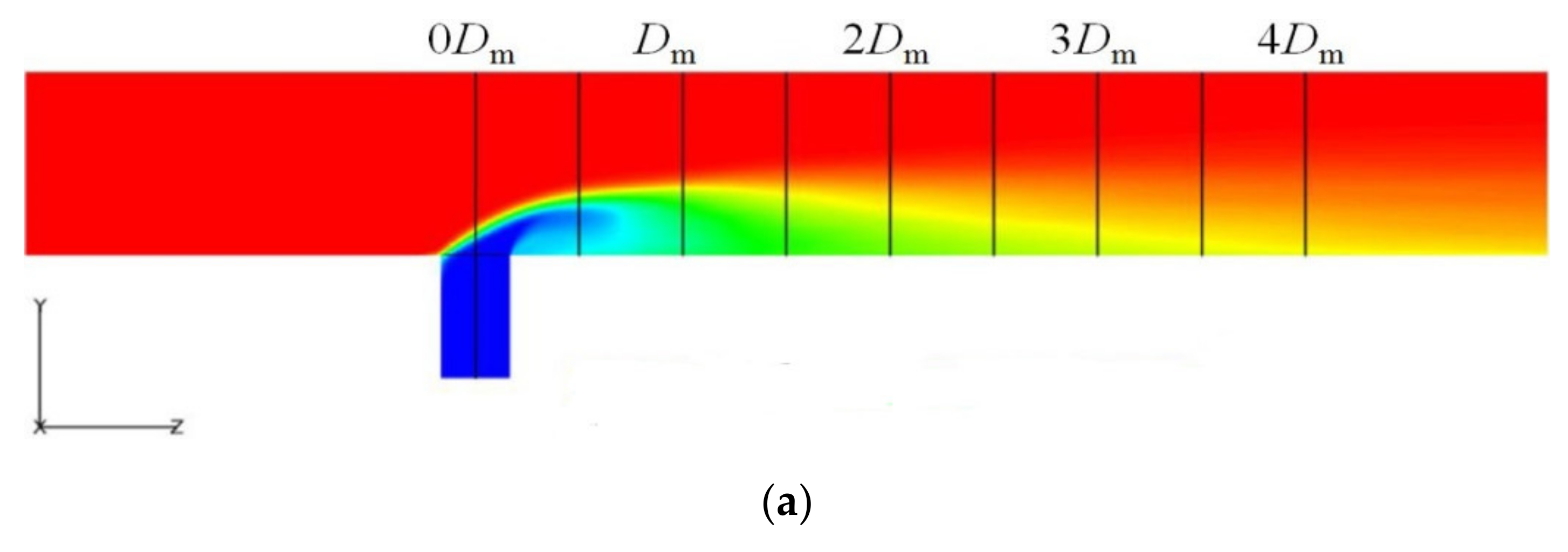
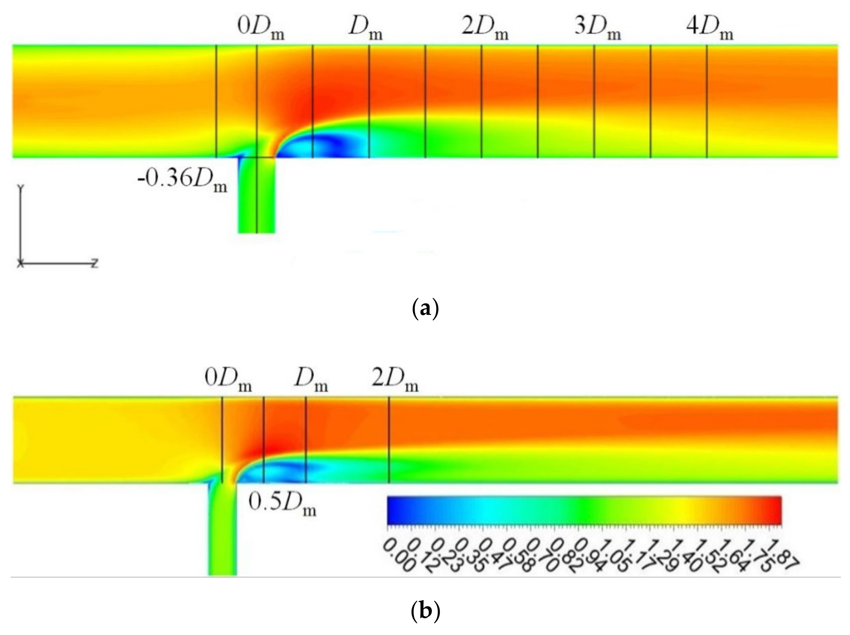
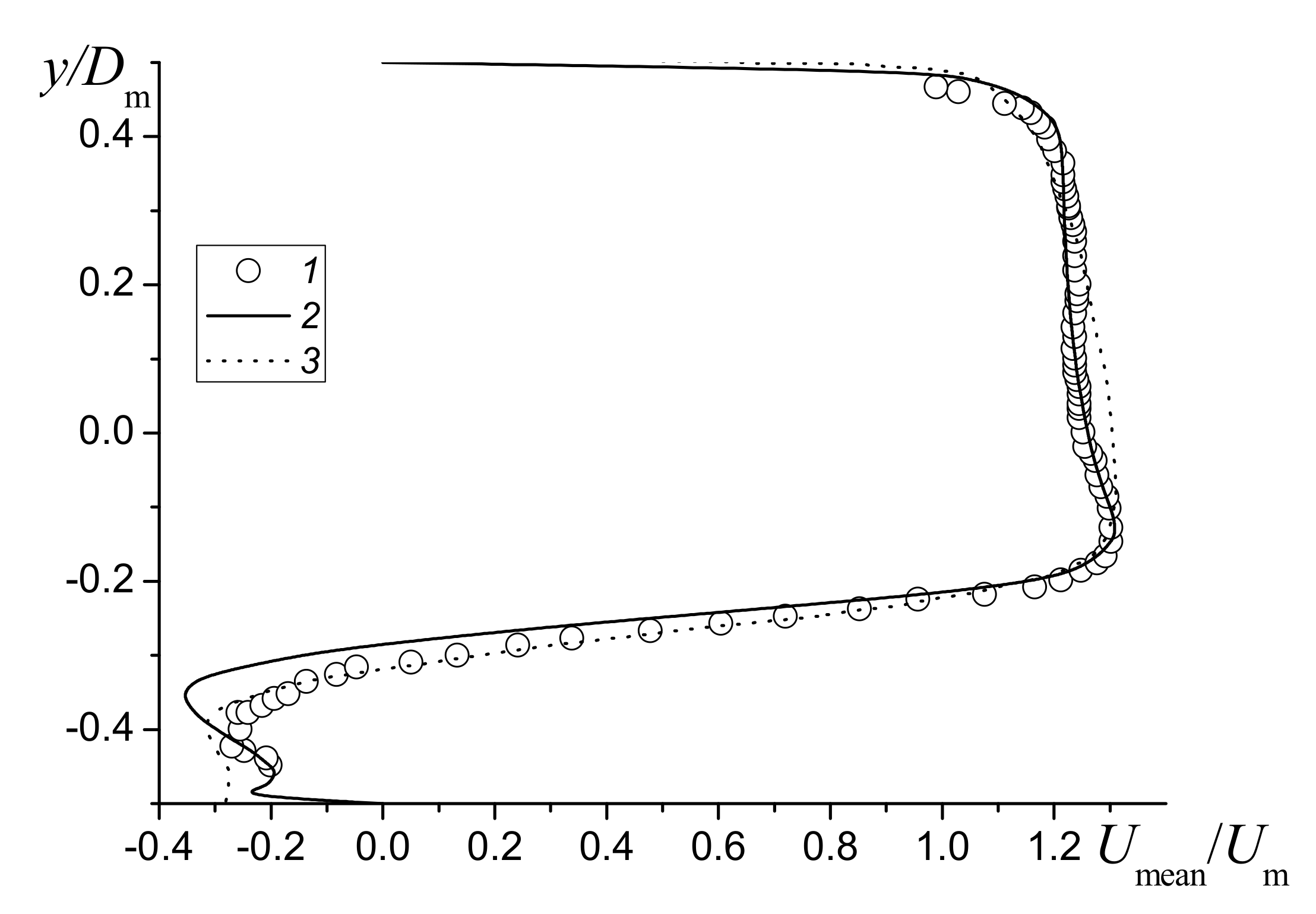
Within the near-wall jet regime (Table 1), the jet with a temperature Tb is issuing from the socket into the main flow with a temperature Tm and presses it to the channel wall (Figure 3). In the main pipe downstream, the socket flow with the temperature Tb near the wall is gradually mixed with the flow with the temperature Tm in the main pipe. As seen from Figure 3, within this mixing regime, the RANS mixing results show that mixing occurs more slowly in comparison to the LES results [11]. In the RANS approach, the mixing zone is longer. This fact is confirmed by the dimensionless temperature distribution T* = (T−Tb)/(Tm−Tb) in the channel cross-sections at the distances of 0.5Dm and 1.0Dm downstream behind the socket center (Figure 4). The RANS results are compared to the LES results [9]. As seen from the temperature distributions in the channel cross-sections, the low-temperature region is maintained up to the distance x = 1.0Dm. It is found that the region sizes are smaller than those determined by the LES approach [9]. For a more detailed comparison, Figure 5 presents the averaged temperature profile along the vertical line at a distance of 0.5Dm behind the socket center. The abscissa axis is the dimensionless temperature T* and the ordinate axis—the dimensionless distance y/Dm, where y is taken along the vertical line mentioned above.
The experimental and numerical simulation results illustrate that the dimensionless temperature is practically constant in the main flow (y/Dm > −0.1) and rapidly decreases at the mixing layer boundary (−0.3 < y/Dm< −0.1). The temperature near the pipe wall slightly increases due to the fact that the recirculating flow captures some part of the immiscible medium with a higher temperature from the mixing layer (Figure 3). Figure 5 demonstrates that regardless of the numerical simulation approach used in this region, the predicted results and the WATLON data [10] do not agree—the RANS approach underestimates the temperature value, while the LES approach overestimates it. As described in [19], the LES results obtained with the use of different computational meshes were not practically different and demonstrated the overestimated temperature value near the main pipe wall. The LES results [20,21], when the numerical simulation approach used the near-wall functions and the computational meshes were formed with the thermal boundary layer resolution, also showed the overestimated temperature value near the main pipe wall.
Thus, regardless of the numerical simulation approach (RANS or LES), the problem remains how to adequately describe the temperature field at intense mixing of heat carrier flows. However, from the viewpoint of solving thermal fatigue, the LES overestimation of the temperature value can be considered as a positive factor since it allows predicting the start of critical phenomena with some time.
The averaged velocity distribution in Figure 6 demonstrates that near the surface of the main pipe downstream behind the socket, there are formed the stagnation zone of the flow issuing from the socket and the recirculating flow zone that somewhat presses the main pipe flow, which results in its velocity increase. The latter is seen in the RANS and LES approaches.
Figure 7 presents the profile of the dimensionless averaged longitudinal velocity Umean/Um along the vertical line at the distance z = 0.5Dm downstream behind the socket center. The abscissa axis is the dimensionless averaged velocity and the ordinate axis—the dimensionless distance y/Dm. The overestimated velocity value is seen in the main pipe center. It is obtained by the LES approach [11] in comparison to the WATLON data [10] and by the RANS approach. The LES results [20] showed the same behavior, assuming that the numerically simulated profile depends on the velocity profile assigned as the boundary conditions at the main pipe inlet. One of the possible reasons for differences between experiment and numerical simulation was that in the experiment, the flow at the pipe inlet was not fully developed (the velocity profile is flat). Apparently, this explains the agreement between the RANS results and the experimental data for y/Dm > −0.1 since, when the RANS approach was used in our numerical simulation, the velocity was constant at the computational domain inlet.
The flow velocity in the WATLON experiment [10] is almost constant for the main flow (y/Dm > −0.1) and decreases in the direction to the wall, at which the socket is placed (Figure 7). In this region, the LES results well enough show both this tendency and the change in the numerical velocity unlike the RANS approach where its value is underestimated. Here, apparently the LES advantage is seen from the viewpoint of reflecting the complex local unsteady vortex structure of the flow unlike the RANS approach that only yields the averaged flow pattern.
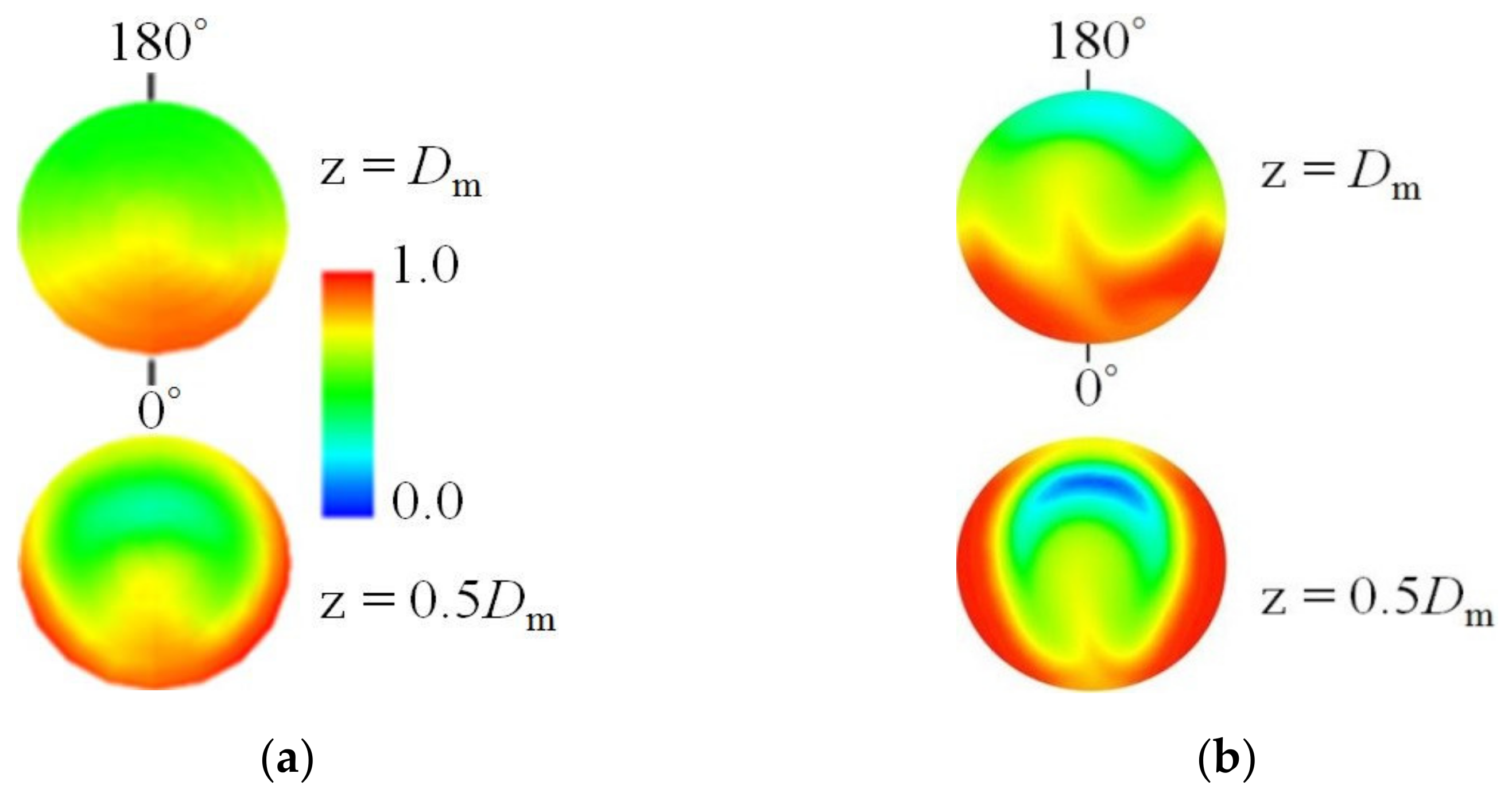
In case of a deflecting jet, mixing occurs in a peculiar cocoon shaped as a divergent cone downstream behind the socket when a significant change in the dimensionless temperature is not seen near the pipe wall (Figure 8). The dimensionless temperature mainly changes in the central part of the flow. Moreover, as shown in Figure 8b, the RANS results qualitatively agree with the LES results.
In case of an impact jet, the heat carrier issuing from the socket reaches the opposite wall of the main pipe (Table 1). This is evident of the fact that already at a sufficiently small distance in the main pipe downstream behind the socket, a mixed medium is formed at z = 0.5Dm (Figure 9). At that, in the main pipe downstream, unlike the near-wall jet, the decreased temperature region exists in the upper part of the main pipe (Figure 9). Flows with different temperatures are mixed sufficiently intensely already in the cross-section z = 1.0Dm, the main pipe has a pronounced near-wall increased temperature region, a mixing layer, and a decreased temperature region. As shown in Figure 9b, the RANS results demonstrate a mixing delay in comparison to the LES results [6].
2.2. Stuttgart Experiment Simulation
The static pressure in the computational domain was 75 bars. The values of the temperature Tm and the mass flowrate Qm were assigned at the main pipe inlet. To assign turbulence characteristics, the turbulence fluctuation level Tu = 1% and the hydraulic diameter dhyd m = Dm. The values of the temperature Tb and the mass flowrate Qb were assigned at the socket inlet in order to predetermine the turbulence characteristics in the socket—the turbulence fluctuation level Tu = 1% and the hydraulic diameter dhyd b = Db. The mass flowrate ratio is Qm/Qb = 1/4. Soft boundary conditions were assigned at the computational domain outlet. The T-junction walls were assumed to be thermally insulated. The heat carrier thermal/physical properties (viscosity coefficient, thermal conductivity) were assigned in the form of temperature-dependent piece-linear functions. The temperature- and pressure-dependent density was assigned [13].
The behavior of the flow at the starting length of the main pipe from the inlet opening to a place of supplying heat carrier from the socket determines the mixing character in the T-junction.
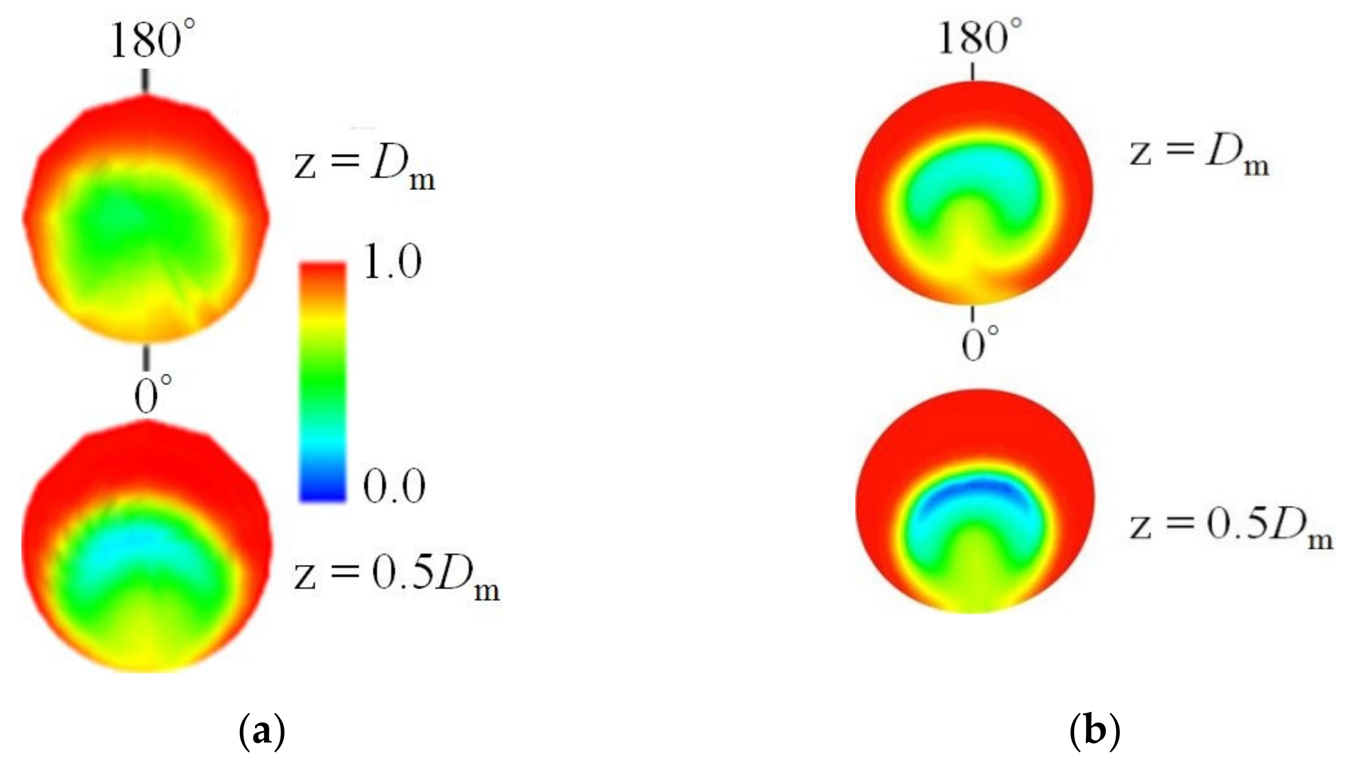
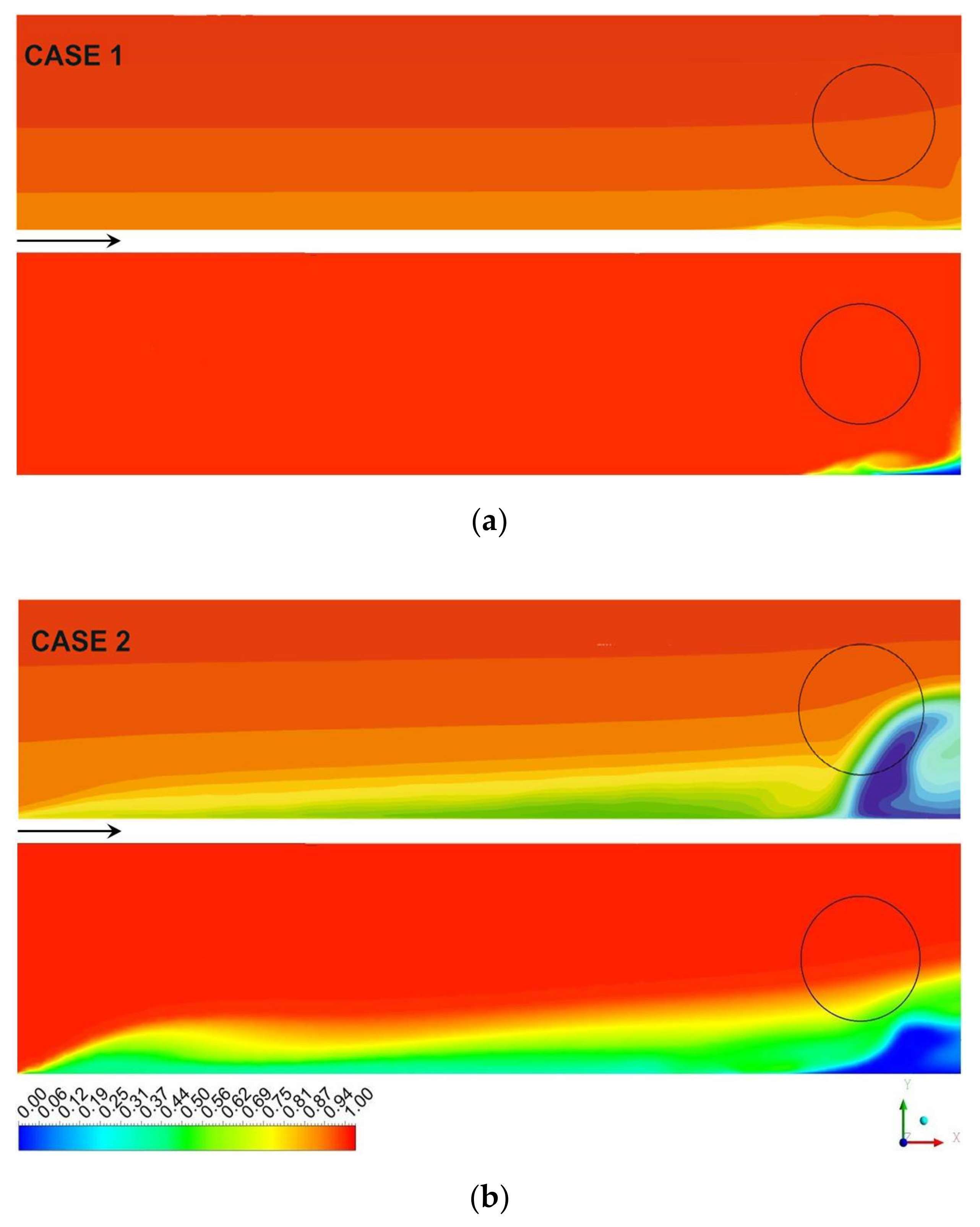
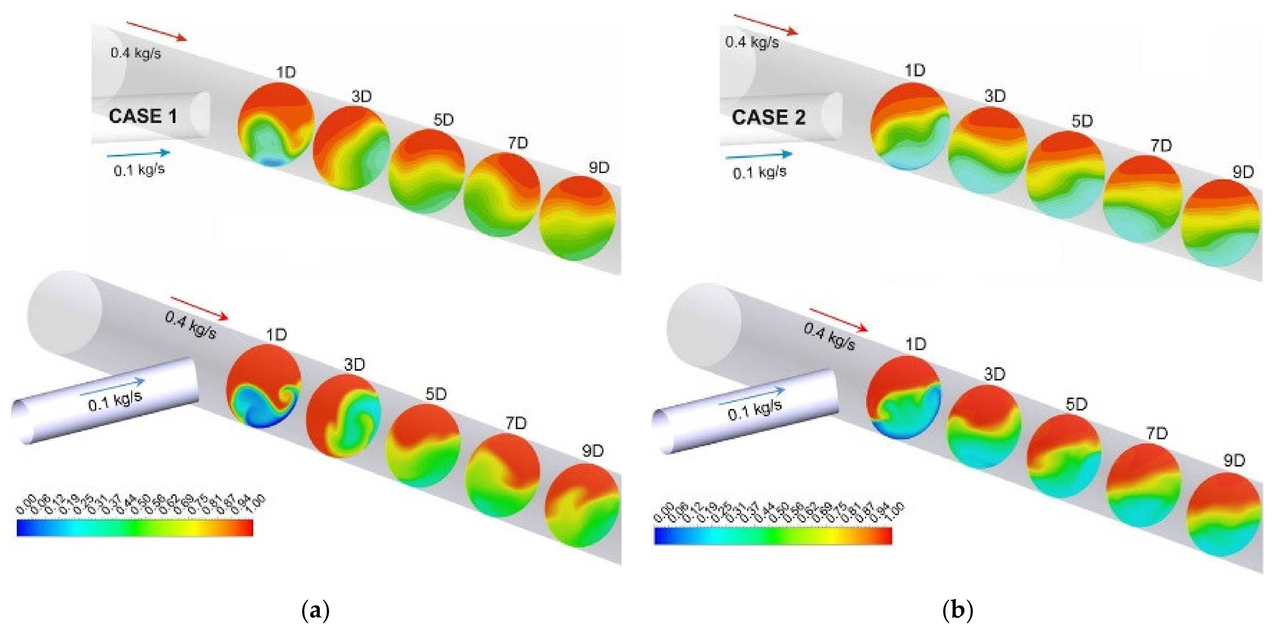
Figure 10 shows the distribution of the normalized temperature T* = (T−Tb)/(Tm−Tb). The hot heat carrier flow in the main pipe keeps constant temperature (ST1, Table 2), except for a small area where a cold heat carrier overflows from the socket into the main pipe.
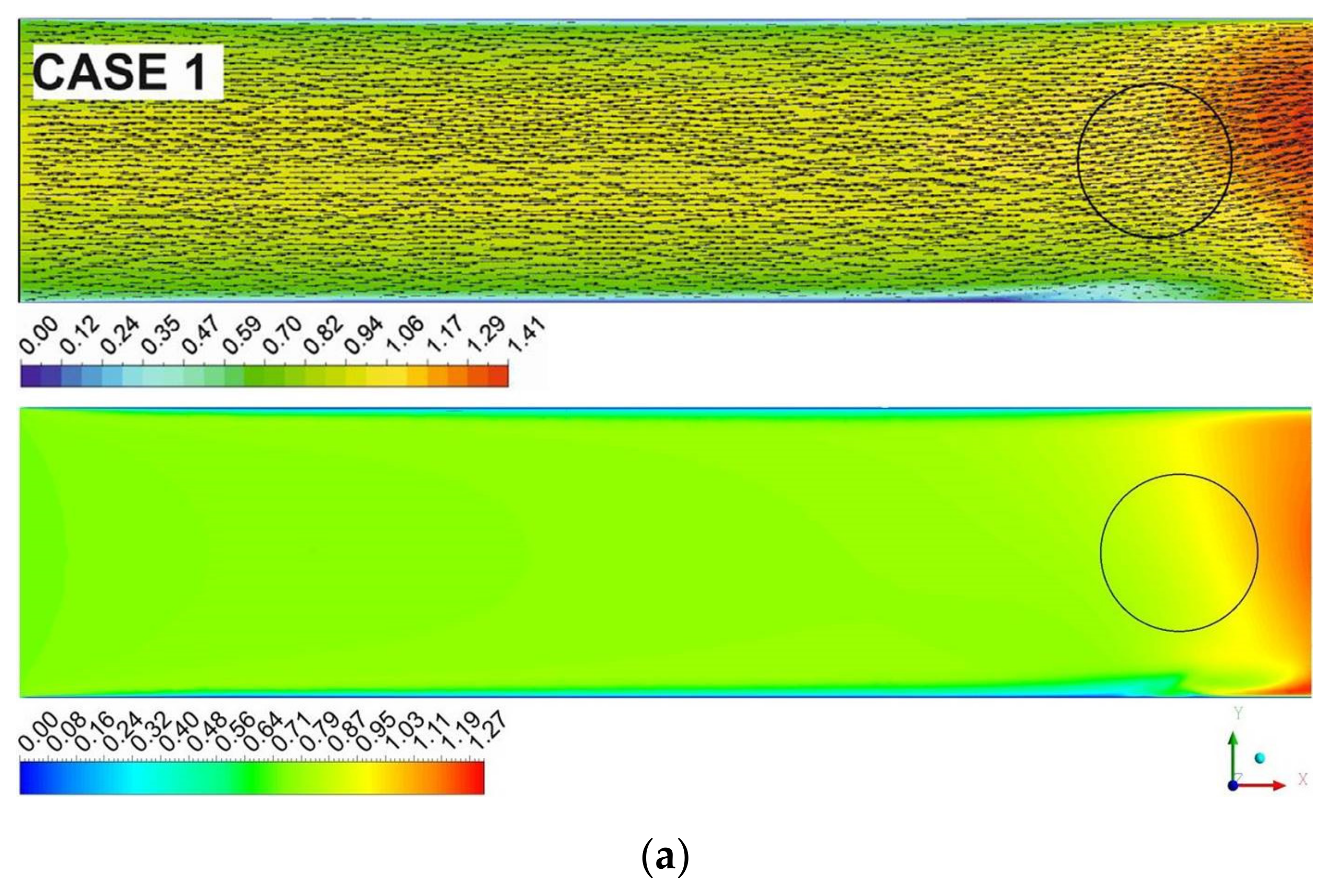
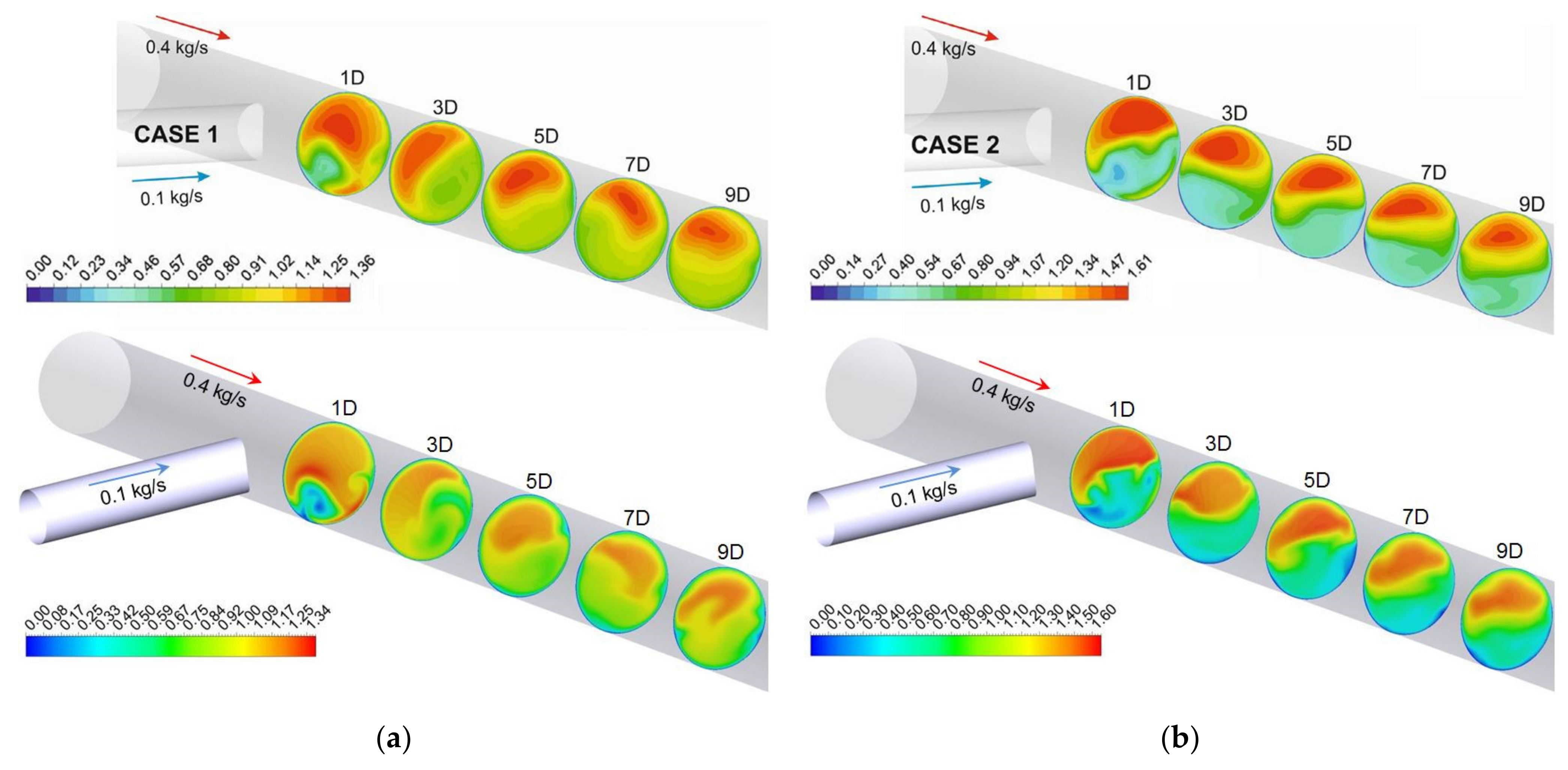
The overflow occurs at a distance of 0.55Dm from the central axis of the socket (Figure 10) due to a density difference between the main pipe flow and the socket flow. It is 3%. This results in the formation of the recirculating flow zone as shown in Figure 11 illustrating the distribution of the dimensionless velocity .
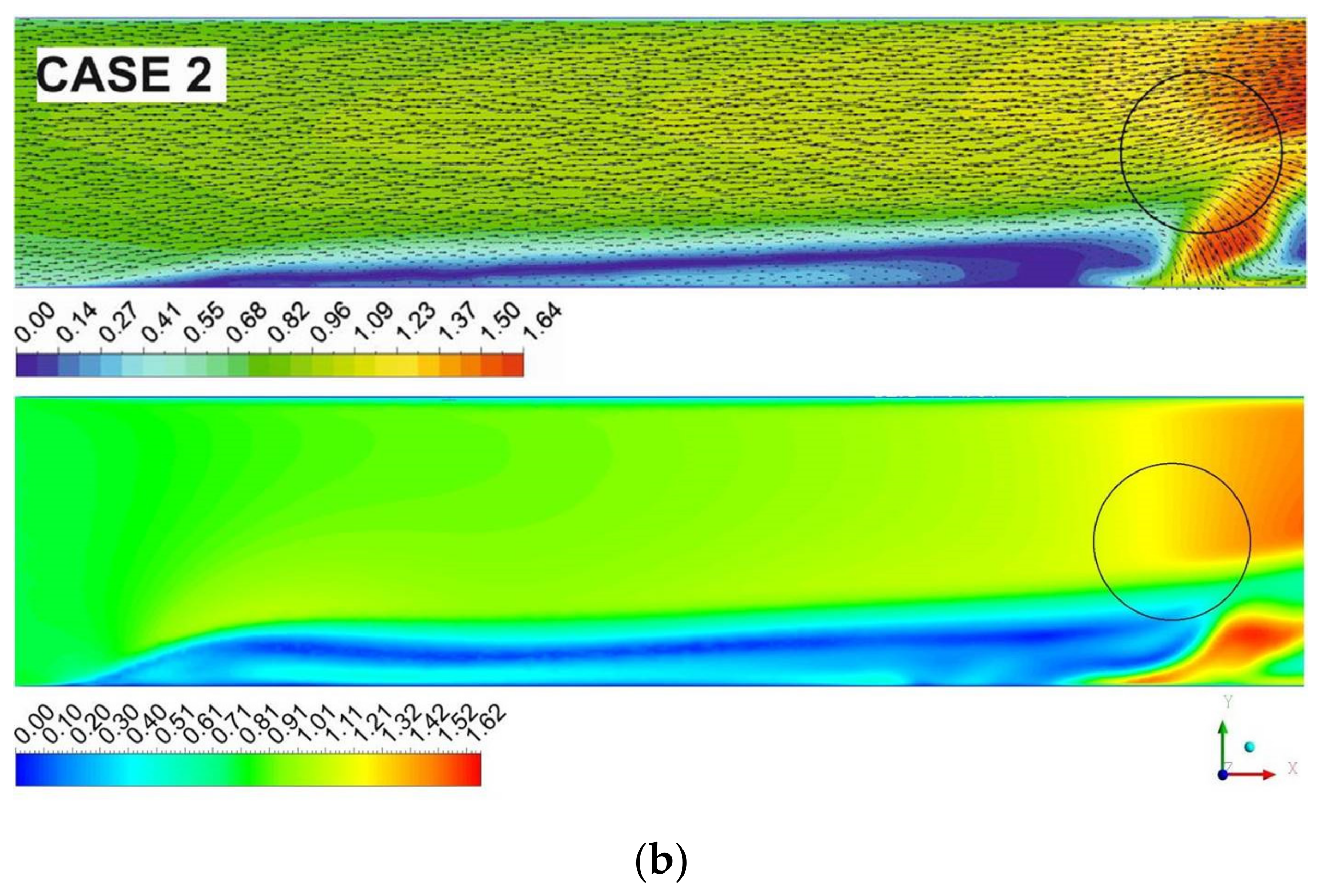
With the mass flowrate ratio in the main pipe and in the socket invariable, increasing the temperature drop to ΔT = 143° due to a heat carrier temperature growth in the main pipe causes a large overflow of a cold heat carrier from the socket into the main pipe at a distance of about 3.57Dm from the central axis of the socket (Figure 10). It can be assumed that the main reason for this phenomenon is associated with increasing the relative density ρm/ρb by 10% (it is more than a three-fold increase in comparison to Case 1 (regime ST1).
The low velocity of a cold heat carrier issuing from the socket results in separating the flow in the T-junction, when one part of the flow moves upstream and the other—downstream. This causes the size of the recirculating flow zone to increase (Figure 11).
The mixing process in the T-junction is affected by the size of a forming recirculating flow zone. In experiment, the wire mesh sensor located upstream behind the mixing zone of the T-junction did not detect any penetration of the cold flow in the case of ST2 at the distance x = −3.53Dm, while the thermocouples located at the distance x = −1.6Dm detected the outflow of the cold heat carrier [12]. A maximum distance, at which the cold heat carrier outflow occurs (hence, a maximum size of the recirculating flow zone), is between the thermocouples and the wire mesh sensor. As shown in Figure 12, the LES and RANS predictions also indicate a distance of the cold heat carrier outflow that is close to the position of the wire mesh sensor [12].
Based on the fact that the Reynolds number ratio Rem/Reb = 6.6 (Case 1, regime ST1) and Rem/Reb = 12.3 (Case 2, regime ST2), the near-wall jet is formed in the T-junction, i.e., the flow downstream is not completely mixed and stratified by temperature (accordingly, by density). What is more, hot and cold heat carrier flows are only mixed downstream in some part of the main pipe. This results in forming three separate regions, the state of which can be identified as follows. The first region is the hot heat carrier area upstream ahead of the mixing zone; the heat carrier is not mixed in this area. The second region is the mixed flow area significantly downstream behind the mixing zone. The third region is located between the first and second flow areas, where stratified layers undergo separation, and hence it is characterized by high temperature gradients. The behavior of the stratified flow within the regimes ST1 and ST2 differ sharply from each other (Figure 12). Within the regime ST1 the sharp temperature gradients are formed when cold and hot heat carrier flows are mixed.
In Case 2 (regime ST2), hot and cold heat carriers are quickly stratified, the cold heat carrier settles at the bottom of the main pipe and the hot heat carrier is located at the top of the pipe. Such a behavior is characteristic of the flow in the whole part of the main pipe behind the mixing zone. Such a difference in the flow behavior is most likely associated with the buoyancy forces, the manifestation of which becomes more significant with increase in the temperature drop ΔT between the inlets of the main pipe and the socket, which yields a very fast flow separation by to density.
Figure 13 shows the distribution of the average velocity U* in different sections of the main pipe downstream behind the T-junction. In the mixing region, the highest velocities are seen at the top of the main pipe behind the mixing zone where a hot heat carrier of lower density flows, not mixing. The lower velocities are observed at the bottom of the main pipe where a mixed heat carrier flows and intermediate velocities are seen in the vicinity of the mixing layer. The liquid velocity at the bottom of the main pipe in Case 1 (regime ST1) is higher in comparison to Case 2 (regime ST2). This may be associated with the cold heat carrier outflow into the main pipe upstream from the T-junction in Case 2 (regime ST2) (Figure 13 and Figure 14), which decelerates the flow of the hot heat carrier moving in the main pipe to the mixing zone. Heat and mass transfer between cold and hot heat carriers in the mixing zone may cause low be velocities at the bottom of the pipe in Case 2 (regime ST2) in comparison to Case 1 (regime ST1). As mentioned above, the temperature fluctuation in the flow in Case 1 (regime ST1), where the buoyancy effects play no significant role in comparison to Case 2 (regime ST2), for which at a small distance from the mixing zone, hot and cold heat carriers are sharply separated, the temperature fluctuations are significantly lower, and the buoyancy effects play a decisive role.
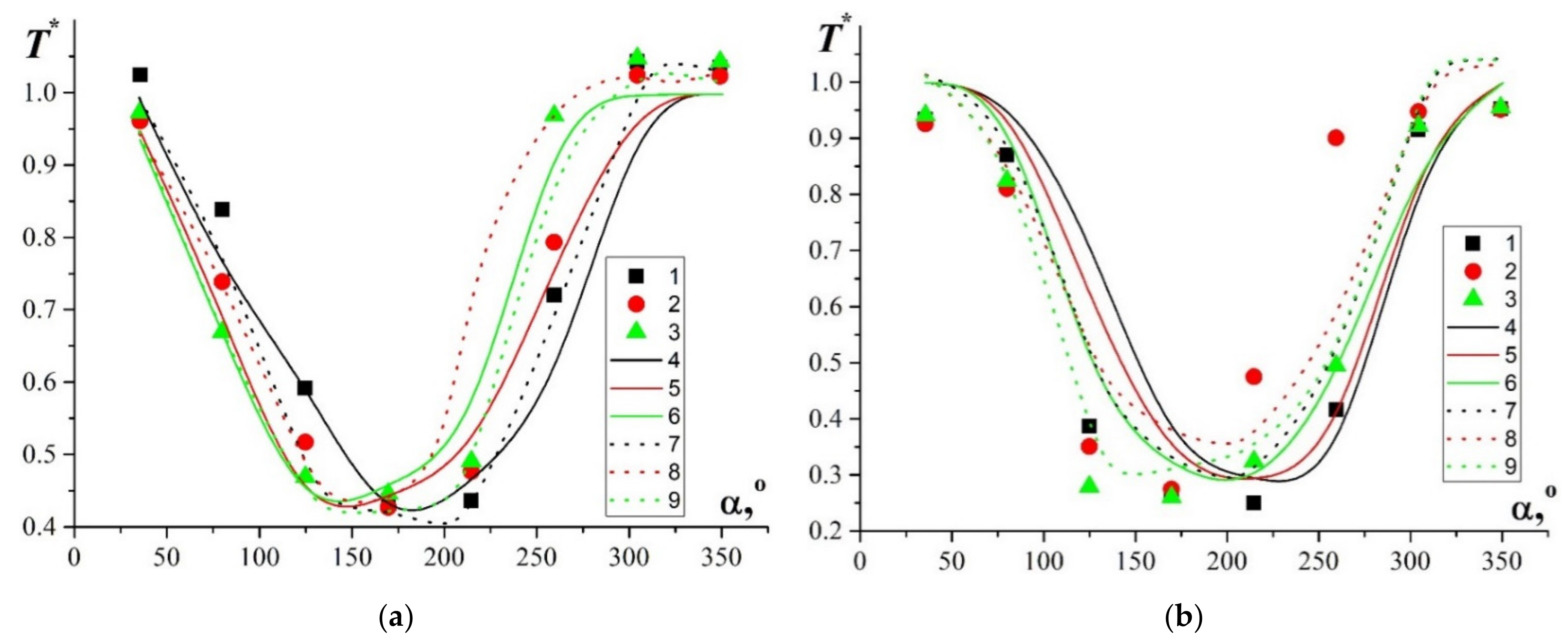
In experimental study [12], the flow thermocouple were located at the distance x = 5Dm; x = 6Dm; x = 9.7Dm и x = 10.7Dm, while the wall thermocouples—at the distances x = 5.5Dm and x = 10.2Dm. Figure 14a and Figure 15a show the averaged temperature distribution in the near-wall region registered with the thermocouples in the cross-section of the main pipe for Case 1 (ST1) and compare the LES and RANS results.
The temperature, close in value to the hot heat carrier temperature (Tm = 358 K), was observed at the top of the main pipe on the angular coordinates (α = 9.5°, 35.5°, 54.5°, 305.5°, 324.5°, 350.5°), confirming that heat carriers in this region are not practically mixed. The lowest averaged temperatures are registered at the top of the pipe (α = 170.5°, 215.5°, 189.5°, 234.5°). Thus, a difference in the averaged temperature profile form between the sections x = 5Dm to 6Dm and x = 9.7Dm to 10.7Dm can be explained by the flow fluctuations caused by averaged temperature variations. Bearing in mind the data in Figure 14a and Figure 15a, we can judge about the position of the mixing layer that separates hot and cold heat carriers. For example, it can be located near α = 80.5° or α = 125.5° and 260.5° between the sections x = 5Dm and x = 6Dm, since sharp temperature gradients are observed in the vicinity of the angular positions.
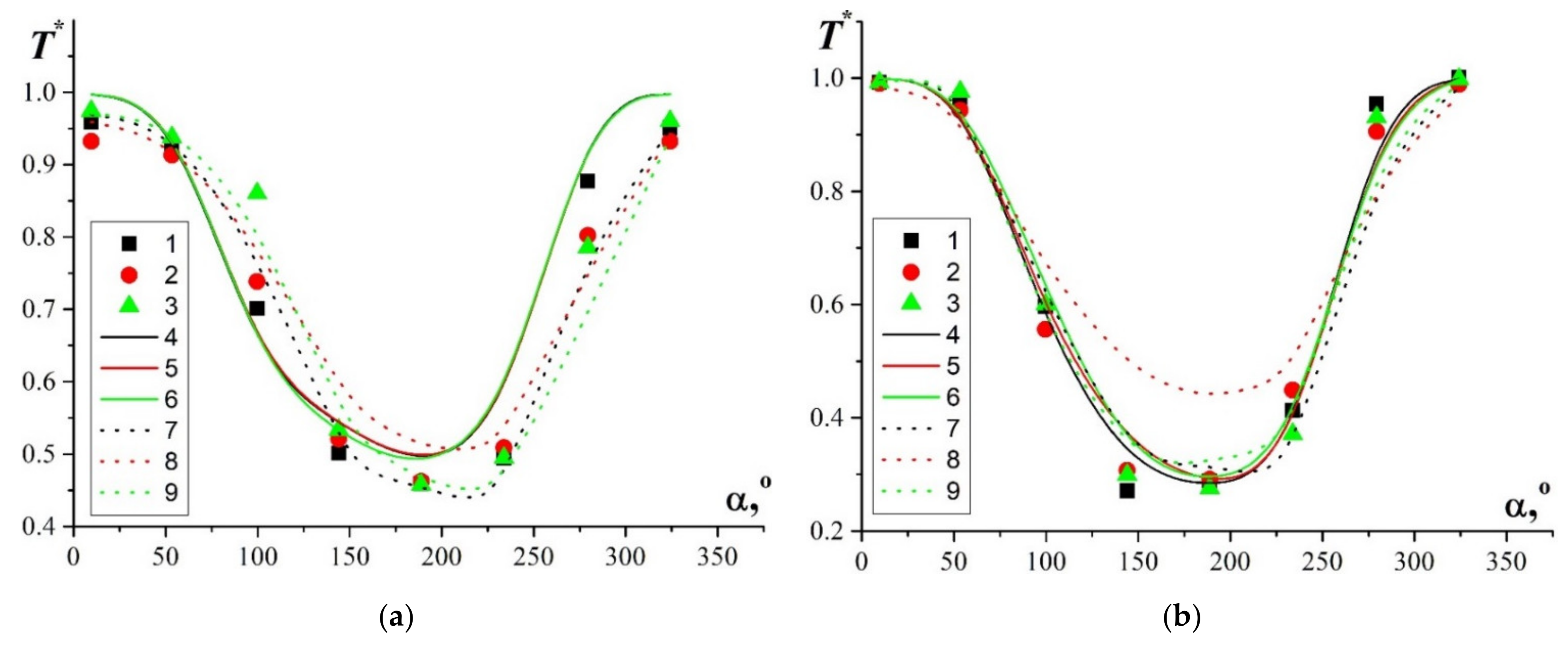
Figure 14b and Figure 15b present the averaged temperature distribution in Case 2 (regime ST2) obtained experimentally, as well as by the LES and RANS approaches. The presented results show the averaged temperature profile form is similar at different locations of thermocouples. This is evident of the fact that a strongly stratified flow, in which the buoyancy effects play a decisive role, is formed in the main pipe downstream behind the mixing zone. The presence of maximum averaged temperature values shows that hot and cold heat carrier flows are not mixed; they are observed near the upper wall of the main pipe on the angular coordinates (α = 9.5°, 35.5°, 324.5°, 350.5°). Minimum averaged temperature values are seen at the top of the pipe (α = 144.5°, 170.5°, 189.5°, 215.5°).
The mixing layer in Case 2 (regime ST2) can be located between the angular coordinates α = 80.5° and 125.5° (on the left side of the main pipe) and 260.5° (on the right side of the main pipe) between the sections x = 5Dm and x = 6Dm. The temperature drop in the flow between the upper wall of the main pipe (α = 350.5°) and the lower wall (α = 170.5°) is of about 40° in the section x = 5Dm in Case 1 (regime ST1), reaching 61% of the initial temperature drop ΔT = Tm−Tb = 65°. In Case 2 (regime ST2), the temperature drop between the upper and lower walls of the main pipe in the section x = 5Dm increases and is 108.5° according to the LES approach and is about 101° according to the RANS approach. It is about 76% (LES) and 71% (RANS) of the initial temperature drop ΔT = Tm−Tb = 143°.
Determining the temperature drop in the stratified flow in the main pipe downstream behind the T-junction is important from the viewpoint of occurring local thermal stresses in the pipe itself that can give rise to deformation and cracking [22]. The visual observations made during the experimental study [12] showed that the pipe did not undergo deformation in Case 1 (regime ST1), while in Case 2 (regime ST2), the construction bent slightly. It should be noted that the LES and RANS predictions are close to the experimental results.
3. Conclusions
The numerical simulation approach of heat carrier mixing regimes in the T-junction shows that the RANS approach is beneficial for a qualitative flow analysis to obtain relatively agreed averaged velocity and temperature. Moreover, traditionally, the RANS approach only predicts the averaged temperature distribution. This mathematical model did not consider the temperature fluctuation variations [23] important for the thermal fatigue task. It should also be emphasized that unlike the LES approach, the steady RANS approach cannot express a local flow structure in intense mixing zones. Nevertheless, apparently the adopted RANS approach should be used for assessing the quality of computational meshes, boundary conditions with the purpose to take LES for further numerical simulation.
The results on heat carrier mixing in the T-junction at significant drops of temperature and pressure greater than atmospheric can be generalized as follows:
- In both the considered cases, hot and cold heat carrier are not fully mixed. The flow in the main pipe is stratified downstream behind the T-junction. To get more full mixing, it is necessary to increase the velocity (Reynolds number) at the inlets of the main pipe and the socket, which will result in realizing another flow regime in the main pipe (impact jet or deflecting jet [9]);
- The behavior of the flow stratified by temperature is determined by the temperature drop between mixing flows. Temperature fluctuations have maximum values near the mixing layer. In Case 1 (regime ST1), there appears an unstable- stratified flow with significant temperature fluctuations. In Case 2 (regime ST2), the stable-stratified flow is observed, in which the buoyancy effects are decisive;
- The LES and RANS results on the temperature in the near-wall region of the flow and in the flow behind the T-junction agree with the experimental data obtained with the use of the mesh sensor and thermocouples. The comparison of the experimental data and the LES and RANS results shows that RANS can be utilized for qualitative and quantitative descriptions of mixing processes in the main pipe behind the T-junction.
Author Contributions
Conceptualization, A.D.C., Y.V.Z. and I.A.P.; methodology, Y.V.Z., T.A.B. and A.S.; numerical simulations, T.A.B., Y.V.Z. and A.S.; numerical data analysis and preparation formal analysis, T.A.B., Y.V.Z. and I.A.P.; data curation, Y.V.Z. and A.D.C.; writing—original draft preparation, T.A.B., Y.V.Z. and A.S.; writing—review and editing, I.A.P. and A.D.C.; supervision, A.D.C. and I.A.P.; project administration, Y.V.Z., A.D.C. and I.A.P. All authors have read and agreed to the published version of the manuscript.
Funding
The work was financially supported by the Ministry of Education and Science of the Russian Federation as part of the fulfillment of obligations to fulfill obligations under the Agreement 075-03-2020-051/3 dated of 09.06.20 and Belarusian Republican Foundation for Fundamental Research (project F21MS-011).
Institutional Review Board Statement
Not applicable.
Informed Consent Statement
Not applicable.
Data Availability Statement
Not applicable.
Conflicts of Interest
The authors declare no conflict of interest.
References
- Belov, V.V.; Pergamenshchik, B.K. Krupnye avarii na TES i ikh vliyanie na komponovochnye resheniya glavnykh korpusov [Large-scale Accidents at Thermal Power Plants (TPPs) and Their Influence on Equipment Layouts inside Main Buildings]. Vestn. MGSU Proc. Mosc. State Univ. Civ. Eng. 2013, 4, 61–69. [Google Scholar] [CrossRef]
- Birger, I.-P. Calculation of the Strength of Machine Parts: Handbook, 4th ed.; Birger, I.-P., Shorr, B.F., Iosilevich, G.V., Eds.; Mashinostroyeniye: Moscow, Russia, 1993; 640p. [Google Scholar]
- Zhukovsky, N.-X. About Water Hit in Water Pipes—Moscow; GITTL: Leningrad, Russia, 1949; 104p. [Google Scholar]
- Assessment of Computational Fluid Dynamics (CFD) for Nuclear Reactor Safety Problems; Nuclear Energy Agency, Committee on the Safety of Nuclear Installations: Paris, France, 2008; NEA/CSNI/R (2007) 13; 180p.
- Chapuliot, S.; Gourdin, C.; Payen, T.; Magnaud, J.; Monavon, A. Hydro-thermal-mechanical analysis of thermal fatigue in a mixing tee. Nucl. Eng. Des. 2005, 235, 575–596. [Google Scholar] [CrossRef]
- McDevitt, M.; Hoehn, M.; Childress, T.; McGill, R. Analysis and impact of recent U.S. thermal fatigue operating experience. In Proceedings of the Fourth International Conference on Fatigue of Nuclear Reactor Components, Seville, Spain, 28 September–1 October 2015; No. 28. [Google Scholar]
- Braillard, O.; Edelin, D. Advanced experimental tools designed for the assessment of the thermal load applied to the mixing tee and nozzle geometries in the PWR plant. In 2009 1st International Conference on Advancements in Nuclear Instrumentation, Measurement Methods and their Applications; IEEE: Marseille, France, 2009; pp. 1–7. [Google Scholar]
- Zhou, M.; Kulenovic, R.; Laurien, E. Experimental investigation on the thermal mixing characteristics at a 90° T-Junction with varied temperature differences. Appl. Therm. Eng. 2018, 128, 1359–1371. [Google Scholar] [CrossRef]
- Kamide, H.; Igarashi, M.; Kawashima, S.; Kimura, N.; Hayashi, K. Study on mixing behavior in a tee piping and numerical analyses for evaluation of thermal striping. Nucl. Eng. Des. 2009, 239, 58–67. [Google Scholar] [CrossRef]
- Igarashi, M.; Tanaka, M.; Kawashima, S.; Kamide, H. Experimental study on fluid mixing for evaluation of thermal striping in T-pipe junction. In Proceedings of the 10th International Conference on Nuclear Engineering, Arlington, MA, USA, 14–18 April 2002; pp. 383–390. [Google Scholar]
- Utanohara, Y.; Miyoshi, Y.K.; Nakamura, A. Conjugate numerical simulation of wall temperature fluctuation at a T-junction pipe. Bulletin of the JSME. Mech. Eng. J. 2018, 5, 1–23. [Google Scholar] [CrossRef] [Green Version]
- Selvam, P.K.; Kulenovic, R.; Laurien, E.; Kickhofel, J.; Prasser, H.-M. Thermal mixing of flows in horizontal T-junctions with low branch velocities. Nucl. Eng. Des. 2017, 332, 32–54. [Google Scholar] [CrossRef]
- Vilner, Y.M.; Kovalev, Y.T.; Nekrasov, B.B. Handbook for Hydraulics, Hydraulic Machines and Hydraulic Drives; Vysheishaya Shkola: Minsk, Russia, 1976; 416p. [Google Scholar]
- Zhou, M.; Kulenovic, R.; Laurien, E. T-junction experiments to investigate thermal-mixing pipe flow with combined measurement techniques. Appl. Therm. Eng. 2019, 150, 237–249. [Google Scholar] [CrossRef]
- Menter, F.R.; Kuntz, M.; Langtry, R. Ten years of industrial experience with the SST turbulence model. In Turbulence, Heat and Mass Transfer 4; Hanjalic, K., Nagano, Y., Tummers, M., Eds.; Begell House, Inc.: Danbury, CT, USA, 2003. [Google Scholar]
- Sosinovich, V.-P. Turbulent Motion of Incompressible Media; Luikov, A.V., Ed.; Heat and Mass Transfer Institute of NAS of Belarus: Minsk, Belarus, 2007; 189p.
- Patankar, S.V. Computation of Conduction and Duct Flow Heat Transfer; CRC Press: Maple Grove, MN, USA, 1991; 370p. [Google Scholar]
- Aksenov, A.A.; Zhluktov, S.V.; Shmelev, V.V.; Shaporenko, E.V.; Shepelev, S.F.; Rogozhkin, S.A.; Krylov, A.N. Numerical investigations of mixing non-isothermal streams of sodium coolant in T-branch. Comput. Res. Modeling 2017, 9, 95–110. [Google Scholar] [CrossRef] [Green Version]
- Utanohara, Y.; Nakamura, A.; Miyoshi, K.; Kasahara, N. Numerical simulation of long-period fluid temperature fluctuation at a mixing tee for the thermal fatigue problem. Nucl. Eng. Des. 2016, 305, 639–652. [Google Scholar] [CrossRef]
- Nakamura, A.; Ikeda, H.; Qian, S.; Tanaka, M.; Kasahara, N. Benchmark simulation of temperature fluctuation using CFD for the evaluation of the thermal load in a T-junction pipe. In Proceedings of the seventh Korea-Japan Symposium on Nuclear Thermal Hydraulics and Safety, Chuncheon, Korea, 14–17 November 2010. Paper No. N7P-0011. [Google Scholar]
- Tanaka, M.; Ohshima, H.; Monji, H. Thermal mixing in T-junction piping system concerned with high-cycle thermal fatigue in structure. J. Nucl. Sci. Technol. 2010, 47, 790–801. [Google Scholar] [CrossRef]
- Kweon, H.D.; Kim, J.S.; Lee, K.Y. Fatigue design of nuclear class 1 piping considering thermal stratification. Nucl. Eng. Des. 2008, 238, 1265–1274. [Google Scholar] [CrossRef]
- Qian, S.; Kanamaru, S.; Kasahara, N. High-accuracy CFD prediction methods for fluid and structure temperature fluctuations at T-junction for thermal fatigue evaluation. Nucl. Eng. Des. 2015, 288, 98–109. [Google Scholar] [CrossRef]
- Isaev, A.; Kulenovic, R.; Eckart, L. Experimental investigation on isothermal stratified flow mixing in a horizontal T-junction. Atw Int. Z. Kernenerg. 2016, 61, 621–624. [Google Scholar]
- Evrim, C.; Chu, X.; Silber, F.E.; Isaev, A.; Weihe, S.; Laurien, E. Flow features and thermal stress evaluation in turbulent mixing flows. Int. J. Heat Mass Transf. 2021, 178, 121605. [Google Scholar] [CrossRef]
- Dmitriev, S.M.; Dobrov, A.A.; Legchanov, M.A.; Khrobostov, A.E. Modeling of Coolant Flow in the Fuel Assembly of the Reactor of a Floating Nuclear Power Plant Using the Logos CFD Program. J. Eng. Phys. Thermophys. 2015, 88, 1297–1303. [Google Scholar] [CrossRef]
Figure 1.
T-junction.

Figure 2.
CAD model cross section (a) and computational mesh fragment in the mixing zone of the T-junction (b).
Figure 2.
CAD model cross section (a) and computational mesh fragment in the mixing zone of the T-junction (b).

Figure 3.
Averaged temperature distribution (in C deg) in the middle section of the T-junction at Rem/Reb = 5.76 obtained by the following approaches: (a) LES [11]; (b) RANS.
Figure 3.
Averaged temperature distribution (in C deg) in the middle section of the T-junction at Rem/Reb = 5.76 obtained by the following approaches: (a) LES [11]; (b) RANS.


Figure 4.
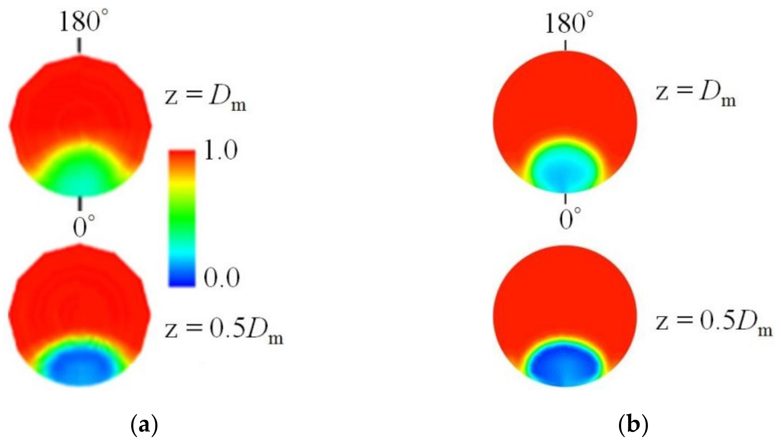
Distribution of the dimensionless temperature T* at Rem/Reb = 5.76: (a) LES [9]; (b) RANS.
Figure 4.
Distribution of the dimensionless temperature T* at Rem/Reb = 5.76: (a) LES [9]; (b) RANS.

Figure 5.
Distribution of the dimensionless temperature T* in the section at the distance z = 0.5Dm behind the socket center at Rem/Reb = 5.76: (1) WATLON data [10]; (2) RANS; (3) LES [11].

Figure 6.
Absolute averaged velocity distribution (in m/s) in the middle section of the T-junction at Rem/Reb = 5.76: (a) LES [11]; (b) RANS.
Figure 6.
Absolute averaged velocity distribution (in m/s) in the middle section of the T-junction at Rem/Reb = 5.76: (a) LES [11]; (b) RANS.

Figure 7.
Distribution of the dimensionless velocity Umean /Um in the section at the distance behind the socket center for Rem/Reb = 5.76: (1) WATLON experiment [10]; (2) RANS; (3) LES [11].

Figure 8.
Distribution of the dimensionless temperature T* at Rem/Reb = 1.81: (a) LES [9]; (b) RANS.
Figure 8.
Distribution of the dimensionless temperature T* at Rem/Reb = 1.81: (a) LES [9]; (b) RANS.

Figure 9.
Distribution of the dimensionless temperature T* at Rem/Reb = 0.91: (a) LES [9]; (b) RANS.
Figure 9.
Distribution of the dimensionless temperature T* at Rem/Reb = 0.91: (a) LES [9]; (b) RANS.

Figure 10.
Distribution of the dimensionless temperature T* in the middle plane of the T-junction (black circle—inlet opening of the socket): (a)—ST1, Table 2 (top figure—LES results [12], bottom figure—RANS results); (b)—ST2, Table 2 (top figure—LES results [12], bottom figure—RANS results).

Figure 11.
Distribution of the dimensionless velocity U* in the middle plane of the T-junction (black circle—inlet opening of the socket): (a)—ST1, Table 2 (top figure—LES results [12], bottom figure—RANS results); (b)—ST2, Table 2 (top figure—LES results [12], bottom figure—RANS results).


Figure 12.
Variation of the dimensionless temperature T* in different sections downstream behind the mixing zone: (a)—ST1, Table 2 (top figure—LES results [12], bottom figure—RANS results); (b)—ST2, Table 2 (top figure—LES results [12], bottom figure—RANS results).

Figure 13.
Distribution of the dimensionless velocity U* in different sections downstream behind the mixing zone: (a)—ST1, Table 2 (top figure—LES results [12], bottom figure—RANS results); (b)—ST2, Table 2 (top figure—LES results [12], bottom figure—RANS results).

Figure 14.
Profiles of the dimensionless temperature T* obtained experimentally [12] (symbols), by the LES approach [12] (dashed lines) and by the RANS approach (solid lines): regime ST1 (a), regime ST2 (b): 1, 4, 7—Section 5Dm; 2, 5, 8—Section 5.5Dm; 3, 6, 9—Section 6Dm.

Figure 15.
Profiles of the dimensionless temperature T* obtained experimentally [12] (symbols), by the LES approach [12] (dashed lines) and by the RANS approach (solid lines): regime ST1 (a), regime ST2 (b): 1, 4, 7—Section 9.7Dm; 2, 5, 8—Section 10.2Dm; 3, 6, 9—Section 10.7Dm.


| Regime | Rem/Reb | Mm/Mb | Flow Visualization |
|---|---|---|---|
| Near-wall jet | Rem/Reb > 2.36 | Mm/Mb > 1.35 |  |
| Deflecting jet | 1.2 < Rem/Reb< 2.36 | 0.35 < Mm/Mb < 1.35 |  |
| Impact jet | Rem/Reb < 1.2 | Mm/Mb < 0.35 |  |
Publisher’s Note: MDPI stays neutral with regard to jurisdictional claims in published maps and institutional affiliations. |
© 2021 by the authors. Licensee MDPI, Basel, Switzerland. This article is an open access article distributed under the terms and conditions of the Creative Commons Attribution (CC BY) license (https://creativecommons.org/licenses/by/4.0/).
Share and Cite
MDPI and ACS Style
Baranova, T.A.; Zhukova, Y.V.; Chorny, A.D.; Skrypnik, A.; Popov, I.A. Non-Isothermal Vortex Flow in the T-Junction Pipe. Energies 2021, 14, 7002. https://0-doi-org.brum.beds.ac.uk/10.3390/en14217002
AMA Style
Baranova TA, Zhukova YV, Chorny AD, Skrypnik A, Popov IA. Non-Isothermal Vortex Flow in the T-Junction Pipe. Energies. 2021; 14(21):7002. https://0-doi-org.brum.beds.ac.uk/10.3390/en14217002
Chicago/Turabian StyleBaranova, Tatyana A., Yulia V. Zhukova, Andrei D. Chorny, Artem Skrypnik, and Igor A. Popov. 2021. "Non-Isothermal Vortex Flow in the T-Junction Pipe" Energies 14, no. 21: 7002. https://0-doi-org.brum.beds.ac.uk/10.3390/en14217002
Note that from the first issue of 2016, this journal uses article numbers instead of page numbers. See further details here.