
Quantitative Performance Comparison of Thermal Structure Function Computations


1
Faculty of Electrical Engineering, South Westphalia University of Applied Sciences, 59494 Soest, Germany
2
Fraunhofer Application Center for Inorganic Phosphors, Branch Lab of Fraunhofer Institute for Microstructure of Materials IMWS, 59494 Soest, Germany
*
Author to whom correspondence should be addressed.
Energies 2021, 14(21), 7068; https://0-doi-org.brum.beds.ac.uk/10.3390/en14217068
Submission received: 30 September 2021
/
Revised: 21 October 2021
/
Accepted: 22 October 2021
/
Published: 28 October 2021
(This article belongs to the Special Issue Latest Advances in Electrothermal Models II)
Abstract
:The determination of thermal structure functions from transient thermal measurements using network identification by deconvolution is a delicate process as it is sensitive to noise in the measured data. Great care must be taken not only during the measurement process but also to ensure a stable implementation of the algorithm. In this paper, a method is presented that quantifies the absolute accuracy of network identification on the basis of different test structures. For this purpose, three measures of accuracy are defined. By these metrics, several variants of network identification are optimized and compared against each other. Performance in the presence of noise is analyzed by adding Gaussian noise to the input data. In the cases tested, the use of a Bayesian deconvolution provided the best results.
1. Introduction
In the field of thermal management, detailed finite element models and multiphysics simulations are developed to predict the behavior of a system with high accuracy. From these detailed descriptions, reduced-order models are constructed which guide thermal design and system-level integration [1].
However, measurements on real devices can never be replaced completely. There are a number of aspects in which physical measurements and simulations complement and depend on each other. These include the development of new materials, the quantification of their physical parameters, the verification of simulation results, as well as quality assurance in production processes.
A commonly applied method for thermal measurements is network identification by deconvolution [2,3,4] as first described by Vladimir Székely and Tran Van Bien of the Budapest University of Technology in 1988 [5] and standardized by JEDEC Committee JC15 in 2010 [6]. In this method, the dynamic properties of a one-dimensional heat path are derived from a transient thermal measurement, i.e., the temperature response to a step in heating power. After a transition to the logarithmic time domain, the temperature response is differentiated, from which the time constant spectrum is computed by numerical deconvolution. Finally, a Foster-to-Cauer transformation is performed to obtain the thermal structure function.
As network identification by deconvolution is a very noise sensitive procedure, effort is put into finding an optimal measurement setup and evaluation procedure. In this context, Lasance and Poppe state that the “ curves must be extremely noise free” ([7], p. 129) and the JEDEC standard notes that the method is “extremely sensitive to noise” ([6], p. 16). To achieve a high accuracy, good performance in the steps of differentiation and deconvolution is crucial [8]. In particular for short times, noise is detrimental to the accuracy of the method. In an attempt to address this issue from the experimental side, Schmid et al. have developed a time-saving algorithm for transient thermal analysis which reduces noise in the measured data via repeated measurements [9]. On the algorithmic side, the effects of noise on time constant spectra and structure functions have been considered [10]. However, the question remains as to which the most suitable procedure is. Responding to these challenges, a method for verifying the accuracy of implementations was presented by Szalai and Székely [11]. While this procedure allows to evaluate the general suitability of an implementation, an absolute measure of accuracy is needed for a fair comparison between the different approaches.
For differentiation, the JEDEC standard recommends a straight line fit [6]. Schmid et al. used a Savitzky-Golay filter of second order [12]. In this work, a Savitzky-Golay filter of first order with an adaptive step size subroutine is used. For the evaluation of thermal transients, the evaluation software of the Simcenter T3Ster Master by Mentor Graphics is commonly used. The details of its implementation are, however, not disclosed.
For deconvolution, Fourier deconvolution as well as Bayesian deconvolution have been discussed [13,14]. In the literature, much effort has been put into developing good window functions [15]. The JEDEC standard describes a deconvolution based on a Fermi filter [6]. Székely found success using a Gauss filter [16]. In principle, Wiener optimal filtering is also possible [17]. An approach using inverse filtering is presented by Székely [18].
A detailed analysis of Bayesian deconvolution is given in [19,20,21] and a derivation specifically for network identification by deconvolution can be found in [22]. The use of Bayesian deconvolution is reported by Ezzahri and A. Shakouri [2]. For the main iteration, Székely recommends using approximately 1000 steps [13,23]. The same number is used by Schmid et al. [9]. Pareek et al. use 1000 to 2000 steps [14].
For the Foster-to-Cauer transformation, three methods are reported [24]. An approach using polynomial long division is described in detail in [25]. A state-space method is laid out in [26]. A tridiagonalization method is presented by Codecasa in [24].
Modern approaches offer the possibility to bypass the deconvolution step [27]. An approach by Codecasa uses a multi-point moment matching technique [28] to calculate the Foster network from the thermal response. In this way, it is also possible to generate the thermal structure function directly from the spatial distribution of the thermal resistances and the thermal capacitances of a three-dimensional thermal model.
In this work, a suggestion is made how to rank accuracies of thermal structure functions and time constant spectra resulting from a specific implementation of network identification by deconvolution. Typical variants of the method are systematically analyzed and improved with respect to their accuracy.
2. Network Identification by Deconvolution
2.1. Linear Responses
This section gives an overview of key mathematical relations in the context of network identification by deconvolution. For an introduction into the subject, the reader is referred to [6,7]. A detailed theoretical treatment is given in [13]. Detailed information on transmission lines and structure functions can be found in [29].
A transient thermal measurement captures the thermal response of a device to a step in heating power. Here, the concept of linear time-invariant systems plays a major role for the mathematical description. In this formalism, an input function is related to an output function via the impulse response, , which reflects the behavior of the system. The heating power, , serves as input function, while the temperature curve, is the output function. Both are connected by a convolution equation,
where is the equilibrium temperature. The impulse response is defined as the reaction of the system to a delta-function input. It is connected to the step response, , via differentiation,
In the context of transient thermal measurements, the step response, , is also called thermal impedance, . It is defined as
where P describes the height of the power step.
2.2. Thermal Equivalence Networks
The goal of network identification by deconvolution is to derive a thermal equivalence network for a given driving point impedance of , where s is the complex frequency. The resistances and capacitances of the electric network should relate to the thermal resistances and thermal capacitances of the system. The theory of network identification by deconvolution provides analytical equations to directly obtain the parameters of an equivalence network of a Foster-type RC-ladder, see Figure 1. However, these resistances and capacitances, denoted and , are not directly related to their thermal counterparts in the device. For this reason, the Foster-type network is subsequently converted to a Cauer-type network, see Figure 2.
The impedance, , of a Foster-type RC network with n stages is a sum of impedances of each stage,
This function has poles at . Here, , are the time constants, which are defined as
Its step response, , can be directly constructed from the network and amounts to
For easier generalization to the infinite case, , (6) is presented in integral form. It is formulated with the help of the time constant spectrum, , which is a sum of delta functions,
2.3. Logarithmic Time
For practical computations, it is easier to work in logarithmic time, z, and to use the logarithmic time constant, , which are defined as
Often, and are suppressed, as it is done below. Using these definitions, the logarithmic thermal impedance, , is defined as
and the logarithmic impulse response, , follows as
In logarithmic time, the time constant spectrum (7), becomes
2.4. Network Identification
To identify the thermal resistances and capacitances of the Cauer network, see Figure 2, the Foster network has to be calculated first. The components of the Cauer network are directly related to the time constant spectrum. The integral in (13) can be interpreted as a convolution of the time constant spectrum, ,
with the weight function, ,
From the logarithmic time constant spectrum, the resistances, , and capacitances, , of the Foster network follow,
Here, is the logarithmic time constant discretized with step size , where .
Next, the Foster network has to be converted to a Cauer network. To differentiate the components, Cauer resistances, , and Cauer capacitances, , are denoted with a prime. In the Cauer network, the capacitances are directly connected to the grounded lower port, i.e., these resistances and capacitances directly correspond to thermal counterparts. As described in the introduction, there are several ways to perform this conversion.
Finally, the Cauer network is related to the physical structure of the system. To this end, the linear thermal resistances density, , and the linear thermal capacitances density are defined. Here, x is the one-dimensional spatial coordinate of the physical system. The cumulative resistance, , and the cumulative capacitance, , are the antiderivatives, i.e.,
The thermal structure function is then defined as the function, , and constitutes the final result of the network identification by deconvolution, see [29].
2.5. Inverse Calculations
In network identification by deconvolution, a thermal equivalence network is constructed from a thermal impedance, whereas in inverse calculation, the thermal impedance is derived from a given thermal network. From a uniform transmission line with total resistance and total capacitance , the input impedance, , can be calculated according to
Here, is the load impedance, which is either zero or equal to the input impedance of the previous transmission line in case of connected transmission lines.
Given the impedance of the transmission line, the logarithmic time constant spectrum is its the imaginary part, ℑ, along the negative real axis,
To avoid poles in the impedance, see (4), a small angle, , is introduced into the complex frequency, i.e., the integration path is slightly rotated into the complex plane,
3. Methodology
3.1. Measures of Accuracy
To evaluate the accuracy of an implementation for network identification, a reference structure is defined. It has the form of a chain of uniform transmission lines, here called a piecewise uniform structure function. Then, an inverse calculation is performed to obtain its thermal impedance. Starting from this impedance, network identifications are performed with the goal to reconstruct the reference structure.
For the evaluation, the measure of accuracy plays a central role. The goal is to find two suitable functionals, one for measuring the accuracy of the time constant spectrum and one for the structure function. These should adequately measure the degree of similarity between the theoretical ideal and a given solution.
One challenge in comparing two different time constant spectra is the sharpness of the peaks. When comparing two spectra, it is not sufficient to directly integrate the difference between them via an -norm. Due to the sharpness of the peaks, the overlap between two adjacent peaks is small and their relative distance outside the overlap is not taken into account. In addition, the height of the peaks in the theoretical ideal depends on the angle . The goal is to develop a measure which is insensitive to the value of .
For this reason, the integrated time constant spectrum, , is considered,
In this form, the delta-function-like peaks of a theoretical time constant spectrum become a staircase function. By using , the total area under the curve is measured and can be included in the evaluation. For the time constant spectrum in particular, this is important as the area under the curve is proportional to the total resistance.
Thus, the measure of accuracy for the time constant spectrum, , has the form of an -norm of the difference between the integrated theoretically ideal and the reconstructed time constant spectra,
As time constant spectra are equal to zero in the limit , the integration boundaries are set to infinity. The -norm is chosen, as opposed to an absolute norm, to weight larger differences stronger than smaller ones. A large difference can occur for example if the location of a peak is shifted on the -axis. To calculate the difference between two spectra, possibly one of the spectra has to be interpolated to match the other.
For the structure function, , a more complex functional is necessary. This is mainly because of the following three challenges that arise when quantitatively comparing structure functions.
Firstly, the cumulative thermal capacity, , typically spans several orders of magnitude. For this reason, it is often plotted on a logarithmic axis.
Secondly, the structure function is constructed from the thermal resistances and capacities provided by the Foster-to-Cauer transformation. Consequently, two structure functions will not have exactly the same set of on which they are defined. This means that the starting and end points of two structure functions will not generally be the same, i.e., either one of the structure function has to be extrapolated or the other has to be truncated.
This is important as, thirdly, structure functions calculated via Bayesian deconvolution or Fourier deconvolution typically feature a smeared-out divergence at the end. This is a real disadvantage of these methods. Nevertheless, the measure of accuracy should not consider whether the structure function ends at, for example, or .
Given these challenges, the following measure of accuracy for the structure function, , is defined,
The logarithm is used to not overemphasize deviations at high values of . In the logarithm, is to be inserted in units of . It also helps to not disproportionately punish a structure function with a long divergence. For the same reasons, all structure functions are truncated at . The integration limits, and , are defined as
For the lower boundary, the theoretical structure function defines the limit of integration and the recovered structure function is truncated or extrapolated accordingly. For the upper boundary, the limit is defined by the recovered structure function. Alternatively, the divergence of the recovered structure function could be extrapolated to match the theoretical structure function. However, this would make the divergence the dominant contribution to . In contrast, extrapolating the theoretical structure function is not an issue, as it does not diverge. Truncating the recovered structure function when the theoretical structure function ends puts a bias into to favor divergences at higher in the recovered structure function, i.e., it is biased to overestimate the total thermal resistance. For this reason, the limits are defined as in (26).
Measuring the accuracy of structure functions via (25) means that the absolute accuracy of the total thermal resistance is not reflected in . The upper integration limit is defined by the point of the divergence via (26). Only the shape of the divergence is taken into account and not its relative position. For these reasons, an additional measure of accuracy is used to characterize the total resistance belonging to the recovered structure function. The difference in total resistance, , is calculated by comparing the theoretically expected resistance to as defined in (26),
3.2. Computations in the Presence of Noise
To evaluate the robustness of the algorithms when confronted with real measurement data, Gaussian noise is added to the theoretically calculated thermal impedance. The standard deviation of the noise, , is defined via the signal-to-noise ratio, , and the asymptotic value of the thermal impedance, ,
As the results should not depend on a single noise pattern only, many noisy thermal impedances are generated and solved. For the calculations, 2000 randomly generated noisy thermal impedances are evaluated. As a result, the median over the 2000 solutions is calculated and compared on the basis of the accuracy measures (24), (25), and (27).
For the impulse response, the median is calculated point by point as all discrete z-values, on which the solutions are defined, are identical. For the structure function, each solution is interpolated and, if necessary, also extrapolated to guarantee that they all have the same domain. The normalized structure functions are then averaged by pointwise calculation of the median. Finally, the divergence of the median structure function is truncated as described above.
The time constant spectra, however, are not averaged directly, as the result would be highly biased towards zero. Here, the integrated time constant spectrum is computed for each realization. The set of resulting integrated time constant spectra is then averaged. For the sake of accuracy comparisons, this is acceptable, since only integrated time constant spectra are compared finally.
The Gaussian distributed random numbers are generated via the default random number generator available in NumPy 1.19.2. To guarantee repeatability, for each of the 2000 realizations an individual fixed seed is used. For repeated calculations with different parameters, for instance in the case of the same calculation with two different signal-to-noise ratios, identical noise patterns are generated, but with different standard deviations. In any case, averaging over 2000 repetitions makes the median almost completely independent of a particular set of noise patterns.
4. Algorithmic Details
4.1. Optimal Regression Filtering
In this work, the network identification by deconvolution relies on a regression filter to reduce noise in the thermal impedance and to calculate its derivative. Explicitly, the data are smoothed by so-called LOcally Weighted Scatterplot Smoothing (LOWESS). During derivation, it is important to choose an appropriate window length that balances the bias-variance tradeoff. For this, Stein’s Unbiased Risk Estimate (SURE) is applied. The idea is based on a paper by Krishnan and Seelamantula [30]. Here, an adaptation suitable for network identification is presented. One challenge lies in taking into account the unevenly spaced measurement data.
The measurement of a noisy signal is described by assuming an underlying real signal, , which, is subject to (Gaussian) noise, , such that the observed values are . Here, i enumerates the data points and each set, , has an associated logarithmic time, . From the set of all measurement points, , a small subset, , is taken to approximate the true value, , at a specific location. The size of the interval measured in logarithmic time, z, is called window length, L, while the window size, N, denotes the number of data points. To achieve a good fit, the window length has to be chosen carefully. A polynomial of low order is fitted to via a least squares regression that generates a prediction, , of . Where possible, is located in the center of , such that lies inside . In practice, approximating via a polynomial of first order has performed best. The derivative of is then simply approximated by its gradient.
Each data point is assigned a weight inversely proportional to the local density of points, such that sparse sections of the signal are not underrepresented. In addition, the data points are weighted according to their distance, , from via a tricubic weight function , which is defined as
Next, the adaptive step size subroutine is outlined. As is unknown in practice, the magnitude of the error made with the prediction is unknown. The estimated error of the prediction, , of is called the statistical risk. Here, it is calculated via SURE [30]. According to SURE the associated risk, , is
In practice, the measurement points are not evenly spaced which is a requirement for fast Fourier transformations and Bayesian deconvolution. Thus, the derivative is not evaluated at , but at a location nearby, . The set of new logarithmic time provides a constant spacing . The number of points, , to be chosen for the new grid is considered below. On the basis of (30), the optimal window length is chosen by searching for an L that minimizes . In practice, the search is limited to an interval, , within reasonable boundaries. Freely choosing L at each often leads to an oscillating behavior, i.e., additional high frequency noise in the output. The initial window length at is freely chosen in the interval , while in each subsequent step the window length is incremented or decremented by . At each the risk associated with the window lengths , L, and is calculated and the window lengths adjusted accordingly. In addition, this update scheme limits the amount of computational work introduced by the adaptive step size subroutine.
4.2. Deconvolution
For Bayesian deconvolution, a prior distribution equal to the impulse response, , is used, but a constant prior distribution is also possible. Beyond a certain number of iteration steps the results are independent of the prior distribution.
In Fourier space, the impulse response becomes a function of the logarithmic frequency, . A filter, , is applied to each component of the spectrum. As defined in (31), components beyond the cut-off frequency, , are suppressed. Frequencies between and are damped according to the window function, , in question,
For the window function, many forms are possible, a selection of which is tested in the following. The support of the filter function, i.e., its non-zero components, forms an array with entries that are numbered from zero to from negative to positive, . For each window function, the width of the window is controlled via , which is realized in the form of in the definitions below. The Nuttall window, the Hann window, and the rectangular window are defined as
The Nuttall window is a sum-of-cosines window with specific numerical prefactors developed by Nutall [31]. The Gaussian window has an additional parameter, , which is restricted to ,
The Fermi window is a special case as it does not use a finite cut-off frequency, . Instead, it uses two parameters, and , which control its width and slope. The support is the entire spectrum,
The right-hand side of (36) is more stable for small .
5. Reference Structures
For comparison, three reference structures are defined. Their theoretical transient thermal impedances serve as artificial measurement data. The difference between the original and the recovered time constant spectrum and the structure function is quantified to give a measure of accuracy. The structures are defined as piecewise uniform structure functions consisting of several sections with thermal resistances and capacitances.
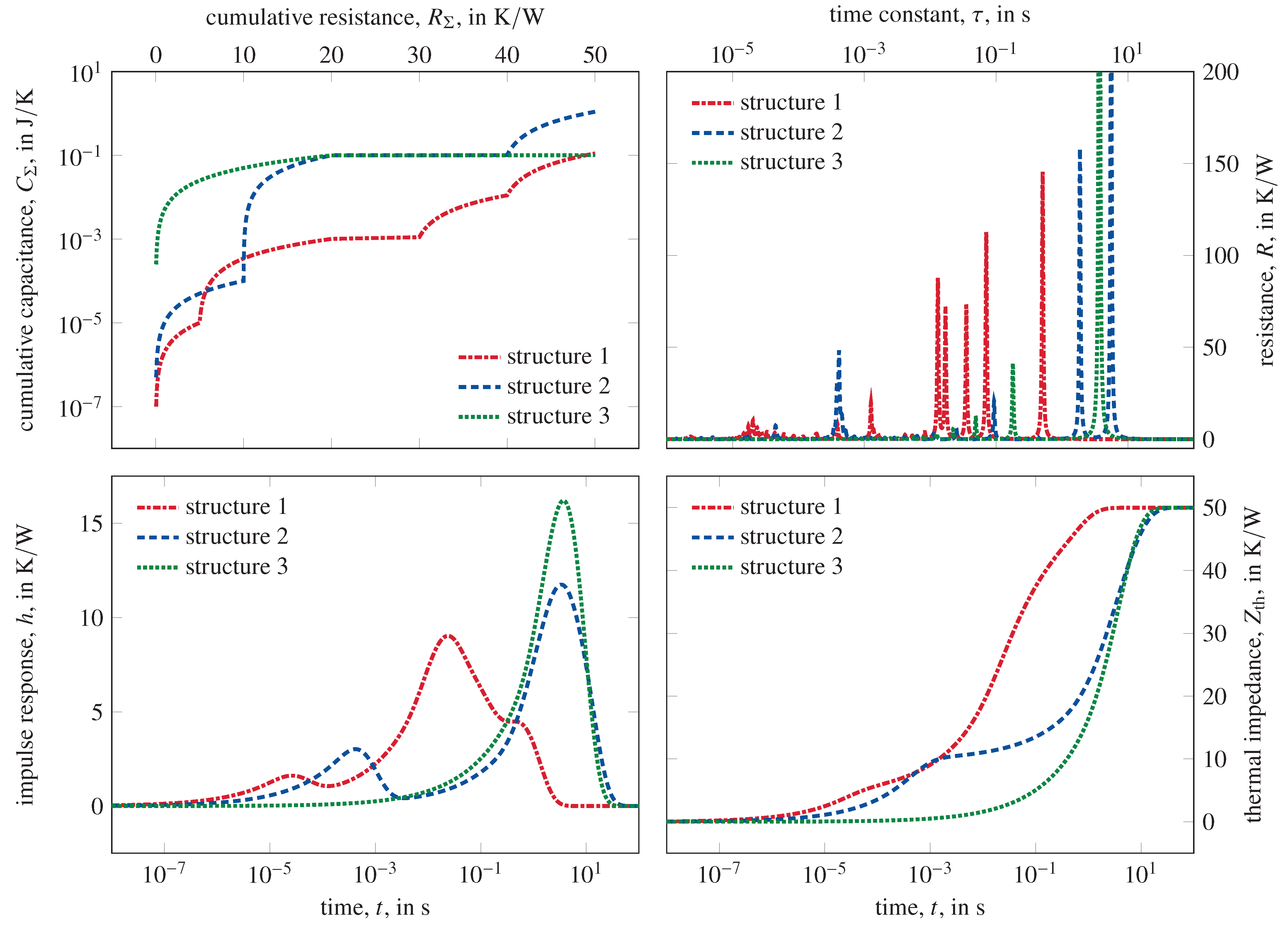
The thermal resistances, , and capacitances, , in Table 1 are chosen to be roughly similar to real electronic devices of varying complexity. While the time constant spectrum of structure 3 consists essentially of a single peak and has only three sections, structure 1 includes many smaller and larger peaks resulting from five sections. An illustration of the corresponding structure functions as well as the time constant spectra, impulse responses, and thermal impedances is given in Figure 3.
For realistic measurement data, the exact theoretical thermal impedance is covered by the addition of white noise. In this way, the performance of the algorithms is studied under non-ideal conditions. To avoid a systematic error, a high accuracy for the reference functions must be ensured. The first step is thus to investigate how large the error associated with the calculation of the theoretical thermal impedance is.
As the impedance, , of the piecewise uniform structure function has poles on the negative real axis, a small angle, , must be introduced. This, however, leads to a small systematic error in the calculation. While for smaller values of this kind of error decreases, at the same time the peaks in the time constant spectrum become narrower and consequently the discretization error increases. To compensate for this, the sampling rate of is increased. For all following calculations, is evaluated in the interval at a total of 1 × 10⁶ points. This increases the computation time of a theoretical thermal impedance to several minutes on the desktop computer used in this work (Windows 10, Intel Core i7-8665U CPU with GHz, 16 GB RAM).
All three test structures have a total thermal resistance of . Ideally, the theoretical thermal impedance should exactly match this value by satisfying the relation . However, due to the discretization error and the finite angle , is smaller than in practice. The difference is denoted as ,
Table 2 shows the values of averaged over the three test structures for different values of . As expected, the smallest value of shows the smallest deviation. To further reduce the error, a larger interval of is sampled to capture finer details at small values of . For all subsequent calculations, is chosen to be .
6. Performance Quantification
6.1. Parameter Comparison
For the calculations presented in this section, the input data consist of the exact thermal impedances belonging to thermal structure functions 1 to 3 and are comprised of 1 × 10⁶ uniformly distributed measurement points for . The solutions are compared to the theoretical ideal using the accuracy measures , , and as defined in (24), (25), and (27).
There are several parameters such as the window length increment, , and the number of points in the derivative, , which have to be specified as well. For some of these variables, tuning is crucial to guarantee a good performance. An obvious example is the cut-off frequency, , which determines the width of the filter during Fourier deconvolution. Other parameters, such as , have only a small effect on the result beyond a certain size. For a fair comparison between the methods, it is important to set these parameters to the identical values wherever possible.
Though Bayesian deconvolution also has a tunable parameter, namely the number of iterations, it is easier to handle than Fourier deconvolution. Figure 4 shows how the accuracy measure depends on the number of steps for Bayesian deconvolution. The number of steps tested covers three orders of magnitude from 1 × 10² to 5 × 10⁵. The accuracy converges with increasing number of steps, though the speed of convergence depends significantly on the complexity of the test structure. For structure 3, convergence for is not achieved even after 5 × 10⁵ steps.
The computation time for Bayesian deconvolution depends not only on the number of steps, but also on the number of data points, , as this determines the size of the matrices involved. For the calculations shown in Figure 4, the number of points was set to . Bayesian deconvolution with steps takes approximately half a minute. (Windows 10, Intel Core i7-8665U CPU with GHz, 16 GB RAM).
In all tested examples, convergence is achieved much later than discussed in the literature, which suggests the use of about 1000 steps [13,23]. However, according to the results depicted in Figure 4 it seems appropriate to use up to iteration steps and more.
Besides the process of deconvolution, derivation is also an important factor affecting the overall accuracy. In particular, this is true in the presence of noise. There are four important parameters in total which are varied when using optimal regression filtering. These are the minimum window length , the maximum window length , the window length increment , and the number of steps .
For all noise-free calculations, this includes the Bayesian deconvolution as well as Fourier deconvolution, the following configuration is used,
The window length, L, is measured in logarithmic time, z. This means a window of size corresponds to an interval of size in the thermal impedance. The starting window length is automatically chosen by the algorithm. In the presence of different levels of noise, the parameters have to be adjusted for optimum performance.
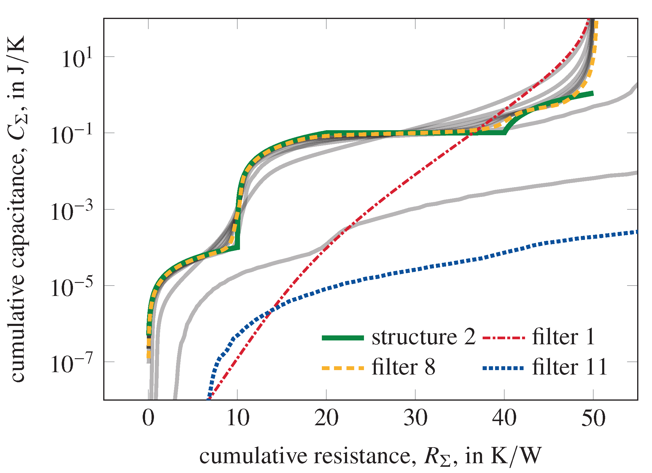
To illustrate the dependency of the result on the filter configuration, Figure 5 compares the ideal structure function for structure 2 with different solutions. Each solution is computed with the help of a Gaussian filter using different values of and fixed . Filter 1 is too narrow, leading to a significant loss of information in the result. In contrast, filter 11 is too wide, with the consequence that residual noise components are amplified and the total resistance is overestimated considerably. The best result is obtained for a filter width that lies in between Filter 1 and Filter 11. In the example, filter 8 performs best.
For Fermi and Gaussian filters, it is more difficult to find a good value for the filter configuration as these filters depend on two parameters. This is a significant disadvantage for Fermi and Gaussian filters, because the optimum filter has to be searched in a two-dimensional parameter space. In contrast, the Nuttall, Hann, and rectangular filters depend on one parameter only. To determine suitable filter configurations, a linear search as in Figure 5 is performed. This procedure must be repeated for each of the three test structures and both accuracy measures, and , all tested filters, namely the Fermi, Gaussian, Nuttall, Hann, and rectangular filters and different signal-to-noise ratios.
6.2. Performance in the Case of Perfect Data
Table 3 summarizes the performance metrics for all tested structures and methods without artificial noise added to the thermal impedance. A number of filter configurations is tested and the best one is selected in the sense explained above. This means, a different filter configuration is used to generate the accuracies for and . Results are summarized in Table 3. For Bayesian deconvolution, the number of points is set to and the number of steps is set to 5 × 10⁵.
A comparison of filter choices used in Fourier deconvolution shows mixed results with no clear winner which performs best on every metric. The rectangular filter shows good results for the time constant spectrum. The corresponding structure functions, however, are very inaccurate. The accuracy of the rectangular filter for the time constant spectrum vanishes in the presence of noise. The Hann filter stands out because it performs best among the Fourier based methods for on all structures. The additional effort of finding an optimum filter in a two-parameter space does not yield a more accurate result.
In practice, the use of for time constant spectra obtained via Fourier deconvolution tends to rank noise-induced oscillations in the spectrum better than one might intuitively expect. This is not the case for Bayesian deconvolution, where a strictly positive spectrum is guaranteed by the algorithm.
There is a clear trend in the computational difficulty of the three test structures. For almost all methods, the calculation of structure 1 gives the most accurate results. Nevertheless, the shape of its thermal structure function, time constant spectrum, and impulse response is complex (Figure 3 and Table 1). Structure 3 gives the least accurate results even though it includes only three sections. The Bayesian deconvolution performs best on this structure function, which has a sharply peaked time constant spectrum and profits greatly from the high amount of iteration steps used, see Figure 4.
6.3. Performance in Presence of Noise
Here, the amount of data forming the thermal impedance is reduced to 1000 points uniformly distributed on the -axis by interpolating the full size exact impedance. In addition, Gaussian noise with standard deviation defined via (28) is added to the theoretical thermal impedance. The tested signal-to-noise ratios are 50, 100, 200, 500, 1000, 2000, and 5000. As an example, for a transient thermal measurement with a total temperature rise of 100 and a measurement accuracy of 20 mK the signal-to-noise ratio amounts to .
For optimal performance, a tuning of the derivative parameters is very important. In all following calculations the setup (39) is used which achieves acceptable accuracy for all tested configurations,
Though individually adjusting the derivative parameters for every noise level would provide a slight gain in accuracy, here, a single set of derivative parameters is used. This is done to limit the number of free parameters and to reduce the influence of manually set parameters.
For Fourier deconvolution, it is not possible to use the same filter width for all signal-to-noise ratios. Instead, for every pair of window function and signal-to-noise ratio the parameters involved such as the cut-off frequency, , are manually tuned to achieve acceptable results. The manual tuning process of the filter parameters in the presence of noise is a tedious process. In contrast, for Bayesian deconvolution no adjustment is required, except for the number of iterations, which is set to 3 × 10⁴.
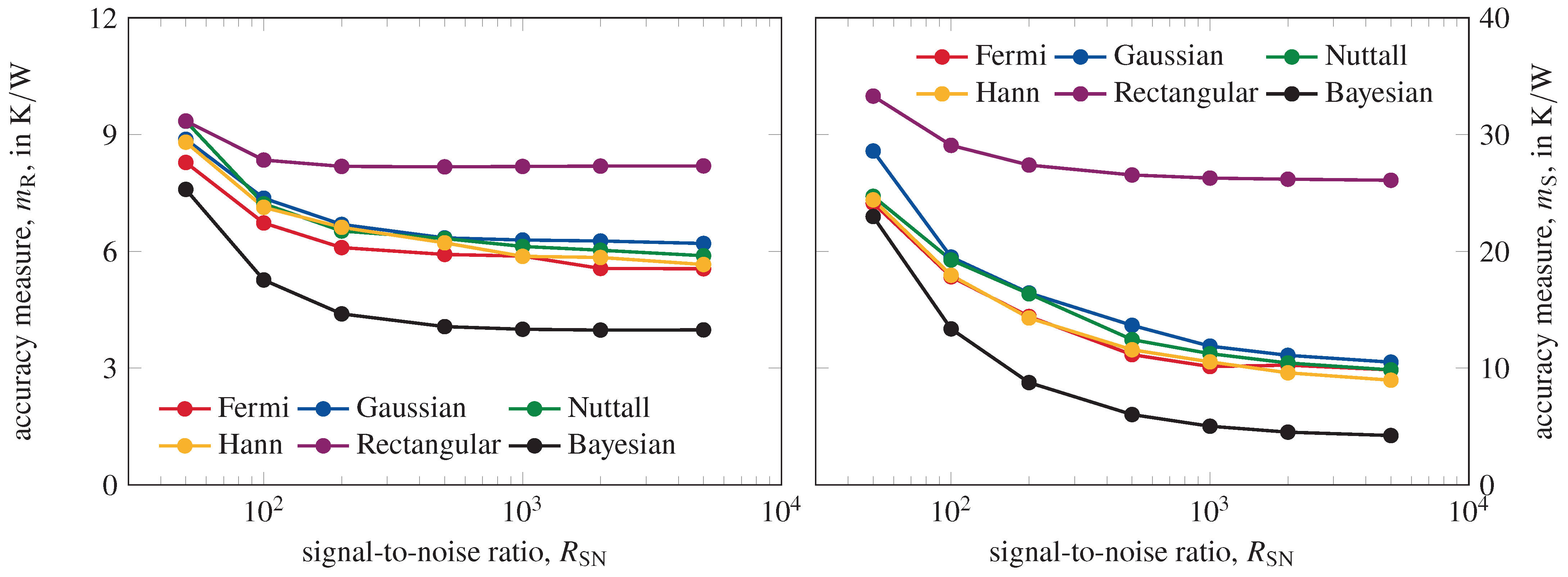
Figure 6 shows a comparison of the performance in the presence of noise for all window functions introduced above. The rectangular filter shows the worst performance on all metrics, while the Bayesian deconvolution retains its advantage even in the presence of noise. The relative difference between the methods decreases with increasing noise level. The Fermi and Hann window stand out as the more accurate filters. The Fermi window is the recommended filter according to [6]. However, the Hann window is easier to use in practice as it depends only on a single parameter while having comparable accuracy.
A comparison of the computational difficulties to recover structures 1 to 3 in the presence of varying noise level for Bayesian deconvolution is shown in Figure 7. Computations of structure 1 show the most accurate results while structure 3 appears the most difficult one to recover. The recovered structure function profits significantly more from a decreasing noise level than the time constant spectrum. Surprisingly, a good accuracy measure for the structure, , function is not necessarily based on a good .
7. Conclusions
Since its standardization by the JEDEC Solid State Technology Association, network identification by deconvolution has become a well-known measurement technique for determining thermal parameters in one-dimensional systems. Many implementations of the network identification algorithm exist. In this work, three measures of accuracy are presented to quantify the exactness of calculated time constant spectra and thermal structure functions. Using these measures, several variants of network identification by deconvolution are optimized and their performance is compared. To test the robustness of the algorithms, Gaussian noise of varying amplitude is added to the input data. Of all cases tested, Bayesian deconvolution with a large number of iteration steps, , has performed best. For Fourier deconvolution, the Hann window stands out as a good filter choice among the tested filters.
8. Patents
The technical content of the paper is related to a patent held by the authors under DE 10 2019 214 472.
Author Contributions
N.J.Z.: Conceptualization, methodology, software, investigation, writing—original draft preparation; P.W.N.: Conceptualization, validation, writing—review and editing; S.S.: Supervision, writing—review and editing. All authors have read and agreed to the published version of the manuscript.
Funding
This publication is funded by the Open Access Publication Fund of South Westphalia University of Applied Sciences.
Conflicts of Interest
The authors declare no conflict of interest.
References
- Codecasa, L.; Viti, F.D.; Race, S.; d’Alessandro, V.; Gualandris, D.; Morelli, A.; Villa, C.M. Thermal resistance and impedance calculator (TRIC). In Proceedings of the 25th International Workshop on Thermal Investigations of ICs and Systems (THERMINIC), Lecco, Italy, 25–27 September 2019; pp. 1–5. [Google Scholar] [CrossRef]
- Ezzahri, Y.; Shakouri, A. Application of network identification by deconvolution method to the thermal analysis of the pump-probe transient thermoreflectance signal. Rev. Sci. Instrum. 2009, 80, 074903. [Google Scholar] [CrossRef] [PubMed]
- Farkas, G.; Haque, S.; Wall, F.; Martin, P.S.; Poppe, A.; van Voorst Vader, Q.; Bognar, G. Electric and thermal transient effects in high power optical devices. In Proceedings of the Twentieth Annual IEEE Semiconductor Thermal Measurement and Management Symposium, San Jose, CA, USA, 11 March 2004; pp. 168–176. [Google Scholar] [CrossRef]
- Kim, H.H.; Choi, S.H.; Shin, S.H.; Lee, Y.K.; Choi, S.M.; Yi, S. Thermal transient characteristics of die attach in high power LED PKG. Microelectron. Reliab. 2008, 48, 445–454. [Google Scholar] [CrossRef]
- Székely, V.; Van Bien, T. Fine structure of heat flow path in semiconductor devices: A measurement and identification method. Solid-State Electron. 1988, 31, 1363–1368. [Google Scholar] [CrossRef]
- JC-15. Transient Dual Interface Test Method for the Measurement of the Thermal Resistance Junction to Case of Semiconductor Devices with Heat Flow trough a Single Path; Standard JESD51-14; JEDEC Solid State Technology Association: Arlington, TX, USA, 2010. [Google Scholar]
- Lasance, C.J.M.; Poppe, A. Thermal Management for LED Applications; Solid State Lighting Technology and Application Series; Springer: New York, NY, USA, 2016. [Google Scholar]
- Schweitzer, D.; Pape, H.; Chen, L. Transient measurement of the junction-to-case thermal resistance using structure functions: Chances and limits. In Proceedings of the Twenty-fourth Annual IEEE Semiconductor Thermal Measurement and Management Symposium, San Jose, CA, USA, 16–20 March 2008; pp. 191–197. [Google Scholar] [CrossRef]
- Schmid, M.; Bhogaraju, S.K.; Hanss, A.; Elger, G. A New Noise-Suppression Algorithm for Transient Thermal Analysis in Semiconductors Over Pulse Superposition. IEEE Trans. Instrum. Meas. 2021, 70, 1–9. [Google Scholar] [CrossRef]
- Salleras, M.; Palacin, J.; Carles, G.; Marco, S. Difficulties on the estimation of the thermal structure function from noisy thermal impedance transients. In Proceedings of the International Conference on Thermal and Mechanical Simulation and Experiments in Microelectronics and Micro-Systems, Como, Italy, 24–26 April 2006; pp. 1–7. [Google Scholar] [CrossRef]
- Szalai, A.; Székely, V. Possible acception criteria for structure functions. Microelectron. J. 2012, 43, 164–168. [Google Scholar] [CrossRef]
- Schmid, M.; Hanss, A.; Bhogaraju, S.K.; Elger, G. Time saving averaging algorithm for transient thermal analyses over deterministic pulse superposition. In Proceedings of the 25th International Workshop on Thermal Investigations of ICs and Systems (THERMINIC), Lecco, Italy, 25–27 September 2019. [Google Scholar] [CrossRef]
- Székely, V. Identification of RC networks by deconvolution: Chances and limits. IEEE Trans. Circuits Syst. Fundam. Theory Appl. 1998, 45, 244–258. [Google Scholar] [CrossRef]
- Pareek, K.A.; Grosse, C.; Sternberg, M.; May, D.; Ras, M.A.; Wunderle, B. Effect of Different Deconvolution Methods on Structure Function Calculation. In Proceedings of the 26th International Workshop on Thermal Investigations of ICs and Systems (THERMINIC), Berlin, Germany, 24 September 2020; pp. 97–104. [Google Scholar] [CrossRef]
- Prabhu, K. Window Functions and Their Applications in Signal Processing; CRC Press: Boca Raton, FL, USA, 2018. [Google Scholar]
- Székely, V. THERMODEL: A tool for compact dynamic thermal model generation. Microelectron. J. 1998, 29, 257–267. [Google Scholar] [CrossRef]
- Press, W.H.; Teukolsky, S.A.; Vetterling, W.T.; Flannery, B.P. Numerical Recipes 3rd Edition: The Art of Scientific Computing, 3rd ed.; Cambridge University Press: Cambridge, MA, USA, 2007. [Google Scholar]
- Szekely, V. Evaluation of short pulse thermal transient measurements. In Proceedings of the 14th International Workshop on Thermal Inveatigation of ICs and Systems, Rome, Italy, 24–26 September 2008; pp. 20–25. [Google Scholar] [CrossRef]
- Kennett, T.J.; Prestwich, W.V.; Robertson, A. Bayesian deconvolution I: Convergent properties. Nuclear Instrum. Methods 1978, 151, 285–292. [Google Scholar] [CrossRef]
- Kennett, T.J.; Prestwich, W.V.; Robertson, A. Bayesian deconvolution II: Noise properties. Nuclear Instrum. Methods 1978, 151, 293–301. [Google Scholar] [CrossRef]
- Kennett, T.J.; Brewster, P.M.; Prestwich, W.V.; Robertson, A. Bayesian deconvolution III: Applications and algorithm implementation. Nuclear Instrum. Methods 1978, 153, 125–135. [Google Scholar] [CrossRef]
- Ziegeler, N.J.; Nolte, P.W.; Schweizer, S. Thermal Equivalence Networks for Analysis of Transient Thermographic Data. In Proceedings of the 26th International Workshop on Thermal Investigations of ICs and Systems (THERMINIC), Berlin, Germany, 24 September 2020; pp. 226–231. [Google Scholar] [CrossRef]
- Székely, V. Enhancing reliability with thermal transient testing. Microelectron. Reliab. 2002, 42, 629–640. [Google Scholar] [CrossRef]
- Codecasa, L.; D’Amore, D.; Maffezzoni, P. Physical interpretation and numerical approximation of structure functions of components and packages. In Proceedings of the Semiconductor Thermal Measurement and Management IEEE Twenty First Annual IEEE Symposium, San Jose, CA, USA, 15–17 March 2005; pp. 146–153. [Google Scholar] [CrossRef]
- Gerstenmaier, Y.C.; Kiffe, W.; Wachutka, G. Combination of thermal subsystems modeled by rapid circuit transformation. In Proceedings of the 13th International Workshop on Thermal Investigation of ICs and Systems (THERMINIC), Budapest, Hungary, 17–19 September 2007; pp. 115–120. [Google Scholar] [CrossRef]
- Khatwani, K.J.; Bajwa, J.; Singh, H. Determining elements of lossy ladder networks. Electron. Lett. 1976, 12, 87–88. [Google Scholar] [CrossRef]
- Codecasa, L.; d’Alessandro, V.; Catalano, A.P.; Scognamillo, C.; D’Amore, D.; Aufinger, K. Accurate and efficient algorithm for computing structure functions from the spatial distribution of thermal properties in electronic devices. IEEE Trans. Electron Devices 2021, 1–8. [Google Scholar] [CrossRef]
- Codecasa, L.; Catalano, A.P.; d’Alessandro, V. A priori error bound for moment matching approximants of thermal models. IEEE Trans. Components Packag. Manuf. Technol. 2019, 9, 2383–2392. [Google Scholar] [CrossRef]
- Chen, W.K. Feedback, Nonlinear, and Distributed Circuits, The Circuits and Filters Handbook, 3rd ed.; CRC Press: Boca Raton, FL, USA, 2009. [Google Scholar]
- Krishnan, S.R.; Seelamantula, C.S. On the selection of optimum savitzky-golay filters. IEEE Trans. Signal Process. 2013, 61, 380–391. [Google Scholar] [CrossRef]
- Nuttall, A. Some windows with very good sidelobe behavior. IEEE Trans. Acoust. Speech Signal Process. 1981, 29, 84–91. [Google Scholar] [CrossRef] [Green Version]
Figure 1.
Foster-type RC-ladder network with n sections. Each section comprises a parallel resistance and capacitance.
Figure 1.
Foster-type RC-ladder network with n sections. Each section comprises a parallel resistance and capacitance.

Figure 2.
Cauer-type RC-ladder network with n sections. In this network, the resistances and capacitances correspond to the thermal equivalents in the device. As differentiation to the Foster network, Cauer-type components are denoted with a prime.
Figure 2.
Cauer-type RC-ladder network with n sections. In this network, the resistances and capacitances correspond to the thermal equivalents in the device. As differentiation to the Foster network, Cauer-type components are denoted with a prime.

Figure 3.
Overview on the three test structure functions (top left), their corresponding time constant spectra (top right), impulse responses (bottom left), and thermal impedances (bottom right), calculated at . For presentability, the time constant spectra plotted are calculated with .
Figure 3.
Overview on the three test structure functions (top left), their corresponding time constant spectra (top right), impulse responses (bottom left), and thermal impedances (bottom right), calculated at . For presentability, the time constant spectra plotted are calculated with .

Figure 4.
Accuracy of the time constant spectrum, , and structure function, , as a function of number of steps for Bayesian deconvolution. The number of points is set to .
Figure 4.
Accuracy of the time constant spectrum, , and structure function, , as a function of number of steps for Bayesian deconvolution. The number of points is set to .

Figure 5.
Various attempts (gray curves) for the cut-off frequency, , in a network identification using a Gaussian filter (35) for a fixed value of . Filter 1 is too narrow, filter 11 is too wide, while filter 8 yields the best result. For comparison, the ideal result for structure 2 is shown.
Figure 5.
Various attempts (gray curves) for the cut-off frequency, , in a network identification using a Gaussian filter (35) for a fixed value of . Filter 1 is too narrow, filter 11 is too wide, while filter 8 yields the best result. For comparison, the ideal result for structure 2 is shown.

Figure 6.
Accuracy of the median integrated time constant spectrum and median structure function, calculated via Fourier and Bayesian deconvolution as a function of the signal-to-noise ratio from 2000 noise realizations.
Figure 6.
Accuracy of the median integrated time constant spectrum and median structure function, calculated via Fourier and Bayesian deconvolution as a function of the signal-to-noise ratio from 2000 noise realizations.

Figure 7.
Accuracy of the median integrated time constant spectrum and median structure function calculated via Bayesian deconvolution for the three test structures as a function of the signal-to-noise ratio from 2000 noise realizations.
Figure 7.
Accuracy of the median integrated time constant spectrum and median structure function calculated via Bayesian deconvolution for the three test structures as a function of the signal-to-noise ratio from 2000 noise realizations.


Table 1.
Total thermal resistances and capacitances of the sections of the three piecewise uniform structure functions that serve as reference structures.
Table 1.
Total thermal resistances and capacitances of the sections of the three piecewise uniform structure functions that serve as reference structures.
| Structure 1 | Structure 2 | Structure 3 | ||||
|---|---|---|---|---|---|---|
| Sections | K/W | J/K | K/W | J/K | K/W | J/K |
| Section 1 | 5 | 1 × 10 | 10 | 1 × 10 | 20 | 1 × 10 |
| Section 2 | 15 | 1 × 10 | 10 | 1 × 10 | 20 | 1 × 10 |
| Section 3 | 10 | 1 × 10 | 10 | 1 × 10 | 10 | 1 × 10 |
| Section 4 | 10 | 1 × 10 | 10 | 1 × 10 | - | - |
| Section 5 | 10 | 1 × 10 | 10 | 1 × 10 | - | - |
Table 2.
Deviation in thermal impedance averaged for structure 1 to 3 at various .
| 5.00 | 3.50 | 2.00 | 1.50 | 0.50 | 0.10 | 0.03 | |
| 2.82% | 1.98% | 1.15% | 0.87% | 0.32% | 0.09% | 0.05% |
Table 3.
Best accuracy for all methods in the absence of noise. The best performing method in each column is double underlined, the second best result is underlined. The first five methods denote selections for the window functions, .
Table 3.
Best accuracy for all methods in the absence of noise. The best performing method in each column is double underlined, the second best result is underlined. The first five methods denote selections for the window functions, .
| Structure 1 | Structure 2 | Structure 3 | |||||||
|---|---|---|---|---|---|---|---|---|---|
| Method | K/W | K/W | K/W | K/W | K/W | K/W | K/W | K/W | K/W |
| Fermi | 4.7 | 7.7 | 0.06 | 5.8 | 9.6 | 0.91 | 8.1 | 16.3 | 2.91 |
| Gaussian | 5.1 | 8.9 | 0.08 | 7.6 | 09.4 | 0.27 | 9.3 | 13.8 | 0.09 |
| Nuttall | 4.7 | 8.2 | 0.12 | 6.8 | 8.5 | 0.38 | 10.1 | 11.5 | 0.15 |
| Hann | 4.4 | 7.4 | 0.28 | 6.3 | 7.5 | 0.44 | 8.9 | 10.8 | 0.91 |
| Rectangular | 4.0 | 38.7 | 6.94 | 5.4 | 41.4 | 6.31 | 7.6 | 129 | 31.08 |
| Bayesian | 3.4 | 3.7 | 0.04 | 3.8 | 4.4 | 0.02 | 5.7 | 3.1 | 0.01 |
Publisher’s Note: MDPI stays neutral with regard to jurisdictional claims in published maps and institutional affiliations. |
© 2021 by the authors. Licensee MDPI, Basel, Switzerland. This article is an open access article distributed under the terms and conditions of the Creative Commons Attribution (CC BY) license (https://creativecommons.org/licenses/by/4.0/).
Share and Cite
MDPI and ACS Style
Ziegeler, N.J.; Nolte, P.W.; Schweizer, S. Quantitative Performance Comparison of Thermal Structure Function Computations. Energies 2021, 14, 7068. https://0-doi-org.brum.beds.ac.uk/10.3390/en14217068
AMA Style
Ziegeler NJ, Nolte PW, Schweizer S. Quantitative Performance Comparison of Thermal Structure Function Computations. Energies. 2021; 14(21):7068. https://0-doi-org.brum.beds.ac.uk/10.3390/en14217068
Chicago/Turabian StyleZiegeler, Nils J., Peter W. Nolte, and Stefan Schweizer. 2021. "Quantitative Performance Comparison of Thermal Structure Function Computations" Energies 14, no. 21: 7068. https://0-doi-org.brum.beds.ac.uk/10.3390/en14217068
Note that from the first issue of 2016, this journal uses article numbers instead of page numbers. See further details here.