Does Air Pollution Impact Fiscal Sustainability? Evidence from Chinese Cities

Abstract

Fiscal sustainability is an issue of great concern for governments globally and air pollution control has become an important factor affecting fiscal sustainability. This study aims to examine the impact of air pollution on fiscal sustainability in the short and long run. We conducted an empirical analysis based on air pollution and local government debt data on China’s prefecture-level cities in 2014–2019, using regression discontinuity design (RDD) and a panel data model. The results show that air pollution reduces the debt burden of governments in the short run. However, in the long run, addressing the negative impacts of air pollution adds to the debt burden of local governments, hindering fiscal sustainability. Fiscal freedom and the level of public services significantly moderate the negative impact of air pollution on fiscal sustainability. A higher level of fiscal freedom generally indicates a greater incentive for local governments to raise pollutant emission standards, strengthen the construction of green infrastructure, and subsidize green enterprises. Furthermore, a higher level of public services reflects better infrastructure and higher levels of investment in environmental protection, which help to reduce the negative impact of air pollution. The governments are suggested to take measures to effectively control air pollution, so as to enhance fiscal stability in the long run.

1. Introduction

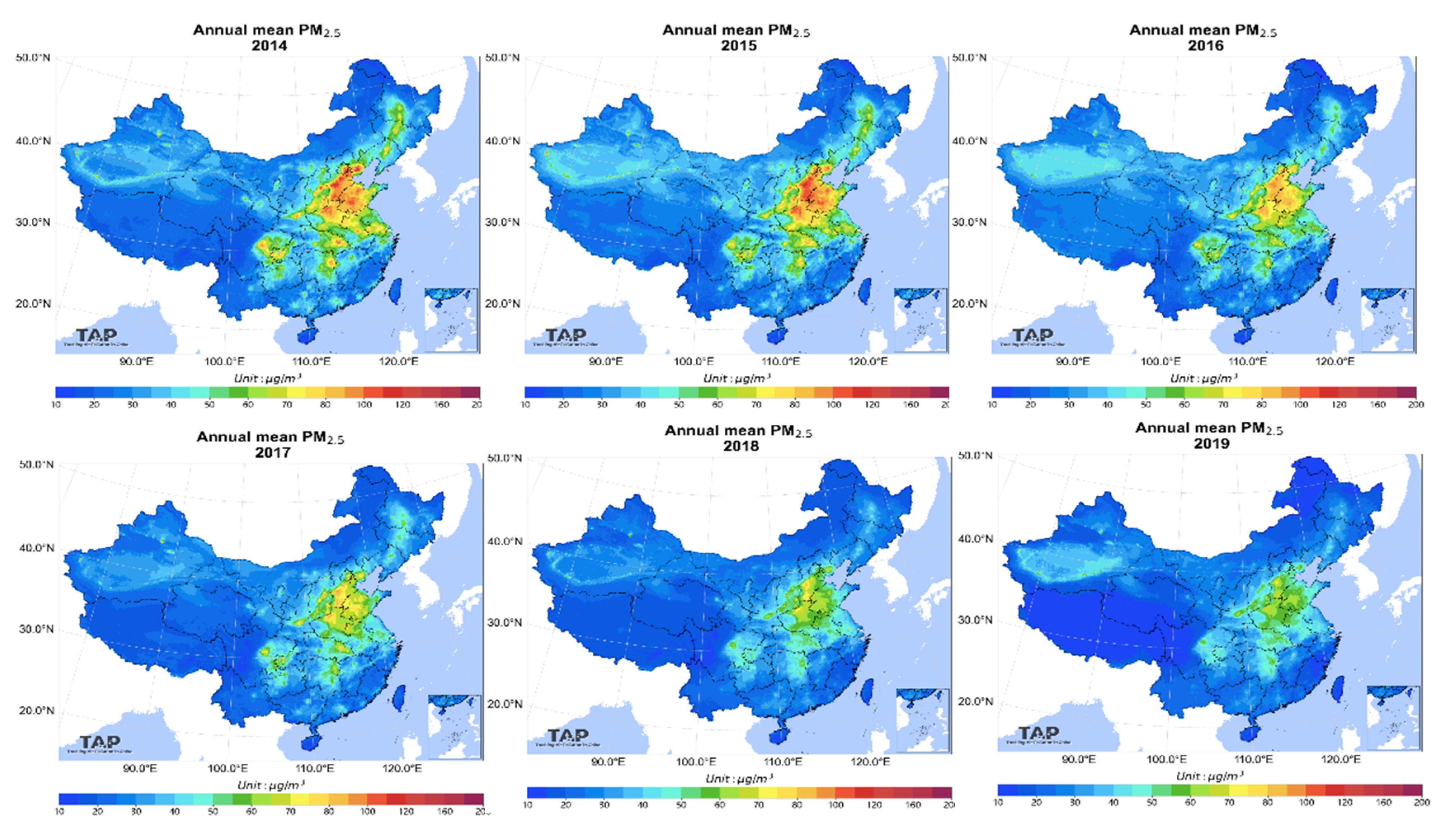
Environmental problems, such as air pollution, are issues of global concern. As the world’s largest developing country, China has attached great importance to managing the prevention and control of atmospheric pollution. Since the 18th National Congress of the Chinese Communist Party in 2012, the Chinese government has made the “Blue Sky Protection Campaign” a top priority in the uphill battle for the prevention and control of pollution and has declared a war on pollution with unprecedented determination and strength. After years of hard work, China has begun to reap the fruits of such efforts. Overall air quality has improved, and significant improvements have been seen in key areas. However, air pollution remains a serious problem and there remain major challenges in controlling it. According to historical data, the PM25 concentration in China shows a downward trend (Figure 1 and Figure 2) [1,2,3], but there is still a long way to go before it falls below the World Health Organization’s standard of 10 micrograms per cubic meter. Deteriorating weather conditions will also lead to increased air pollution (Figure 3) [1,2,3].

Fiscal policy plays an important role in air pollution control. For example, the government can directly control air pollution through direct investment or transfer payments; the government can also indirectly affect corporate behavior through procurement and tax incentives to achieve air pollution prevention. Such policy measures inevitably cause governments financial pressures in the short run; thus, air pollution control has become an important factor affecting public finance sustainability.

Fiscal sustainability is a key aspect of the organization and management of local governments globally [4,5]. Various scholars have defined fiscal sustainability. For instance, in [6], the authors point out that, on the one hand, fiscal sustainability refers to solvency (i.e., a government’s ability to repay debts without explicit default) and, on the other hand, it refers to a government’s ability to maintain its current set of policies while also maintaining solvency. The International Public Sector Accounting Standards Board regards fiscal sustainability as the ability of an entity to fulfill its service obligations and financial commitments now and in the future. In [7], the authors define fiscal sustainability as a situation in which a government can provide services now and in the future without this being destructive to revenue or its ability to spend. In [8], the authors describe the three main prerequisites for ensuring the fiscal sustainability of the public sector: (a) deficits should be a temporary phenomenon balancing out the economic cycle, (b) debt should remain stable over the economic cycle, and (c) debt should be secured by assets of at least the same value.

Based on the existing studies, it is evident that debt is an important aspect of evaluations of fiscal sustainability. Therefore, we use debt as a proxy for fiscal sustainability in our research. In addition, if local fiscal management focuses on fiscal sustainability, it may conflict with fiscal management oriented toward improving public services [5]. In other words, the key to fiscal sustainability is not to minimize spending, but instead to raise reasonable levels of debt to drive local economic growth effectively and provide the best level of public services.

Regarding the debt indicators used to measure fiscal sustainability, the International City Management Association points out that the debt burden of local governments is an important indicator of the fiscal sustainability of governments and is usually measured using the ratio of government debt divided either by the population or GDP [9]. In our research, the sustainability of local finances is an important factor in evaluating the financial status of local governments, that is, allowing the government to continue to provide services and fulfill its obligations. The sustainability of local finances is fluid and dynamic across the time dimension because it is not only related to the government’s ability to meet current service needs, but also to the government’s ability to meet future service needs. Based on this, the ratio of local government debt to GDP is chosen to measure the fiscal sustainability of local governments in this study, and the ratio of local government debt to population is used as a replacement variable for robustness testing.

Existing studies focus on the relationship between air pollution prevention and individuals at the micro level. For instance, in [10], the authors focused their study on the impact of air quality on enterprises and residents. They applied the Ambient Air Quality Standards, as revised in 2012, to a quasi-natural experiment. The results of RDD show that the implementation of the new air quality standards had several benefits. For enterprises, they created a positive policy environment for green enterprises and suggested new requirements for the optimization of corporate management and the ability of CEOs to lead their companies efficiently. For residents, they promoted desire amongst members of the community to protect the environment. In [11], the authors found that the more serious the air pollution is in the cities where the headquarters of listed companies are located, the lower the quality of the human capital of the company’s management. Scholars have also pointed out that air quality affects people’s physical and mental health by inducing health issues such as respiratory infections, cerebrovascular diseases, and cardiopulmonary infections [12,13,14,15].

At the macro level, air pollution also affects national economic growth and social development. Improvements in environmental quality lead to higher quality of life, but may raise the challenge of limiting economic growth and increasing urbanization rates [16]. Green infrastructure can bring environmental, social, and economic benefits [17,18,19], such as reducing the urban heat island effect, increasing carbon dioxide storage, improving water and air quality, increasing social cohesion, raising entertainment and tourism opportunities, and lifting the value of real estate [20].

In view of the current situation, it is crucial for China to promote green economic development, build an ecological civilization, promote a new paradigm of economic development, and improve the fiscal sustainability to achieve green development.

However, few studies have analyzed the economic effects of air pollution prevention and control from the perspective of fiscal sustainability, especially with regards to the level of local government debt. This study empirically tests the relationship between air pollution prevention and fiscal sustainability based on data from China’s prefecture-level cities in 2014–2019.

This study contributes to the existing literature in two ways. First, this research distinguishes the long-run and short-run effects of air pollution on fiscal sustainability and explores the moderating effects of factors such as fiscal freedom and public service level. Second, it provides new research perspectives on sustainable fiscal development to understand the economic effects of air pollution prevention and control.

2. Literature Review and Hypothesis Development

2.1. Short-Run Impact of Air Pollution on Fiscal Sustainability

Due to “yardstick competition”, local governments are motivated to pursue economic development as they compete to earn political achievements [21]. Research shows that yardstick competition between local governments centering on comparing political performance is a common practice in China [22]. As economic growth indicators account for a large proportion of the evaluation of political performance, local governments have strong incentives to participate in so-called “GDP championships” [23]. In a system in which political power is centralized and fiscal power is decentralized, to earn political promotions, local government officials work to integrate the economic and political resources under their control to promote rapid regional economic growth.

Many city governments have chosen to focus on driving economic growth at the expense of the environment, at least in the short term. In China’s five-level administrative structure, government is divided into central, provincial, municipal, county, and township levels. The power of the central government to supervise levels below it grows weaker further down the government hierarchy due to information asymmetry. Owing to self-interested motives, local officials also seek to maximize their own personal power, prestige, security, and income (i.e., they aim to maximize their personal interests rather than public interests) [24] and display opportunistic behaviors that can be contrary to the will of the central government and maximization of public interest.

Therefore, it is reasonable to believe that local governments are motivated to pursue economic growth in the short run rather than engage in borrowing for green investment. As a result of the simultaneous deterioration of air quality, rapid economic growth, and strengthening of fiscal affordability, air pollution may be negatively correlated with the debt burden of local finance. Thus, the following hypothesis is proposed:

Hypothesis 1 (H1).

In the short run, air pollution has a positive correlation with fiscal sustainability.

2.2. Long-Run Impact of Air Pollution on Fiscal Sustainability

Studies have shown that the stability and balance of government debt are important premises to ensure fiscal sustainability, and also important supports for the government to provide sustainable public services [14,23].

Hangover effect. When the accumulation of air pollution reaches a certain level, local governments must take measures to raise debt to fund improvements to the environment. The cumulative deterioration of air quality promotes the increasing participation of public capital and other forms of social capital in environmental governance, forcing the government to carry out environmental governance and institutional reform. For example, in [25], the authors stated that when residents have the right to migrate freely, they “vote with their feet” and migrate to areas that offer public services consistent with their preferences. Not only does this solve the signaling problem of public services, but it also places pressure on local governments to improve public services. In [26], the authors conducted an empirical analysis of 85 local cities and towns in China, finding that the government’s preference for environmental pollution control is affected by the complaints of residents in the region. In other words, the complaints of residents regarding air quality affect the degree to which local governments put resources into managing air pollution. In [27], the authors estimated the value of clean air using the sales of air purifiers and anti-smog masks as an indicator. Their study shows that people are willing to pay for clear air, as sales of these goods increased as air quality deteriorated. In the long run, the air pollution caused by blindly pursuing economic development without the appropriate policies and mitigations in place can lead to strong demand from the public which in turn results in strict supervision by local governments. In order to save money in the long run, local governments must close loopholes in environmental protection laws, improve green infrastructure, and increase investment in environmental governance by borrowing. Such investments include strengthening the construction of green infrastructure [28], subsidizing green enterprises, developing more energy efficient vehicles and low-carbon fuels, and improving urban planning to facilitate green public transportation. In the short run, however, this would require increasing the debt burden of local governments.

Collateral effect. Air pollution can affect people’s physical and mental health, increase the tendency of residents to migrate, and cause housing prices to fall [29]. As income and education increase nationally, people have become more aware of the harm caused by air pollution, and this increased awareness has led to labor migration, especially amongst high-level innovative talent [30]. In [31], the authors found that air pollution affects people’s willingness to migrate. When air pollution is high, internet searches for “migration” increase. For each 100-point increase in the air quality index (AQI), the search frequency of “migrants” increases by 2.3–4.8%. As residents’ tendency toward migration increases due to worsening air pollution, urban housing prices decrease [32,33]. There is a significant “collateral effect” in a prosperous real estate market. When housing prices rise, the price of government-owned houses and the income from land sales will increase, and the external debt repayment capacity of local governments can be improved. However, the contraction of the real estate market caused by air pollution is not conducive to the government’s debt repayment. The main sources of local governments’ debt financing are short- and medium-term loans from financial institutions, but these funds are mostly invested in long-term infrastructure projects [34,35]. This maturity mismatch leads to a high dependence on incomes obtained or collected from land and real estate, including land transfer fees and land- and real estate-related taxes and fees [36]. Thus, we propose the following hypothesis:

Hypothesis 2 (H2).

In the long run, air pollution aggravates the debt burden of local governments, which is not conducive to fiscal sustainability.

Based on the above analysis, the impact mechanism of air pollution on fiscal sustainability is illustrated in Figure 4.

3. Data, Variables, and Model

3.1. Data

In this study, the debt data of local governments were retrieved from the iFinD database, and the air pollution data came from the China Environment Yearbook, the Data Center of the Ministry of Ecology and the Environment of China, and the ERA-Interim database. The urban-level macroeconomic data came from the China City Statistical Yearbook, China Statistical Yearbook for the Regional Economy, China Land and Resources Statistical Yearbook, Finance Yearbook of China, iFinD database, and ERA-Interim database. Data on municipalities and observations that lack key variables were omitted and 236 cities remained.

3.2. Variables

3.2.1. Air Pollution (PM25)

The PM25 emission concentrations of China’s prefecture-level cities were used as the core air pollution indicator because the sample selected in this study covers a long period. By contrast, data on other pollutants are difficult to obtain or have continuous spans that are shorter, which makes them unsuitable for panel analysis, and there may also be problems such as data fraud and manipulation. The PM25 data, which were retrieved from satellite maps and are jointly released by Columbia University and the United States Atmospheric Composition Group, are objective and provide wide coverage. In addition, in the robustness tests, we follow [37,38] by introducing PM10 and the AQI as proxy indicators of air pollution to more comprehensively examine the impact of air pollution on fiscal sustainability. These data were retrieved from the Data Center of the Ministry of Ecology and the Environment of China and China Environment Yearbook.

To solve the endogeneity problem of environmental regulations, following [39], the coefficient of air flow was taken as the instrumental variable of air pollution. According to [40], the coefficient of air flow is the product of the wind speed and height of the boundary layer. The ERA-Interim database of the European Centre for Medium-Range Weather Forecasts provides data at 10 m altitude on wind speeds and boundary layer altitudes in a 0.75° × 0.75° global grid (approximately 83 square kilometers). In this study, the coefficient of air flow of each grid in the corresponding years were first calculated before matching the grids with the cities in the sample according to latitude and longitude. The coefficient of air flow of the cities in each year were then obtained.

3.2.2. Fiscal Sustainability (debtgdp)

In our research, local fiscal sustainability is an important factor for evaluating the financial situation of local governments. Fiscal stability allows local governments to provide services and fulfill their ongoing obligations. In other words, fiscal stability relates to the ability of the government to satisfy current and future demands for services. Based on this, the leverage ratio of the local government (the ratio of the local government’s debt to GDP) was selected to measure its fiscal sustainability. In the robustness test, we followed [5,7] by using local government debt/population and local government debt/resident income to measure fiscal sustainability.

3.2.3. Moderating Variables

The fiscal freedom and the public service capability were selected as moderating variables based on the literature review. The fiscal freedom is measured by the ratio of local budgeted revenue to local budgeted expenditure. Regional per capita fiscal expenditure was used as the proxy of the regional public service level.

3.2.4. Control Variables

Following previous literature [41,42,43], we chose a set of variables that reflect the characteristics of urban economics and public goods, including the GDP growth rate, population growth rate, urbanization rate measured by the proportion of non-agricultural employment to total employment, the ratio of the secondary industry added value to GDP represented the industrial structure, the ratio of financial institutions’ loan balances to GDP represented financial resources, and the ratio of fixed asset investment to GDP represented dependence on investment. The unemployment rate and healthcare conditions measured by the number of hospital beds per capita were also used to control for the impact on fiscal sustainability.

Table 1. Variable definitions.

Indicator	Variable	Definition	Mean	Min	Max
Air pollution	PM25	The average concentration of PM25 emissions in each region	67.86	9	276
	PM10	The average concentration of PM10 emissions in each region	106.73	18	382
	AQI	Air quality index in each region	97.02	18	301
Fiscal sustainability	debtgdp	Local government leverage ratio, local government debt divided by GDP	14.94	0.47	49
Cutoff (driving variable)	north	Latitude of the city: 33rd parallel north, the north/south boundary	−0.87	−14.64	17.50
Moderating variables	fsr	Fiscal freedom, measured by the ratio of local budgeted revenue to local budgeted expenditure	0.46	0.11	1.99
	ps	Regional public service level, with regional per capita fiscal expenditure as the proxy variable	6435.68	1.99	44,938.86
Control variables	pg	Population growth rate	6.40	−16.67	40.60
	dgdp	GDP growth rate	7.35	−31.1	109.10
	sgdp	Industrial structure, measured by the ratio of secondary industry added value to GDP	45.67	12.38	80.07
	fin1	Financial resources, measured by the ratio of financial institutions’ loan balance to GDP	0.98	0.22	14.18
	fa	Dependence of GDP on investment, measured by the ratio of fixed asset investment to GDP	0.82	0.17	2558
	ur	Unemployment rate, measured by annual registered unemployment rate in urban areas	3.12	1.12	4.90
	urban	Urbanization rate, measured by the proportion of non-agricultural employment to total employment	0.63	0.25	0.99
	bed	Healthcare conditions, measured by the number of hospital beds per capita	0.45	2.97 × 10−7	0.98

presents the variable definitions and descriptive analysis.

Table 2. Pairwise correlations.

Variables	(1)	(2)	(3)	(4)	(5)	(6)	(7)	(8)	(9)	(10)	(11)	(12)
(1) PM25	1.000
(2) debtgdp	−0.118 ***	1.000
(3) dgdp	0.049 *	−0.016	1.000
(4) sgdp	0.106 ***	−0.072 **	0.124 ***	1.000
(5) pg	0.001	−0.055 *	0.102 ***	−0.001	1.000
(6) fin1	−0.120 ***	0.194 ***	−0.063 **	−0.405 ***	−0.072 **	1.000
(7) fa	0.187 ***	−0.101 ***	0.179 ***	0.030	−0.016	−0.201 ***	1.000
(8) ur	0.109 ***	0.015	−0.045	0.060 **	−0.204 ***	−0.104 ***	0.155 ***	1.000
(9) urban	0.097 ***	0.039	−0.001	0.227 ***	−0.124 ***	0.213 ***	−0.222 ***	−0.156 ***	1.000
(10) fsr	0.081 ***	0.045	0.090 ***	0.225 ***	0.048	0.197 ***	−0.247 ***	−0.317 ***	0.680 ***	1.000
(11) ps	−0.102 ***	0.019	−0.044	−0.077 ***	−0.066 **	0.117 ***	−0.008	−0.003	0.081 ***	0.058 **	1.000
(12) bed	0.006	0.092 ***	−0.038	−0.007	0.133 ***	−0.272 ***	0.165 ***	0.245 ***	−0.363 ***	−0.362 ***	−0.036	1.000

*** p < 0.01, ** p < 0.05, * p < 0.1.

reports the results of correlation analysis. As shown in Table 2, PM25 negatively influences debtgdp. Because most of the variables are ratios or proportions, the pairwise correlations are low, similar to relevant literature [39].

3.3. Model

A panel data model with city fixed effects was constructed to investigate how air pollution impacts fiscal sustainability, according to the results of Hausman tests. Given that government debt usually matures after three to five years, local governments would have large financing demands due to the greater scales and pressures of repayment. In particular, more than 50% of the new debt borrowed in the fifth year is used to repay the maturing stock debt [44], showing that governments’ debt repayment pressures are concentrated mainly in the fifth year. Therefore, to study the long-run impact of air pollution on fiscal sustainability, the air pollution degree was lagged by five periods while the other control variables were only lagged by one period. For this reason, the following settings were adopted in the benchmark regression:

$$Debtgd{p}_{i,t}=\alpha +\beta \ast PM{25}_{i,t}+X_{i,t}\ast \gamma +{\theta }_i+{\epsilon }_{it}$$

(1)

$$Debtgd{p}_{i,t}=\alpha +\beta \ast PM25\_5_{i,t}+X\_1_{i,t}\ast \gamma +{\theta }_i+{\epsilon }_{it}$$

(2)

where $Debtgd{p}_{i,t}$ denotes the local government leverage ratio, $PM{25}_{i,t}$ denotes the air pollution degree, $PM25\_5_{i,t}$ denotes the air pollution degree lagged by five periods, $X_{i,t}$ denotes the control variables, and $X\_1_{i,t}$ denotes the control variables lagged by one period. The model also includes the city fixed effect ${\theta }_i$ and stochastic error term ${\epsilon }_{it}$.

4. Empirical Results

4.1. Regression Discontinuity Design

Graphical analysis of an RDD can vividly show the conditional density jump of the explained variable at the breakpoint, and the analysis is more random [45]. Given that the average temperature in northern China is much lower than that in the south, since the beginning of the planned economy era in 1949, the Chinese central government has implemented different policies for indoor heating during the winter for northern and southern regions. In most northern cities, the government subsidizes the use of coal for indoor heating in winter; this is called the Huai River Policy. As the use of coal causes high levels of pollutants to be emitted, other conditions being equal, the air quality in northern cities is worse than that in southern cities. This phenomenon has been confirmed in the literature. For example, in [46], the authors point out the considerable leap in air pollution from the south of the Huai River to the north of the Qin Mountains.

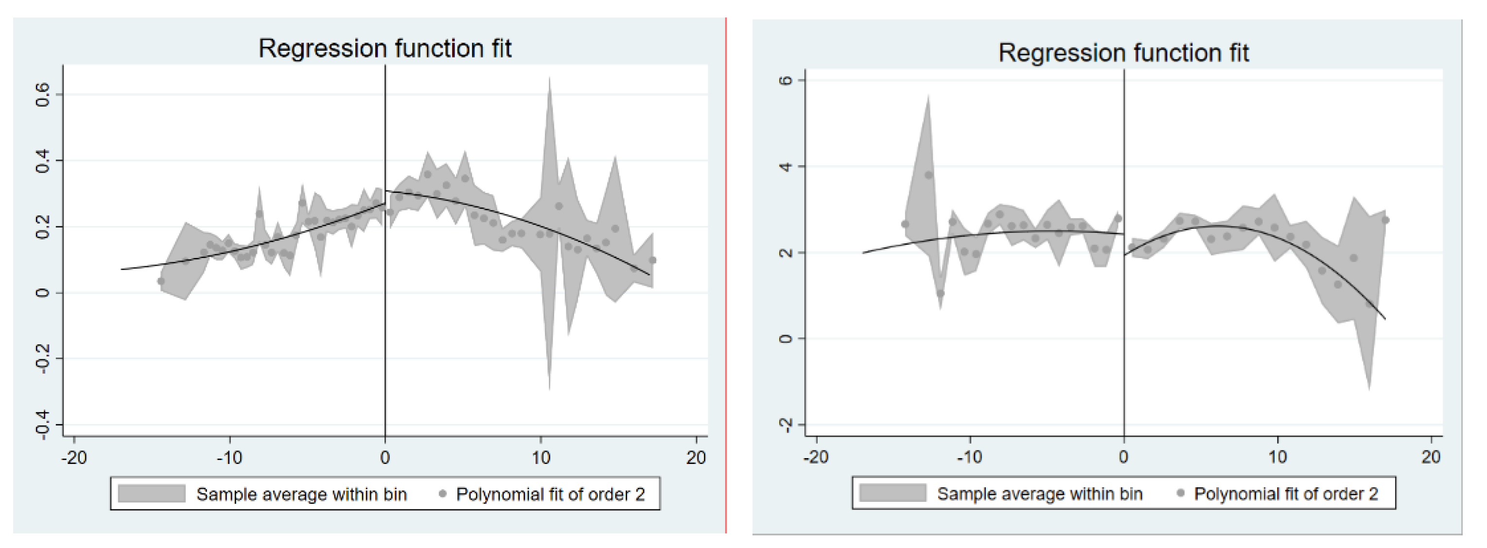
Therefore, this study refers to the quasi-natural experiment conducted by [47], which was generated by China’s centralized winter heating policy implemented in the north of the Qin Mountains-Huai River boundary (Qin-Huai boundary) and the RDD method is used to estimate the impact of air pollution on fiscal sustainability. The RDD graph is composed of two variables: the local government leverage ratio (debtgdp) and air pollution (PM25) (Figure 5). The horizontal axis represents the difference (north) between the location dimension of a city with a symmetrical bandwidth of 15° and 33° north latitude while the vertical axis represents the average values of the local government leverage ratio (debtgdp) and air pollution (PM25). Owing to the centralized heating policy in northern China, there is a significant cutoff of air pollution on the Qin-Huai boundary. Air pollution in southern China is lower than in the north (left side of the figure) and the fiscal sustainability of the south is lower than in the north (right side of the figure). These preliminarily data support Hypothesis 1 and provide an opportunity to further identify the impact of air pollution on the ability of local governments to pursue sustainable fiscal development.

Another condition should also be satisfied before the use of the RDD method: the non-manipulability test of the driving variable. Indeed, a key assumption in an RDD is that an individual cannot accurately manipulate the driving variables. The method of [48] is adopted to test whether the density distribution function of the driving variable (the latitude difference between the geographic location of a prefecture-level city and Qin-Huai boundary) is continuous. The abscissa in Figure 6 represents the latitude difference between the geographical location of the prefecture-level city and the Qin-Huai boundary. The dots in the figure represent the density distribution and the solid line represents the fitted values of the driving variable’s density function at a 95% confidence interval. The density distribution is smooth and continuous on the Qin-Huai boundary while the estimated discontinuity of the density function is −0.023 and the standard deviation is 0.142. This does not reject the null hypothesis that the density distribution of prefecture-level cities is smooth and continuous at the boundary. Therefore, there is no evidence that the government has manipulated the location of prefecture-level cities. As the dividing line of the centralized winter heating policy, the Qin-Huai boundary is determined by its geographical temperature in January of 0 °C. The formation of the boundary does not serve any other political or economic purpose, and it thus meets the requirements of the randomness assumption.

4.2. Ordinary Least Squares Estimation

4.2.1. Main Conclusion

Table 3. Air pollution and fiscal sustainability.

.	(1)	(2)	(3)	(4)	(5)	(6)	(7)	(8)
VARIABLES	debtgdp	debtgdp	debtgdp	debtgdp	debtgdp	debtgdp	debtgdp	debtgdp
PM25	−0.012 ***	−0.009 **
	(0.004)	(0.004)
PM10			−0.017 ***	−0.009 ***
			(0.003)	(0.003)
PM25_5					0.006 **	0.006 **
					(0.003)	(0.003)
PM10_5							0.004 **	0.005 **
							(0.002)	(0.002)
dgdp		−0.659 **		−0.645 **
		(0.282)		(0.282)
sgdp		−8.674 ***		−8.389 ***
		(1.004)		(1.013)
pg		−0.082		−0.060
		(0.156)		(0.156)
fin1		2.946 ***		2.693 ***
		(0.918)		(0.921)
fa		−1.992 **		−2.172 **
		(0.973)		(0.972)
ur		−1.316		−1.274
		(1.336)		(1.332)
urban		8.566 **		8.614 **
		(4.093)		(4.083)
bed		0.118		0.110
		(0.126)		(0.126)
Control_1						YES		YES
Constant	−17.549 ***	−17.073 ***	−16.571 ***	−16.786 ***	−18.378 ***	−18.632 ***	−18.381 ***	−18.635 ***
	(0.268)	(0.286)	(0.295)	(0.324)	(0.081)	(0.096)	(0.081)	(0.096)
Observations	1281	1032	1281	1032	1276	1022	1276	1022
R-squared	0.936	0.947	0.938	0.947	0.934	0.930	0.934	0.930
Adj R-squared	0.922	0.933	0.924	0.933	0.919	0.908	0.919	0.908
F	9.55	20.16	38.80	20.61	5.00	1.85	4.73	1.93
Within R-sq.	0.009	0.183	0.036	0.186	0.005	0.019	0.005	0.019
Root MSE	2.872	2.614	2.832	2.608	2.908	3.039	2.908	3.037
CITY FE	YES	YES	YES	YES	YES	YES	YES	YES

Standard errors in parentheses. *** p < 0.01, ** p < 0.05.

presents the benchmark results of the impact of air pollution on fiscal sustainability. No control variables are added in Columns (1) and (5). The results show that in the short run, for every 1% increase in PM25, the debt burden drops by 1.2%. In the long run, for every 1% increase in PM25, the debt burden increases by 0.6%. The regression coefficients are significantly positive at the 5% and 1% confidence intervals, respectively. The control variables are added into Columns (2) and (6).

The results show that in the short run, for every 1% increase in PM25, the debt burden drops by 0.9%. In the long run, for every 1% increase in PM25, the debt burden increases by 0.6%. The regression coefficients are significantly positive at the 1% confidence interval. Thus, both Hypothesis 1 and Hypothesis 2 are proved.

In Columns (3), (4), (7), and (8), the analysis results of PM10 are consistent with those of PM25, which preliminarily proves the robustness of the conclusions.

The regression results show that air pollution reduces the government’s debt burden in the short run, possibly due to looser government regulations and low levels of investment in green infrastructure. In the long run, air pollution increases the burden on local governments and is not conducive to sustainable fiscal development.

4.2.2. Analysis of the Driving Forces

The above analysis shows that the impacts of air pollution on fiscal sustainability differ in the long and short run, making it particularly important to study the factors underlying this relationship. The existing studies find that when fiscal freedom is higher, local governments have greater incentives to control pollutant emission standards [49]. Public service capability refers to the level of investment in infrastructure and other public goods as well as the integrity of the public’s living environment. Therefore, the variables fiscal freedom (fsr) (

Table 4. Fiscal freedom, air pollution, and fiscal sustainability.

	(1)	(2)
VARIABLES	debtgdp	debtgdp
PM25	−0.008 **
	(0.004)
PM25_5		0.007 **
		(0.003)
fsr	−0.470
	(0.677)
fsrPM	0.001
	(0.008)
fsr_1		−0.197
		(0.547)
fsrPM_1		−0.025 *
		(0.014)
Control	YES	YES
Constant	−17.488 ***	−18.511 ***
	(0.256)	(0.086)
Observations	1193	1181
R-squared	0.948	0.933
Adj R-squared	0.935	0.916
F	27.98	1.82
Within R-sq.	0.190	0.015
Root MSE	2.574	2.940
CITY FE	YES	YES

Standard errors in parentheses. *** p < 0.01, ** p < 0.05, * p < 0.1.

) and public service capability (ps) (

Table 5. Public service capability, air pollution, and fiscal sustainability.

	(1)	(2)
VARIABLES	debtgdp	debtgdp
PM25	−0.009 **
	(0.004)
ps	−0.155
	(0.171)
psPM	0.002
	(0.002)
PM25_5		0.008 **
		(0.003)
ps_1		−0.000
		(0.000)
psPM_1		−3.032 *
		(1.773)
Control	YES	YES
Constant	−17.070 ***	−17.660 ***
	(0.286)	(0.541)
Observations	1032	995
R-squared	0.947	0.935
Adj R-squared	0.933	0.913
F	16.57	1.18
Within R-sq.	0.184	0.020
Root MSE	2.616	2.982
CITY FE	YES	YES

Standard errors in parentheses. *** p < 0.01, ** p < 0.05, * p < 0.1.

) are used to analyze their moderating effects on the relationship between air pollution and fiscal sustainability.

The results show that in the long run, fiscal freedom can positively moderate the negative impact of air pollution on fiscal sustainability (in Column (2), the regression coefficient of the interaction term is −0.025, which is significantly negative at the 10% confidence interval). This indicates that when fiscal freedom is high, the government has a greater incentive to impose strict limits on pollutant emission standards, encourage the construction of green infrastructure, and subsidize green enterprises; these measures are conducive to fiscal sustainability in the long run.

The capability of the local government to deliver public services can also exert positive moderating effects (in Column (2), the regression coefficient of the interaction term is −3.032, which is significantly negative at the 1% confidence interval). This indicates that in the long run, a city with a higher level of public services has better infrastructure and greater investment in environmental protection, which are conducive to fiscal sustainability.

4.2.3. Robustness Tests

Instrumental variable estimation. To address the endogeneity problem, following [39] the ventilation coefficient is taken as the instrumental variable of air pollution. According to [40], the coefficient of air flow is the product of the wind speed and height of the boundary layer. The ERA-Interim database of the European Centre for Medium-Range Weather Forecasts provides data at an altitude of 10 m on wind speeds and boundary layer altitudes in a 0.75° × 0.75° global grid (approximately 83 square kilometers). In this study, the coefficients of air flow of each grid in the corresponding years were first calculated before matching the grids with the cities in the sample according to latitude and longitude. The coefficients of air flow of the cities in each year were then obtained. As shown in

Table 6. Instrumental variable regression.

	(1)	(2)
VARIABLES	debtgdp	debtgdp
PM25	−0.098 **
	(0.047)
PM25_5		0.006 *
		(0.003)
Control	YES	YES
Constant	−10.723 ***	1.758 ***
	(3.290)	(0.144)
Observations	1048	132
Number of ID	228	102
sigma_u	11.131	1.070
sigma_e	3.359	0.157
rho	0.917	0.979
Wald chi2(15)	29,413.02	29,980.53
FE	YES	YES

Standard errors in parentheses. *** p < 0.01, ** p < 0.05, * p < 0.1.

, the instrumental variable estimation results of air pollution and the local government leverage ratio are consistent with those of the benchmark regression.

Substituting the air pollution indicator. Following [38,47], we introduced the AQI as a proxy variable of air pollution to more comprehensively examine the impact of air pollution on fiscal sustainability. These data were retrieved from the Data Center of the Ministry of Ecology and the Environment of China and China Environment Yearbook.

Table 7. Robustness test: proxy variable of air pollution.

	(1)	(2)	(3)	(4)
VARIABLES	debtgdp	debtgdp	debtgdp	debtgdp
AQI	−0.013 ***	−0.008 **
	(0.003)	(0.003)
AQI_5			0.005 **	0.005 *
			(0.002)	(0.003)
Control	YES	YES	YES	YES
Constant	−17.070 ***	−16.874 ***	−18.378 ***	−18.632 ***
	(0.335)	(0.359)	(0.081)	(0.096)
Observations	1281	1032	1276	1022
R-squared	0.936	0.947	0.934	0.930
Adj R-squared	0.922	0.933	0.919	0.908
F	15.22	20.20	4.68	1.83
Within R-sq.	0.014	0.183	0.005	0.019
Root MSE	2.864	2.614	2.908	3.039
CITY FE	YES	YES	YES	YES

Standard errors in parentheses. *** p < 0.01, ** p < 0.05, * p < 0.1.

presents the results of the regression analysis with this proxy variable of air pollution, showing that the results of air pollution and the local government leverage ratio are the same as those of the benchmark regression, which proves that our research conclusions are robust.

Substituting the fiscal sustainability indicator. In [7], the authors show that the debt burden of local governments is a relevant indicator for measuring the fiscal sustainability of governments and is usually measured by dividing government debt by the population or residents’ income. International organizations such as the IFAC and CICA as well as existing research [5] suggest that net debt per capita is another way to measure fiscal sustainability. Based on this, in

Table 8. Robustness test: proxy variable of fiscal sustainability.

	(1)	(2)	(3)	(4)	(5)	(6)
VARIABLES	debtp1	debtp1	debtp2	debtp2	debtr	debtr
PM25	−0.241 ***		−0.415 ***		−0.197 **
	(0.079)		(0.094)		(0.099)
PM25_5		0.372 **		1.960 **		0.257 **
		(0.187)		(0.841)		(0.112)
Control	YES	YES	YES	YES	YES	YES
Constant	0.055 ***	−0.285	−0.161 **	−0.911 *	−0.076	−0.067 *
	(0.019)	(0.208)	(0.080)	(0.397)	(0.072)	(0.034)
Observations	1210	325	1025	47	1051	496
R-squared	0.934	0.925	0.925	0.963	0.926	0.929
Adj R-squared	0.917	0.869	0.903	0.786	0.906	0.887
F	46.25	1.08	11.73	2.02	1.28	1.24
Within R-sq.	0.344	0.091	0.219	0.802	0.015	0.064
Root MSE	0.214	0.290	0.236	0.277	0.258	0.261
CITY FE	YES	YES	YES	YES	YES	YES

Standard errors in parentheses. *** p < 0.01, ** p < 0.05, * p < 0.1.

, we used local government debt divided by local population (debtp1), local government debt divided by annual average population (debtp2), and local government debt divided by total resident income (debtr) as proxy variables of fiscal sustainability for the robustness test. The empirical results are consistent with the benchmark regression results, which again proves that our research conclusions are robust.

5. Conclusions and Implications

This study found that air pollution negatively relates to the government’s debt burden in the short run, possibly because governments loosen their environmental policies when competing in GDP championships, pursuing economic development and investing less in green infrastructure. In the long run, the accumulated negative impact of air pollution arouses the public’s strong demand for green environment and strict supervision, adds to the debt burden of local governments, and hinders fiscal sustainability. The fiscal freedom and the level of public services significantly moderate the negative impact of air pollution on fiscal sustainability. A high level of fiscal freedom generally means that local governments have greater incentives to raise pollutant emission standards, encourage the construction of green infrastructure, and subsidize green enterprises. Furthermore, a higher level of public services reflects better infrastructure and higher investment in environmental protection, which helps to reduce the negative impact of air pollution.

Unlike the existing studies, this research investigated the economic effects of air pollution from a perspective of fiscal sustainability and distinguishes the long-run and short-run effects. The moderating effects of factors such as fiscal freedom and public service level were also explored. The results provide considerable motivation for the government to control air pollution and enhance fiscal sustainability. In addition to harming the health of residents and lowering economic welfare in society, air pollution negatively affects fiscal sustainability in the long run.

Therefore, the following suggestions are provided. First, the construction of green infrastructure should become a necessary part of urbanization. Perfecting the chain of land transfer–green infrastructure–urbanization–economic growth contributes to the healthy development of local finances. Second, governments should intensify their supervision of environmental governance, urge enterprises to reduce their emissions, and formulate taxation measures for pollutant emissions in accordance with the Environmental Protection Tax Law in China. Third, governments should support the development of environmental protection and new energy projects while taking into account the sustainable development of the environment, and promote the transformation of the economic development mode and upgrade the industrial structure, thereby enhancing fiscal sustainability.

This study has demonstrated the significantly negative impact that air pollution has on the fiscal stability of government. By adopting the above recommendations, governments would stand to ensure greater fiscal stability in the long run.

Certainly, there are some limitations in our research, and the mechanism between air pollution and fiscal sustainability can be further explored to gain a better understanding of fiscal sustainability. For instance, the impact of public supervision on the relationship between air pollution and fiscal sustainability can be further investigated. Additionally, the heterogenous impact of air pollution on fiscal sustainability in different regions and metropolitan areas can also be analyzed.

References

- Geng, G.; Xiao, Q.; Liu, S.; Liu, X.; Cheng, J.; Zheng, Y.; Xue, T.; Tong, D.; Zheng, B.; Peng, Y.; et al. Tracking Air Pollution in China: Near Real-Time PM2.5 Retrievals from Multisource Data Fusion. Environ. Sci. Technol. 2021, 55, 12106–12115. [Google Scholar] [CrossRef]
- Xiao, Q.; Zheng, Y.; Geng, G.; Chen, C.; Huang, X.; Che, H.; Zhang, X.; He, K.; Zhang, Q. Separating emission and meteorological contribution to PM2.5 trends over East China during 2000–2018. Atmos. Chem. Phys. 2021, 21, 9475–9496. [Google Scholar] [CrossRef]
- Xiao, Q.; Geng, G.; Cheng, J.; Liang, F.; Li, R.; Meng, X.; Xue, T.; Huang, X.; Kan, H.; Zhang, Q.; et al. Evaluation of gap-filling approaches in satellite-based daily PM2.5 prediction models. Atmos. Environ. 2021, 244, 117921. [Google Scholar] [CrossRef]
- Subires, M.D.L.; Muñoz, L.A.; Galera, A.N.; Bolívar, M.P.R. The Influence of Socio-Demographic Factors on Financial Sustainability of Public Services: A Comparative Analysis in Regional Governments and Local Governments. Sustainability 2019, 11, 6008. [Google Scholar] [CrossRef] [Green Version]
- Rodríguez Bolívar, M.P.; Navarro Galera, A.; Alcaide Munoz, L.; López Subires, M.D. Analyzing forces to the financial contribution of local governments to sustainable development. Sustainability 2016, 8, 925. [Google Scholar] [CrossRef] [Green Version]
- Burnside, C. Assessing New Approaches to Fiscal Sustainability Analysis. World Bank Latin America and Caribbean Department’s report on Debt 106 Sustainability Analysis; Duke University and NBER. 2004. Available online: https://people.duke.edu/~acb8/res/fs_assmnt2.pdf (accessed on 30 September 2021).
- Gorina, E. Fiscal Sustainability of Local Governments: Effects of Government Structure, Revenue Diversity, and Local Economic Base. Ph.D. Thesis, Arizona State University, Phoenix, AZ, USA, 2013. [Google Scholar]
- Sinervo, L.-M. Financial Sustainability of Local Governments in the Eyes of Finnish Local Politicians. Sustainability 2020, 12, 10207. [Google Scholar] [CrossRef]
- Kluza, K. Sustainability of Local Government Sector Debt. Evidence from Monte-Carlo Simulations. Lex Localis J. Local Self Gov. 2016, 14, 115–132. [Google Scholar] [CrossRef]
- Zhao, S.; Min, L. The development and constraints of environmental protection enterprises under the restriction of environmental regulation: A break point regression design based on indirect perspective. Stat. Inf. Forum 2021, 36, 84–92. (In Chinese) [Google Scholar]
- Wu, C.; Ao, L.; Qi, Z. The impact of air pollution on human capital quality of corporate management. J. World Econ. 2021, 44, 151–178. (In Chinese) [Google Scholar]
- Cohen, A.J.; Brauer, M.; Burnett, R.; Anderson, H.R.; Frostad, J.; Estep, K.; Balakrishnan, K.; Brunekreef, B.; Dandona, L.; Dandona, R.; et al. Estimates and 25-year trends of the global burden of disease attributable to ambient air pollution: An analysis of data from the Global Burden of Diseases Study 2015. Lancet 2017, 389, 1907–1918. [Google Scholar] [CrossRef] [Green Version]
- Crous-Bou, M.; Gascon, M.; Gispert, J.D.; Cirach, M.; Sánchez-Benavides, G.; Falcon, C.; Arenaza-Urquijo, E.M.; Gotsens, X.; Fauria, K.; Sunyer, J.; et al. Impact of urban environmental exposures on cognitive performance and brain structure of healthy individuals at risk for Alzheimer’s dementia. Environ. Int. 2020, 138, 105546. [Google Scholar] [CrossRef]
- Fehr, R.; Yam, K.C.; He, W.; Chiang, J.T.J.; Wei, W. Polluted Work: A Self-Control Perspective on Air Pollution Appraisals, Organizational Citizenship, and Counterproductive Work Behavior. Organ. Behav. Hum. Decis. Process. 2017, 143, 98–110. [Google Scholar] [CrossRef]
- Lu, J.G.; Lee, J.J.; Gino, F.; Galinsky, A.D. Polluted Morality: Air Pollution Predicts Criminal Activity and Unethical Behavior. Psychol. Sci. 2018, 29, 340–355. [Google Scholar] [CrossRef] [PubMed] [Green Version]
- Fang, C.; Liu, H.; Li, G.; Sun, D.; Miao, Z. Estimating the Impact of Urbanization on Air Quality in China Using Spatial Regression Models. Sustainability 2015, 7, 15570–15592. [Google Scholar] [CrossRef] [Green Version]
- Choi, C.; Berry, P.; Smith, A. The climate benefits, co-benefits, and trade-offs of green infrastructure: A systematic literature review. J. Environ. Manag. 2021, 291, 112583. [Google Scholar] [CrossRef] [PubMed]
- Hansen, R.; Pauleit, S. From Multifunctionality to Multiple Ecosystem Services? A Conceptual Framework for Multifunctionality in Green Infrastructure Planning for Urban Areas. Ambio 2014, 43, 516–529. [Google Scholar] [CrossRef] [PubMed] [Green Version]
- Van Oijstaeijen, W.; Van Passel, S.; Cools, J. Urban Green Infrastructure: A Review on Valuation Toolkits from an Urban Planning Perspective. J. Environ. Manag. 2020, 267, 110603. [Google Scholar] [CrossRef]
- Naumann, S.; Matt, R. Design, Implementation and Cost Elements of Green Infrastructure Projects; The workshop “Insights from Green Infrastructure projects in the EU”; European Commission: Brussels, Belgium, 2011. [Google Scholar]
- Besley, T.; Case, A. Incumbent Behavior: Vote Seeking, Tax Setting and Yardstick Competition. Incumbent Behav. Vote Seek. Tax Setting Yardstick Compet. 1992, 85. [Google Scholar] [CrossRef]
- Tsui, K.-Y.; Wang, Y. Between Separate Stoves and a Single Menu: Fiscal Decentralization in China. China Q. 2004, 177, 71–90. [Google Scholar] [CrossRef] [Green Version]
- Yin, K.; Wang, R.; An, Q.; Yao, L.; Liang, J. Using eco-efficiency as an indicator for sustainable urban development: A case study of Chinese provincial capital cities. Ecol. Indic. 2014, 36, 665–671. [Google Scholar] [CrossRef]
- Hauser, R.M.; Warren, J.R. 4. Socioeconomic Indexes for Occupations: A Review, Update, and Critique. Sociol. Methodol. 1997, 27, 177–298. [Google Scholar] [CrossRef]
- Tiebout, C.M. A Pure Theory of Local Expenditures. J. Political Econ. 1956, 64, 416–424. [Google Scholar] [CrossRef]
- Wang, H.; Di, W. The Determinants of Government Environmental Performance: An Empirical Analysis of Chinese Townships; Policy Research Working Paper; The World Bank Development Research Group: Washington, DC, USA, 2002. [Google Scholar]
- Ito, K.; Zhang, S. Willingness to Pay for Clean Air: Evidence from Air Purifier Markets in China. J. Political Econ. 2016, 128, 1627–1672. [Google Scholar] [CrossRef] [Green Version]
- Tian, X.-L.; Guo, Q.-G.; Han, C.; Ahmad, N. Different extent of environmental information disclosure across chinese cities: Contributing factors and correlation with local pollution. Glob. Environ. Chang. 2016, 39, 244–257. [Google Scholar] [CrossRef]
- Rosen, S. Markets and Diversity. Am. Econ. Rev. 2002, 92, 1–15. [Google Scholar] [CrossRef]
- Jiang, X.; Fu, W.; Li, G. Can the improvement of living environment stimulate urban Innovation?—Analysis of high-quality innovative talents and foreign direct investment spillover effect mechanism. J. Clean. Prod. 2020, 255, 120212. [Google Scholar] [CrossRef]
- Qin, Y.; Zhu, H. Run away? Air pollution and emigration interests in China. J. Popul. Econ. 2018, 31, 235–266. [Google Scholar] [CrossRef]
- Zheng, S.; Cao, J.; Kahn, M.E.; Sun, C. Real Estate Valuation and Cross-Boundary Air Pollution Externalities: Evidence from Chinese Cities. J. Real Estate Finance Econ. 2013, 48, 398–414. [Google Scholar] [CrossRef]
- Zheng, S.; Wu, J.; Kahn, M.E.; Deng, Y. The Nascent Market for “Green” Real Estate in Beijing. Eur. Econ. Rev. 2012, 56, 974–984. [Google Scholar] [CrossRef]
- Tsui, K.Y. China’s Infrastructure Investment Boom and Local Debt Crisis. Eurasian Geogr. Econ. 2011, 52, 686–711. [Google Scholar] [CrossRef]
- Pan, F.; Zhang, F.; Zhu, S.; Wójcik, D. Developing by Borrowing? Inter-Jurisdictional Competition, Land Finance and Local Debt Accumulation in China. Urban Stud. 2017, 54, 897–916. [Google Scholar] [CrossRef]
- Wang, E. Fiscal Decentralization and Revenue/Expenditure Disparities in China. Eurasian Geogr. Econ. 2010, 51, 744–766. [Google Scholar] [CrossRef]
- Jiang, X.; Li, G.; Fu, W. Government environmental governance, structural adjustment and air quality: A quasi-natural experiment based on the Three-year Action Plan to Win the Blue Sky Defense War. J. Environ. Manag. 2020, 277, 111470. [Google Scholar] [CrossRef] [PubMed]
- Ebenstein, A.; Fan, M.; Greenstone, M.; He, G.; Yin, P.; Zhou, M. Growth, Pollution, and Life Expectancy: China from 1991–2012. Am. Econ. Rev. 2015, 105, 226–231. [Google Scholar] [CrossRef] [Green Version]
- Hering, L.; Poncet, S. Environmental policy and exports: Evidence from Chinese cities. J. Environ. Econ. Manag. 2014, 68, 296–318. [Google Scholar] [CrossRef]
- Jacobson, M.Z. Atmospheric Pollution History, Science, and Regulation; American Institute of Physics: College Park, MD, USA, 2002. [Google Scholar]
- Borck, R.; Fossen, F.; Freier, R.; Martin, T. Race to the debt trap?—Spatial econometric evidence on debt in German municipalities. Reg. Sci. Urban Econ. 2015, 53, 20–37. [Google Scholar] [CrossRef] [Green Version]
- Demirgüç-Kunt, A.; Levine, R. Finance and Inequality: Theory and Evidence. Annu. Rev. Financ. Econ. 2009, 1, 287–318. [Google Scholar] [CrossRef] [Green Version]
- Zhang, J.; Wang, L.; Wang, S. Financial development and economic growth: Recent evidence from China. J. Comp. Econ. 2012, 40, 393–412. [Google Scholar] [CrossRef]
- Chen, Z.; He, Z.; Liu, C. The financing of local government in China: Stimulus loan wanes and shadow banking waxes. J. Financial Econ. 2020, 137, 42–71. [Google Scholar] [CrossRef]
- Lee, D.S.; Lemieux, T. Regression Discontinuity Designs in Economics. J. Econ. Lit. 2010, 48, 281–355. [Google Scholar] [CrossRef] [Green Version]
- Almond, D.; Chen, Y.; Greenstone, M.; Li, H. Winter Heating or Clean Air? Unintended Impacts of China’s Huai River Policy. Am. Econ. Rev. 2009, 99, 184–190. [Google Scholar] [CrossRef] [Green Version]
- Dong, D.; Xu, X.; Wong, Y.F. Estimating the Impact of Air Pollution on Inbound Tourism in China: An Analysis Based on Regression Discontinuity Design. Sustainability 2019, 11, 1682. [Google Scholar] [CrossRef] [Green Version]
- McCrary, J. Manipulation of the running variable in the regression discontinuity design: A density test. J. Econ. 2008, 142, 698–714. [Google Scholar] [CrossRef] [Green Version]
- Ren, S.; Wei, W.; Sun, H.; Xu, Q.; Hu, Y.; Chen, X. Can mandatory environmental in-formation disclosure achieve a win-win for a firm’s environmental and economic performance? J. Clean. Prod. 2020, 250, 119530. [Google Scholar] [CrossRef]
Figure 1.
The concentration of PM25 emissions in China from 2014 to 2019.
Figure 2.
The annual average concentration of PM25 emissions from 2014 to 2019 in China. (http://tapdata.org.cn. accessed on 15 August 2021).
Figure 3.
The average daily concentration of PM25 emissions under different weather conditions. (http://tapdata.org.cn. accessed on 15 August 2021).
Figure 4.
The impact mechanism of air pollution on fiscal sustainability. Notes: Figure 4 presents an overall framework for the following empirical analysis. First, we analyze the impact of air pollution on fiscal sustainability (debt/GDP) in the short and long run, and then analyze the role of fiscal freedom and public service capability on the relationship between air pollution and fiscal sustainability. Finally, we conduct the robustness tests by instrumental variable estimation (coefficient of air flow), substituting the air pollution indicator (PM10, AQI), and substituting fiscal sustainability indicators (debt/population, debt/income).
Figure 5.
Annual average PM25 concentration and annual average local government leverage ratio in cities at different latitudes in China.
Figure 6.
Density distribution function of the driving variable.