
Stacking Ensemble Methodology Using Deep Learning and ARIMA Models for Short-Term Load Forecasting

 ,
,  , and
, and
Abstract
:1. Introduction
2. Background
2.1. Box-Jenkins Method
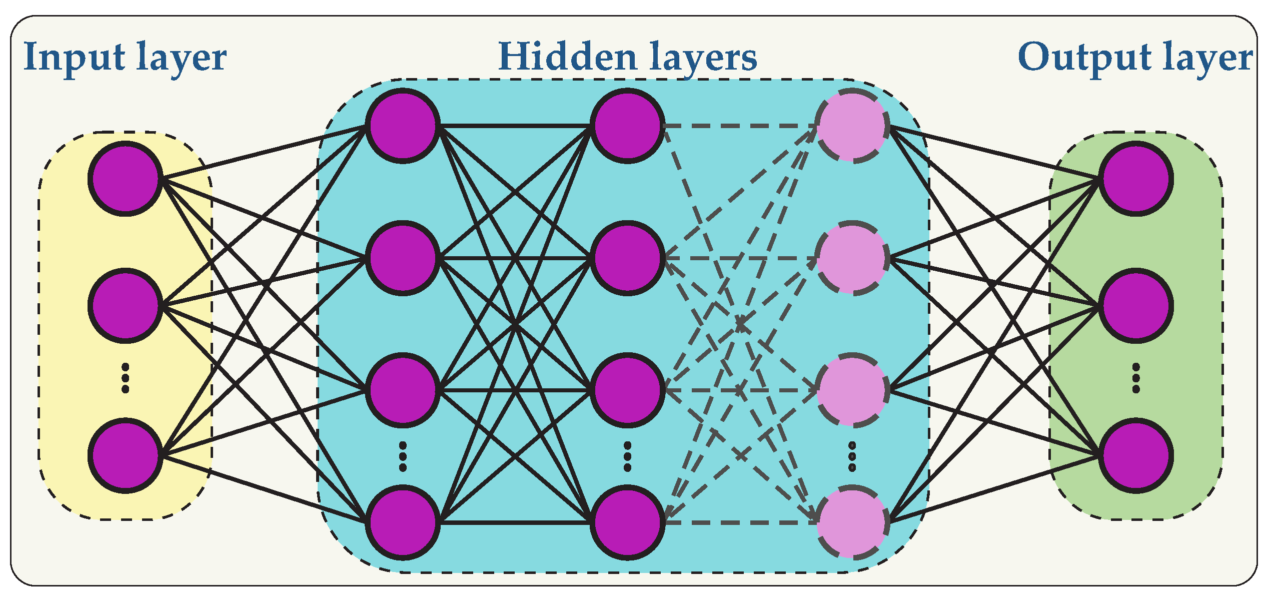
2.2. Deep Neural Networks
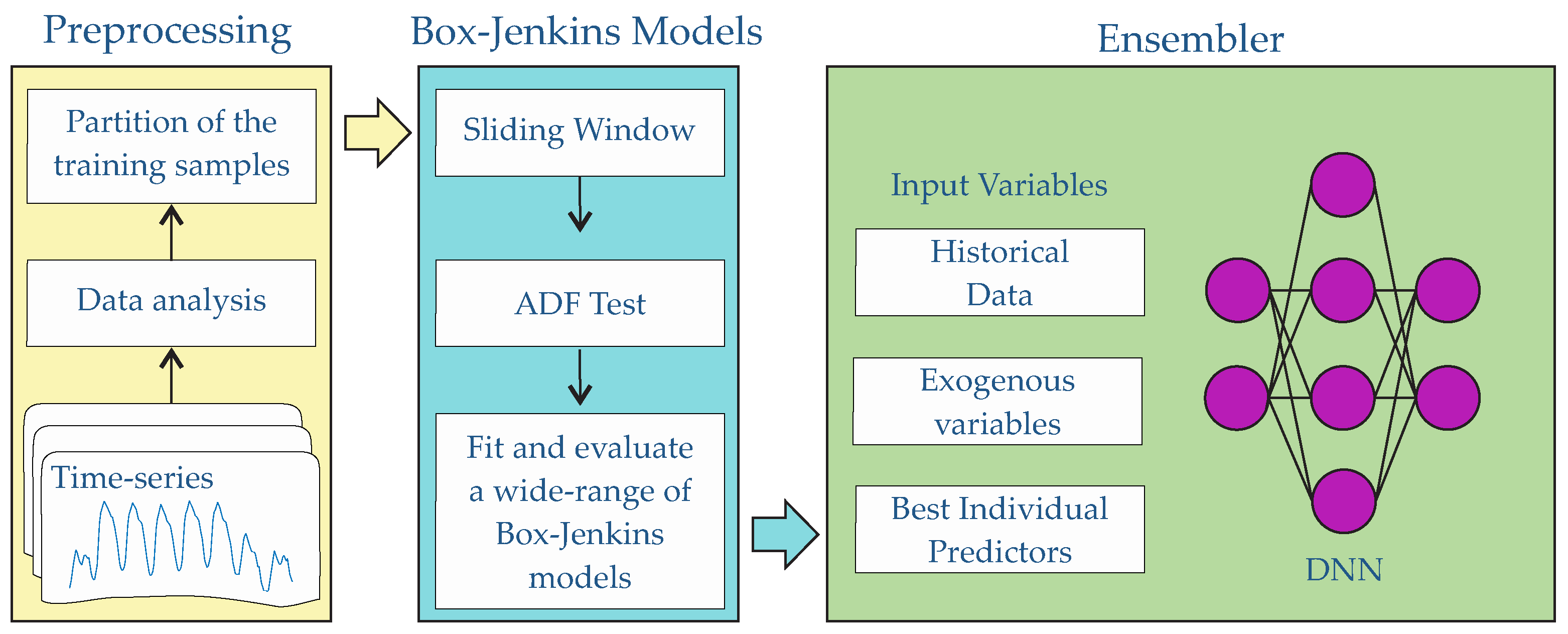
3. Proposed Methodology
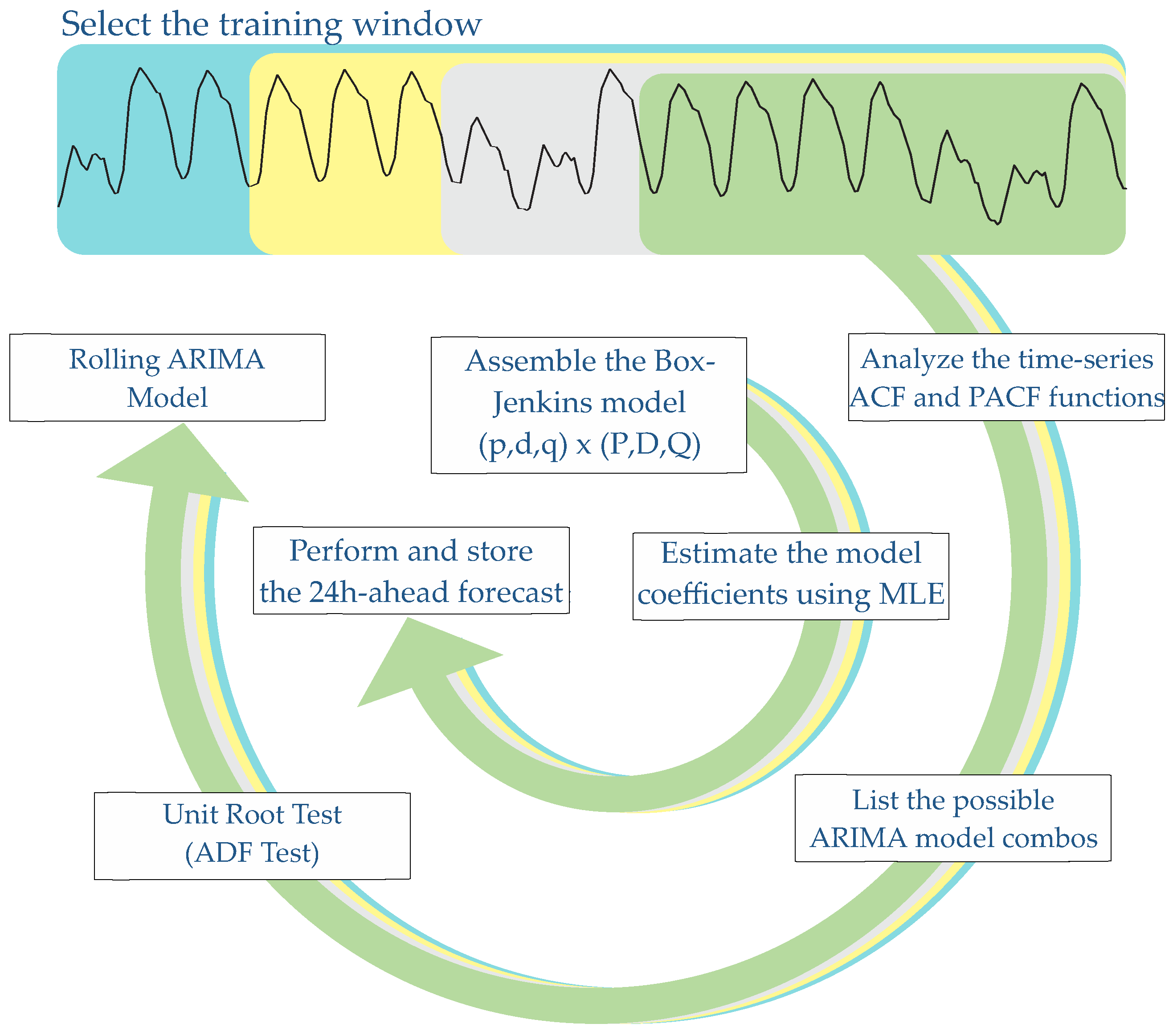
3.1. Prediction Models: ARIMA Forecasters
3.2. Ensembler DFNN
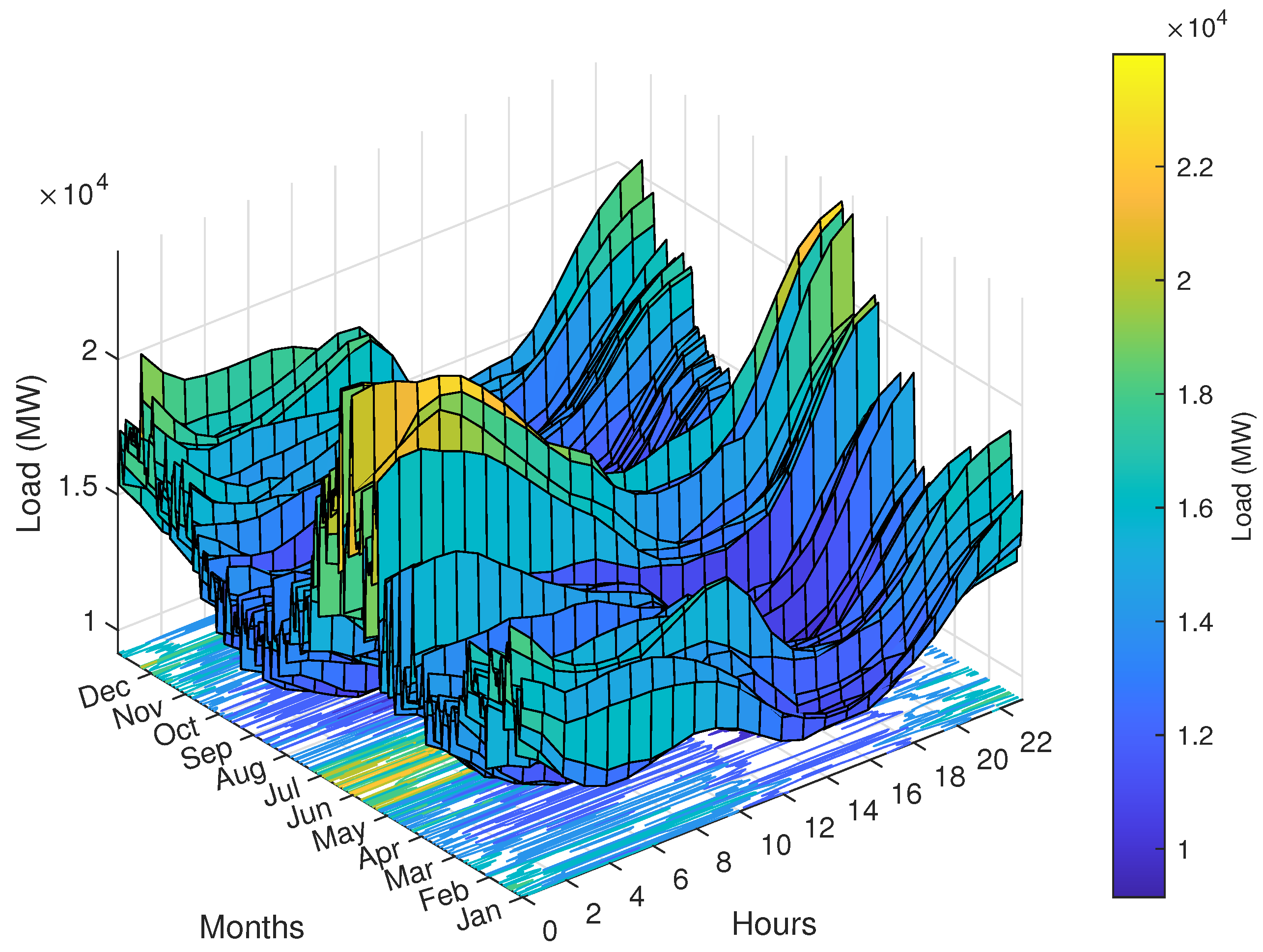
4. Case Study
5. Results
6. Conclusions
Author Contributions
Funding
Data Availability Statement
Acknowledgments
Conflicts of Interest
Nomenclature
| weighted sum in neuron j; | |
| ACF | Autocorrelation function; |
| ADF | Augmented Dickey–Fuller test; |
| ANFIS | Adaptive neuro-fuzzy inference system; |
| ARIMA | Autoregressive integrated moving average; |
| ARMA | Autoregressive moving average; |
| Bias connection in neuron j; | |
| B | Backshift operator; |
| Bayesian information criterion; | |
| CNN | Convolutional neural network; |
| d | Degree of nonseasonal integration; |
| D | Degree of seasonal integration; |
| DBN | Deep belief network; |
| DFNN | Deep feedforward neural network; |
| DL | Deep learning; |
| DNN | Deep neural network; |
| Exogenous (DNN) input variable at time-step t; | |
| ELM | Extreme learning machine; |
| Activation cost in neuron j; | |
| Composite function illustrating the DNN cascaded nature; | |
| GARCH | Generalized autoregressive conditional heteroskedasticity; |
| GRU | Gated recurrent unit (neural network); |
| Output of an arbitrary hidden layer l receiving an input x; | |
| ISO-NE | New England indepedent system operator (regional transmission); |
| k | Number of (ARIMA) model parameters; |
| l | Arbitrary DNN hidden layer; |
| Actual (real) load at time-step i; | |
| LSTM | Long short-term memory (neural network); |
| (Final) forecasted load at time-step i; | |
| L | Number of DNN hidden layers; |
| m | Number of neurons in layer l; |
| MAPE | Mean absolute percentage error; |
| ML | Machine Learning; |
| MLP | Multilayer perceptron (neural network); |
| ModPerfF | Modified DNN performance error; |
| MSE | Mean squared error; |
| MSW | Mean squared weights; |
| n | Number of neurons/inputs in layer ; |
| Number of time-series samples/observations; | |
| Number of training samples; | |
| Number of testing samples; | |
| Number of DNN weights (total); | |
| N-BEATS | Neural basis expansion analysis for interpretable time series forecasting; |
| DNN output layer (linear) transfer function; | |
| p | Nonseasonal autoregressive polynomial degree; |
| P | Seasonal autoregressive polynomial degree; |
| PACF | Partial autocorrelation function; |
| q | Nonseasonal moving average polynomial degree; |
| Q | Seasonal moving average polynomial degree; |
| RMSE | Root mean squared error; |
| RNN | Recurrent neural network; |
| Residual sum square error; | |
| SARIMA | Seasonal autoregressive integrated moving average; |
| SCG | Scaled conjugate gradient algorithm; |
| STLF | Short-term load forecast; |
| SVM | Support-vector machine; |
| VMD | Variational mode decomposition; |
| Input signal from neuron i (to neuron j); | |
| Maximum input time-series value; | |
| Minimum input time-series value; | |
| Pre-processed normalized input value; | |
| X | Generic time-series; |
| XGB | Extreme gradient boosting; |
| Output response from an arbitrary neuron j; | |
| Output forecast of the different forecasters j; | |
| Slope of the linear output transfer function ; | |
| Set of training samples (in months) to model the forecasters; | |
| Lagged error term at time-step t; | |
| Generalization ratio | |
| Nonseasonal moving average coefficient at lag i; | |
| Seasonal moving average coefficient at lag i; | |
| Constant (ARIMA model) term; | |
| Sigmoid transfer function; | |
| Nonseasonal autoregressive coefficient at lag i; | |
| Seasonal autoregressive coefficient at lag i; | |
| Generic time-series sample at time-step t; | |
| Connection weight between neurons/input i and j. |
Appendix A
- (1)
- INIT;
- (2)
- GET and format the electric ISO-NE load data and relevant calendar and exogenous variables;
- (3)
- COMPUTE the load time-series analysis using ACF and PACF;
- (4)
- LIST a series of suitable ARIMA and SARIMA models based on the correlation analysis (with different thresholds) and known seasonalities;
- (5)
- SET load datasets with different windowing (number of past observations), as expressed in variable ;
- (6)
- CALCULATE the ADF test to check for stationarity and decide upon the required degree of time-series integration, d;
- (7)
- FIT the different pool of Box-Jenkins models (base learners/forecasters) to the different training windows of (endogenous) load samples;
- (8)
- COMPUTE BIC, i.e., Equation (7), to select the 3 best Box-Jenkins models for each training window;
- (9)
- DETERMINE and store the 24 h-ahead STLF with the Box-Jenkins models selected in the previous step (totaling 15 base learners) in a rolling (ARIMA or SARIMA) scheme;
- (10)
- DEFINE the input dataset format, concatenating the ARIMA forecasts with the ruled relevant exogenous and calendar variables, and its correspondent target value. Forming a pair of training sample to desired output (24 h ahead);
- (11)
- NORMALIZE the input data using Equation (8), the training, validation and testing datasets (sets of input and target samples is prepared);
- (12)
- DEFINE the different set of DFNN hyperparameters for a regression task:
- (i)
- Architecture: 3 hidden layers with sizes (number of neurons) [20,10,5], respectively;
- (ii)
- Optimizer (Learning Algorithm): SCG;
- (iii)
- The training and validation performance is evaluated using modPerfF (Equation (9));
- (iv)
- Train to Validation Ratio: 70% to 30%;
- (v)
- Sigmoid transfer function in the hidden layers;
- (vi)
- Linear transfer function in the (last) output layer;
- (13)
- SET number of runs = 50;
- (14)
- FOR each run out of number of runs;
- (i)
- TRAIN the DFNN in an offline process with updated weights after each test week is predicted;
- (a)
- WHILE (iterations < 2500);
- (I)
- IF (validation error stops decreasing and counter < 50);
- (A)
- Counter += 1;
- (II)
- ELSE IF (counter 50);
- (A)
- BREAK loop;
- (III)
- ELSE;
- (A)
- Counter = 0;
- (ii)
- COMPUTE the STLF using the trained DFNN in the testing dataset;
- (iii)
- STORE the predicted loads and the respective forecasting;
- (vi)
- UPDATE the training and validation input dataset to include the most recently predicted data and return to (i);
- (v)
- IF (no more test weeks to predict);
- (a)
- BREAK loop;
- (15)
- END
References
- Mishra, M.; Nayak, J.; Naik, B.; Abraham, A. Deep learning in electrical utility industry: A comprehensive review of a decade of research. Eng. Appl. Artif. Intell. 2020, 96, 104000. [Google Scholar] [CrossRef]
- Xu, F.Y.; Cun, X.; Yan, M.; Yuan, H.; Wang, Y.; Lai, L.L. Power Market Load Forecasting on Neural Network with Beneficial Correlated Regularization. IEEE Trans. Ind. Inform. 2018, 3203, 1–10. [Google Scholar] [CrossRef]
- Xie, Y.; Ueda, Y.; Sugiyama, M. A Two-Stage Short-Term Load Forecasting Method Using Long Short-Term Memory and Multilayer Perceptron. Energies 2021, 14, 5873. [Google Scholar] [CrossRef]
- El-Hendawi, M.; Wang, Z. An ensemble method of full wavelet packet transform and neural network for short term electrical load forecasting. Electr. Power Syst. Res. 2020, 182, 106265. [Google Scholar] [CrossRef]
- Ghelardoni, L.; Member, S.; Ghio, A.; Anguita, D.; Member, S. Energy Load Forecasting Using Empirical Mode Decomposition and Support Vector Regression. IEEE Trans. Smart Grid 2013, 4, 549–556. [Google Scholar] [CrossRef]
- Yuansheng, H.; Shenhai, H.; Jiayin, S. A Novel Hybrid Method for Short-Term Power Load Forecasting. J. Electr. Comput. Eng. 2016, 2016, 2165324. [Google Scholar] [CrossRef]
- Feinberg, E.a.; Genethliou, D. Applied Mathematics for Restructured Electric Power Systems. IEEE Trans. Autom. Control 2005, 50, 269–285. [Google Scholar] [CrossRef]
- Rueda, F.D.; Suárez, J.D.; Torres, A.d.R. Short-Term Load Forecasting Using Encoder-Decoder WaveNet: Application to the French Grid. Energies 2021, 14, 2524. [Google Scholar] [CrossRef]
- Acakpovi, A.; Ternor, A.T.; Asabere, N.Y.; Adjei, P.; Iddrisu, A.S. Time Series Prediction of Electricity Demand Using Adaptive Neuro-Fuzzy Inference Systems. Math. Probl. Eng. 2020, 2020, 4181045. [Google Scholar] [CrossRef]
- Bento, P.; Pombo, J.; Calado, M.; Mariano, S. Optimization of neural network with wavelet transform and improved data selection using bat algorithm for short-term load forecasting. Neurocomputing 2019, 358, 53–71. [Google Scholar] [CrossRef]
- Moon, J.; Kim, Y.; Son, M.; Hwang, E. Hybrid Short-Term Load Forecasting Scheme Using Random Forest and Multilayer Perceptron. Energies 2018, 11, 3283. [Google Scholar] [CrossRef] [Green Version]
- Semero, Y.K.; Zhang, J.; Zheng, D. EMD–PSO–ANFIS-based hybrid approach for short-term load forecasting in microgrids. IET Gener. Transm. Distrib. 2020, 14, 470–475. [Google Scholar] [CrossRef]
- Ceperic, E.; Ceperic, V.; Baric, A. A strategy for short-term load forecasting by support vector regression machines. IEEE Trans. Power Syst. 2013, 28, 4356–4364. [Google Scholar] [CrossRef]
- Yuan, T.L.; Jiang, D.S.; Huang, S.Y.; Hsu, Y.Y.; Yeh, H.C.; Huang, M.N.L.; Lu, C.N. Recurrent Neural Network Based Short-Term Load Forecast with Spline Bases and Real-Time Adaptation. Appl. Sci. 2021, 11, 5930. [Google Scholar] [CrossRef]
- Bento, P.; Pombo, J.; Mariano, S.; Calado, M.d.R. Short-Term Load Forecasting using optimized LSTM Networks via Improved Bat Algorithm. In Proceedings of the 2018 International Conference on Intelligent Systems (IS), Funchal, Portugal, 25–27 September 2018; pp. 351–357. [Google Scholar] [CrossRef]
- Ciechulski, T.; Osowski, S. High Precision LSTM Model for Short-Time Load Forecasting in Power Systems. Energies 2021, 14, 2983. [Google Scholar] [CrossRef]
- Wu, W.; Liao, W.; Miao, J.; Du, G. Using Gated Recurrent Unit Network to Forecast Short-Term Load Considering Impact of Electricity Price. Energy Procedia 2019, 158, 3369–3374. [Google Scholar] [CrossRef]
- Yeom, C.U.; Kwak, K.C. Short-Term Electricity-Load Forecasting Using a TSK-Based Extreme Learning Machine with Knowledge Representation. Energies 2017, 10, 1613. [Google Scholar] [CrossRef]
- Yu, Y.; Ji, T.Y.; Li, M.S.; Wu, Q.H. Short-term Load Forecasting Using Deep Belief Network with Empirical Mode Decomposition and Local Predictor. In Proceedings of the IEEE Power and Energy Society General Meeting, Portland, OR, USA, 5–10 August 2018. [Google Scholar] [CrossRef]
- Mansoor, M.; Grimaccia, F.; Leva, S.; Mussetta, M. Comparison of echo state network and feed-forward neural networks in electrical load forecasting for demand response programs. Math. Comput. Simul. 2021, 184, 282–293. [Google Scholar] [CrossRef]
- Acharya, S.K.; Wi, Y.M.; Lee, J. Short-Term Load Forecasting for a Single Household Based on Convolution Neural Networks Using Data Augmentation. Energies 2019, 12, 3560. [Google Scholar] [CrossRef] [Green Version]
- Oreshkin, B.N.; Dudek, G.; Pełka, P.; Turkina, E. N-BEATS neural network for mid-term electricity load forecasting. Appl. Energy 2021, 293, 116918. [Google Scholar] [CrossRef]
- Sowinski, J. The Impact of the Selection of Exogenous Variables in the ANFIS Model on the Results of the Daily Load Forecast in the Power Company. Energies 2021, 14, 345. [Google Scholar] [CrossRef]
- Jin, Y.; Guo, H.; Wang, J.; Song, A. A Hybrid System Based on LSTM for Short-Term Power Load Forecasting. Energies 2020, 13, 6241. [Google Scholar] [CrossRef]
- Khashei, M.; Hajirahimi, Z. A comparative study of series arima/mlp hybrid models for stock price forecasting. Commun. Stat.-Simul. Comput. 2018, 48, 2625–2640. [Google Scholar] [CrossRef]
- Nazar, M.S.; Fard, A.E.; Heidari, A.; Shafie-khah, M.; Catalão, J.P. Hybrid model using three-stage algorithm for simultaneous load and price forecasting. Electr. Power Syst. Res. 2018, 165, 214–228. [Google Scholar] [CrossRef]
- Nie, H.; Liu, G.; Liu, X.; Wang, Y. Hybrid of ARIMA and SVMs for short-term load forecasting. Energy Procedia 2011, 16, 1455–1460. [Google Scholar] [CrossRef] [Green Version]
- Büyükşahin, Ü.Ç.; Ertekin, Ş. Improving forecasting accuracy of time series data using a new ARIMA-ANN hybrid method and empirical mode decomposition. Neurocomputing 2019, 361, 151–163. [Google Scholar] [CrossRef] [Green Version]
- Guo, W.; Che, L.; Shahidehpour, M.; Wan, X. Machine-Learning based methods in short-term load forecasting. Electr. J. 2021, 34, 106884. [Google Scholar] [CrossRef]
- Shen, Y.; Ma, Y.; Deng, S.; Huang, C.J.; Kuo, P.H. An Ensemble Model based on Deep Learning and Data Preprocessing for Short-Term Electrical Load Forecasting. Sustainability 2021, 13, 1694. [Google Scholar] [CrossRef]
- Massaoudi, M.; Refaat, S.S.; Chihi, I.; Trabelsi, M.; Oueslati, F.S.; Abu-Rub, H. A novel stacked generalization ensemble-based hybrid LGBM-XGB-MLP model for Short-Term Load Forecasting. Energy 2021, 214, 118874. [Google Scholar] [CrossRef]
- Salmi, T.; Kiljander, J.; Pakkala, D. Stacked Boosters Network Architecture for Short-Term Load Forecasting in Buildings. Energies 2020, 13, 2370. [Google Scholar] [CrossRef]
- Lai, C.S.; Mo, Z.; Wang, T.; Yuan, H.; Ng, W.W.; Lai, L.L. Load forecasting based on deep neural network and historical data augmentation. IET Gener. Transm. Distrib. 2020, 14, 5927–5934. [Google Scholar] [CrossRef]
- Sharma, R.R.; Kumar, M.; Maheshwari, S.; Ray, K.P. EVDHM-ARIMA-Based Time Series Forecasting Model and Its Application for COVID-19 Cases. IEEE Trans. Instrum. Meas. 2021, 70. [Google Scholar] [CrossRef]
- Zhao, Z.; Wang, C.; Nokleby, M.; Miller, C.J. Improving short-term electricity price forecasting using day-ahead LMP with ARIMA models. In Proceedings of the IEEE Power and Energy Society General Meeting, Chicago, IL, USA, 16–20 July 2018; pp. 1–5. [Google Scholar] [CrossRef] [Green Version]
- Chen, W.; Xu, H.; Chen, Z.; Jiang, M. A novel method for time series prediction based on error decomposition and nonlinear combination of forecasters. Neurocomputing 2021, 426, 85–103. [Google Scholar] [CrossRef]
- Rajagukguk, R.A.; Ramadhan, R.A.A.; Lee, H.J. A Review on Deep Learning Models for Forecasting Time Series Data of Solar Irradiance and Photovoltaic Power. Energies 2020, 13, 6623. [Google Scholar] [CrossRef]
- Shrestha, A.; Mahmood, A. Review of deep learning algorithms and architectures. IEEE Access 2019, 7, 53040–53065. [Google Scholar] [CrossRef]
- Shinozaki, T.; Watanabe, S. Structure discovery of deep neural network based on evolutionary algorithms. In Proceedings of the 2015 IEEE International Conference on Acoustics, Speech and Signal Processing (ICASSP), South Brisbane, Australia, 19–24 April 2015; pp. 4979–4983. [Google Scholar] [CrossRef]
- Witten, I.H.; Frank, E.; Hall, M.A.; Pal, C.J. Chapter 10—Deep learning. In Data Mining: Practical Machine Learning Tools and Techniques; Witten, I.H., Frank, E., Hall, M.A., Pal, C.J.B.T.D.M.F.E., Eds.; chapter Deep learn; Morgan Kaufmann: Burlington, MA, USA, 2017; pp. 417–466. [Google Scholar] [CrossRef]
- Jagait, R.K.; Fekri, M.N.; Grolinger, K.; Mir, S. Load Forecasting Under Concept Drift: Online Ensemble Learning with Recurrent Neural Network and ARIMA. IEEE Access 2021, 98992–99008. [Google Scholar] [CrossRef]
- Barak, S.; Sadegh, S.S. Forecasting energy consumption using ensemble ARIMA–ANFIS hybrid algorithm. Int. J. Electr. Power Energy Syst. 2016, 82, 92–104. [Google Scholar] [CrossRef] [Green Version]
- Ganaie, M.A.; Hu, M.; Tanveer, M.; Suganthan, P.N. Ensemble Deep Learning: A Review. arXiv 2021, arXiv:2104.02395. [Google Scholar]
- Prado, F.; Minutolo, M.C.; Kristjanpoller, W. Forecasting based on an ensemble Autoregressive Moving Average–Adaptive neuro–Fuzzy inference system–Neural network–Genetic Algorithm Framework. Energy 2020, 197, 117159. [Google Scholar] [CrossRef]
- Hyndman, R.J.; Kostenko, A.V.; Hyndman, R.; Kostenko, A.V. Minimum Sample Size requirements for Seasonal Forecasting Models. Foresight Int. J. Appl. Forecast. 2007, 6, 12–15. [Google Scholar]
- Shetty, J.; Shobha, G. An ensemble of automatic algorithms for forecasting resource utilization in cloud. In FTC 2016—Proceedings of Future Technologies Conference; Institute of Electrical and Electronics Engineers Inc.: San Francisco, CA, USA, 2017; pp. 301–306. [Google Scholar] [CrossRef]
- Van Giang, T.; Debusschere, V.; Bacha, S. One week hourly electricity load forecasting using Neuro-Fuzzy and Seasonal ARIMA models. IFAC Proc. Vol. 2012, 45, 97–102. [Google Scholar] [CrossRef]
- Møller, M.F. A scaled conjugate gradient algorithm for fast supervised learning. Neural Netw. 1993, 6, 525–533. [Google Scholar] [CrossRef]
- Delavar, M.R. Hybrid machine learning approaches for classification and detection of fractures in carbonate reservoir. J. Pet. Sci. Eng. 2022, 208, 109327. [Google Scholar] [CrossRef]
- England, I.N. ISO New England—Energy, Load, and Demand Reports. 2021. Available online: https://www.iso-ne.com/isoexpress/web/reports/load-and-demand (accessed on 26 July 2021).


| Prediction Model/Test Month | 16 February | 16 April | 16 August | 16 October |
|---|---|---|---|---|
| ARIMA Forecaster 1 | 4.36 | 6.34 | 5.26 | 4.37 |
| ARIMA Forecaster 2 | 4.79 | 7.28 | 5.25 | 5.37 |
| ARIMA Forecaster 3 | 4.87 | 7.40 | 5.51 | 5.32 |
| ARIMA Forecaster 4 | 4.93 | 7.49 | 5.73 | 5.20 |
| ARIMA Forecaster 5 | 4.93 | 7.55 | 5.48 | 5.14 |
| Ensemble DFNN | 3.67 | 6.19 | 4.82 | 3.75 |
| Prediction Model/Test Month | 16 February | 16 April | 16 August | 16 October |
|---|---|---|---|---|
| ARIMA Forecaster 1 | 737.3 | 1266.6 | 983.7 | 774.5 |
| ARIMA Forecaster 2 | 840.7 | 1443.5 | 978.6 | 937.7 |
| ARIMA Forecaster 3 | 859.8 | 1446.4 | 1034.6 | 916.7 |
| ARIMA Forecaster 4 | 857.6 | 1454.9 | 1067.2 | 891.7 |
| ARIMA Forecaster 5 | 860.5 | 1454.6 | 1034.1 | 915.9 |
| Ensemble DFNN | 649.4 | 1254.1 | 883.3 | 634.7 |
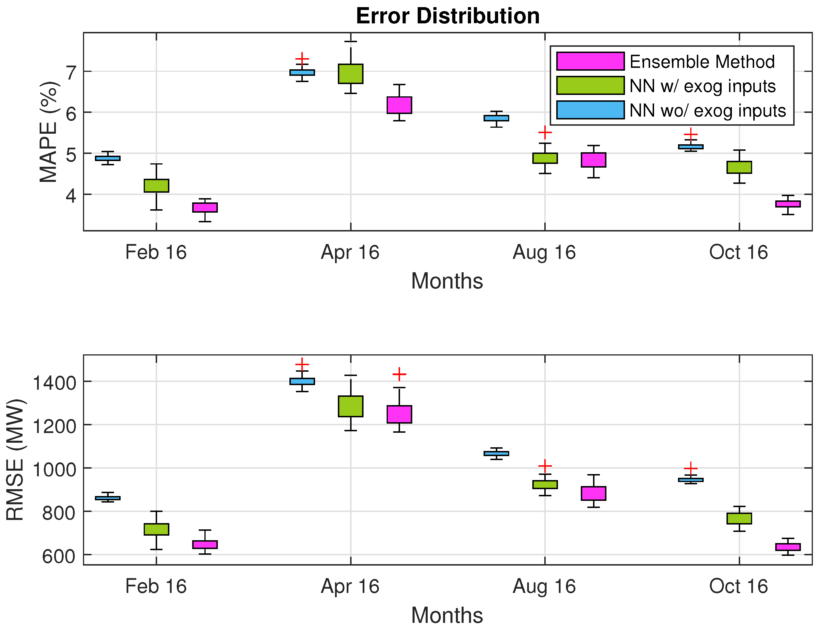
| Method/Test Month | 16 February | 16 April | 16 August | 16 October |
|---|---|---|---|---|
| R-SVM | 4.71 | 8.15 | 5.39 | 5.67 |
| NN wo/ Exog | 4.87 | 6.96 | 5.85 | 5.16 |
| NN w/ Exog | 4.22 | 6.99 | 4.89 | 4.66 |
| Ensemble DFNN | 3.67 | 6.19 | 4.82 | 3.75 |
| Method/Test Month | 16 February | 16 April | 16 August | 16 October |
|---|---|---|---|---|
| R-SVM | 769.5 | 1492.7 | 914.6 | 958.2 |
| NN wo/ Exog | 860.1 | 1400.5 | 1066.8 | 945.2 |
| NN w/ Exog | 717.8 | 1278.6 | 923.5 | 769.2 |
| Ensemble DFNN | 649.4 | 1254.1 | 883.3 | 634.7 |
Publisher’s Note: MDPI stays neutral with regard to jurisdictional claims in published maps and institutional affiliations. |
© 2021 by the authors. Licensee MDPI, Basel, Switzerland. This article is an open access article distributed under the terms and conditions of the Creative Commons Attribution (CC BY) license (https://creativecommons.org/licenses/by/4.0/).
Share and Cite
Bento, P.M.R.; Pombo, J.A.N.; Calado, M.R.A.; Mariano, S.J.P.S. Stacking Ensemble Methodology Using Deep Learning and ARIMA Models for Short-Term Load Forecasting. Energies 2021, 14, 7378. https://0-doi-org.brum.beds.ac.uk/10.3390/en14217378
Bento PMR, Pombo JAN, Calado MRA, Mariano SJPS. Stacking Ensemble Methodology Using Deep Learning and ARIMA Models for Short-Term Load Forecasting. Energies. 2021; 14(21):7378. https://0-doi-org.brum.beds.ac.uk/10.3390/en14217378
Chicago/Turabian StyleBento, Pedro M. R., Jose A. N. Pombo, Maria R. A. Calado, and Silvio J. P. S. Mariano. 2021. "Stacking Ensemble Methodology Using Deep Learning and ARIMA Models for Short-Term Load Forecasting" Energies 14, no. 21: 7378. https://0-doi-org.brum.beds.ac.uk/10.3390/en14217378