A Modified Multiple-Mixing-Cell Method with Sub-Cells for MMP Determinations

Abstract

Minimum miscible pressure (MMP) is an essential design parameter of gas flooding for enhanced oil recovery (EOR) applications. Researchers have developed a number of methods for MMP computations, including the analytical methods, the slim-tube simulation method, and the multiple-mixing-cell (MMC) method. Among these methods, the MMC method is widely accepted for its simplicity, robustness, and moderate computational cost An important version of the MMC method is the Jaubert et al. method which has a much lower computational cost than the slim-tube simulation method. However, the original Jaubert et al. method suffers several drawbacks. One notable drawback is that it cannot be applied to the scenario where the oil-gas MMP is lower than the saturation pressure of the crude oil. In this work, we present a modified MMC method that is more versatile and robust than the original version. Our method can handle the scenario where the oil-gas MMP is lower than the saturation pressure of the crude oil. Besides, we propose a modified MMC model that can reduce the computational cost of MMP estimations. This modified model, together with a newly proposed pressure search algorithm, increases the MMP estimation accuracy of the modified method. We demonstrate the good performance of the modified MMC method by testing it in multiple case studies. A good agreement is obtained between the MMPs calculated by the modified method and the tie-line-based ones from the literature.

1. Introduction

Gas flooding is one enhanced oil recovery (EOR) method that injects CO₂ or other gases into reservoirs to displace oil. It has been researched and applied in the fields since the 1950s [1,2,3]. Since 2006, the gas flooding projects account for more than half of all the EOR projects worldwide [4], showing the utmost importance of this EOR method. To obtain a high recovery factor in a gas flooding project, the injected gas should develop miscibility with the in-situ oil [5]. This minimum pressure, at which the miscibility is reached, is defined as the minimum miscibility pressure (MMP). MMP is an essential design parameter of gas flooding projects.

There are various experimental and computational methods to determine MMP. Experimental methods include the rising bubble experiment method [6,7], the vanishing interfacial tension method [8,9], and the slim-tube method [5,10,11]. Among these methods, the slim-tube method is an industrially accepted experimental method. Its procedure is briefly summarized as follows. At a given pressure level (such as the bubble point pressure of the reservoir oil), we conduct a displacement test by injecting gas into a slim-tube apparatus to displace oil. We then record the oil recovery factor when the injected gas volume reaches 1.2 times the slim-tube pore volume (PV). This displacement test is repeated at increased pressure levels. The oil recovery factors corresponding to 1.2 PV injection are plotted against pressure. The MMP can be finally determined as the pressure at the inflection point of the trend line exhibited by the data points. Slim-tube experiments are not only easy to implement but also capable of providing reliable MMP measurements [12]. However, as an experimental method, the slim-tube method is inevitably costlier and more time-consuming than its counterpart slim-tube simulation method.

The slim-tube simulation method [13,14,15] is a straightforward computational method to estimate MMP by simulating the slim-tube experiments in a fine one-dimensional (1D) compositional simulation model. Such a 1D model consists of a row of multiple grid cells. To increase the estimation accuracy of the numerical model, an important treatment is to calculate the extrapolated infinite-cell recovery factor. For example, as in Høier’s implementation [15], three numerical displacement tests are conducted by 100-, 200- and 500-grid-cell models, respectively, to record three recovery factors. The three recovery factors are used to fit a pre-defined curve model and the fitted curve is extrapolated to obtain the infinite-cell recovery factor. This exercise is then repeated at different pressure levels. Similar to the real slim-tube experiments, the final step is to identify the inflection point in the plot of recovery factor vs. pressure.

The slim-tube simulation method can be further simplified as the multiple-mixing-cell (MMC) method [16] where a grid cell is simplified as a mixing cell. Specifically, in each mixing cell, flow dynamics are neglected and only the isobaric-isothermal (PT) equilibria of oil and gas mixtures are considered. Similarly, this MMC method consists of two key parts. The first part is the 1D numerical MMC model (a simplified slim-tube simulation model) that can generate the infinite-cell recovery factors, while the second part is the specific pressure search algorithm for MMP determination. Originally, this MMC model was designed to perform oil vaporization calculations by Cook et al. [17]. It was later modified by Metcalfe et al. [18] and Pederson et al. [19] to study miscibility mechanisms. Jaubert et al. [16] successfully applied this MMC model for MMP estimations. In the following discussion, we refer to this method as the J-MMC method and the corresponding numerical model as the J-MMC model.

Figure 1 shows a simple schematic of the J-MMC model. In Figure 1, we have used 5 mixing cells and 5 batches, forming a 5 × 5 matrix. The topology of the matrix is controlled by three key parameters, i.e., cell number (analogous to grid number), batch number (analogous to time step number), and gas-oil mixing ratio ($GOR$). In the matrix, each row represents the 1D model at one batch (time step). Note that the parameter $GOR$ is irrelevant to the conventional definition in the oil and gas industry, but it can be interpreted as the “injection speed” of gas in the 1D model. Figure 2 shows the simulation workflow of the 1D model at a certain batch and at a specified pressure. As shown in Figure 2, a specified volume of gas is “injected” and mixed with the oil in the 1st cell. In the mixing at the 1st cell, the ratio of the injected-gas volume to the original oil volume in the 1st cell is defined as $GOR$. To calculate the fluid’s volume at equilibrium after mixing, one PT phase equilibrium calculation is conducted. At equilibrium, the fluid in the 1st cell will expand and the “excessive” volume as defined by Jaubert et al. [16] will be transferred to the 2nd cell and contact the oil therein. Figure 3 shows the detailed procedure to transfer the excessive fluid [16]. As shown in Figure 3, if the fluid at equilibrium appears as a single phase (scenario 1), directly transfer the excessive volume; if the fluid at equilibrium appears as two phases and the liquid phase volume is smaller than the cell volume (scenario 2), transfer a part of the vapor phase; if the fluid at equilibrium appears as two phases and the liquid phase volume is larger than the cell volume (scenario 3), transfer the whole vapor phase and a part of the liquid phase. We repeat such transferring calculations until reaching the last cell from which the excessive volume is finally “produced”. Subsequently, we proceed to the next-batch calculations by using the same amount of injected gas. The calculation is completed until a total of 1.2 PV of gas is injected. Eventually, the oil recovery factor of this n-cell model at a specified pressure level can be determined as the summation of the produced oil volumes from all the batches divided by the original oil volume in the n-cells, both at the standard condition.

In the J-MMC method, different from the previous slim-tube simulation method, we only need to conduct one simulation run by using the largest number of required cells to calculate the infinite-cell recovery factor. For example, as stated by Jaubert et al. [16], only a simulation run using a 500-cell model needs to be conducted, from which the 50-, 100-, 200-, and 500-cell recovery factors can be obtained at the same time. These four data points are used to fit a linear model (i.e., a straight line) and the fitted model is extrapolated to calculate the infinite-cell recovery factor. Besides, a pressure search algorithm is executed to determine three pressure points to calculate the corresponding infinite-cell recovery factors. Then, the three points of infinite-cell recovery factor vs. pressure are used for fitting an exponential model. Finally, the pressure corresponding to a 97% recovery factor is determined as MMP [16].

Except for the J-MMC method, Ahmadi and Johns [20] proposed another state-of-the-art MMC method, and its computational efficiency is further improved by Zhao et al. [21]. Similarly, we refer to this method as the AJ-MMC method and the corresponding numerical model as the AJ-MMC model. Different from the J-MMC method, the AJ-MMC method applies the zero-tie-line-length criterion to find the MMP at which the corresponding minimum tie-line length is zero. Such methodology originates from the analytical method-of-characteristics (MOC) method [22,23,24,25,26,27]. One notable innovation of the AJ-MMC method is that the authors design a “triangular” MMC model that can calculate all the tie-line lengths numerically at a specified pressure. Besides, a new pressure search algorithm is implemented to update pressure values until the MMP is determined. On the one hand, Ahmadi and Johns [20] prove that the estimation accuracy of the AJ-MMC method is as high as the MOC method. On the other hand, the AJ-MMC method can only handle two-phase equilibria. The corresponding three-phase version of the AJ-MMC method [28] shows that the zero-tie-line-length criterion is not strictly valid in a three-phase displacement case.

Both the J-MMC and AJ-MMC methods can estimate MMPs in a faster way than the slim-tube experiments and the slim-tube simulations. But only the J-MMC method can provide the recovery factor information as the AJ-MMC model contains non-physical mechanisms. Another important feature of the J-MMC method is that the procedure to transfer the excessive fluid volume is physical and general, making it naturally extendable to handle three hydrocarbon phases. This indicates that this method can be used to estimate MMPs of three-phase displacement cases with little modifications.

However, to the best of our knowledge, the MMP estimation accuracy of the J-MMC method has yet been compared with the tie-line-based methods (the AJ-MMC and MOC methods). Our first work is to compare the original J-MMC method to the tie-line-based methods. Appendix A shows the detailed comparison. We obtain two observations from the comparative analysis. Firstly, the MMPs obtained from the J-MMC method are less accurate than the ones from the tie-line-based methods. Secondly, the pressure search algorithm of the J-MMC method fails in several cases, including the case where the oil-gas MMP is lower than the saturation pressure of the crude oil.

Therefore, the motivation of this paper is to propose a modified MMC method based on the original J-MMC method to increase its robustness, improve its estimation accuracy, and enhance its computational accuracy. This paper is organized as follows. In “Methodology”, we provide a modified MMC model and a new pressure search algorithm. In “Results and Discussion”, we verify the improvements of the modified method and apply the method to estimate the MMPs of several two-phase displacement cases. The MMP estimates are compared with the ones calculated by the original J-MMC method, tie-line-based methods, and slim-tube methods. Finally, the conclusions are drawn in “Conclusions”.

2. Methodology

The new MMC method contains two key parts, i.e., the modified MMC model, and a new pressure search algorithm. The PT phase equilibrium calculation algorithm is the kernel of the MMC method for calculating the number of equilibrium phases, their compositions, and volumes after mixing. We implement a stepwise algorithm workflow where a stability test is implemented before the flash calculation to provide a good initial guess for the flash calculation [29,30]. For both the stability test and flash calculation, we use a sequential strategy that combines the successive substitution (SS), the second-order Newton’s method, and a switch-back option when infeasible conditions are encountered in Newton’s method [31]. Note that the initial guesses used in the stability test are summarized by Pan et al. [32], and we use the Peng-Robinson equation of state [33] in all the phase equilibrium calculations. In the following subsections, the modified MMC model and the pressure search algorithm will be introduced in detail.

2.1. Modified MMC Model

There are three core assumptions in the MMC model [34]:

• Perfect mixing in each cell;
• No physical dispersions between cells;
• No capillary force.

The original J-MMC model is a one-dimensional model with three key parameters, i.e., $nc$ (cell number), $nb$ (batch number), and $GOR$ (gas-oil mixing ratio). As shown in Figure 2, one PT calculation is conducted in each cell. In a complete simulation run, the total number of PT algorithm calls ($N_{PT}$) is given by [16],

$$N_{PT}=nc\times nb=nc\times \frac{1.2\times nc}{GOR}=\frac{1.2\times n{c}^2}{GOR}.$$

(1)

In Equation (1), $N_{PT}$ is a function of both $nc$ and $GOR$. $N_{PT}$ can be largely increased with a decrease in $GOR$. For example, $nc$ and $GOR$ are set to 500 and 1/3 in the original J-MMC model, resulting in a large $N_{PT}$.

Our modification is to get rid of changing $GOR$ (set as a constant of one) and introduce a new mechanism of dividing one cell into sub-cells with the same volume. In other words, we keep the “injection speed” unchanged but enlarge the model size to increase the computational accuracy. Figure 4 illustrates the displacement workflow of the two-sub-cell model at a certain batch. As shown in Figure 4, the sub-cells are used to transfer excessive fluid within one original mixing cell, and the simulation workflow keeps unaltered. As one PT calculation is conducted in each sub-cell, the total number of PT algorithm calls ($N_{PT}^{\prime }$) in the modified model is given by,

$$N_{PT}^{\prime }=\left(2\times nc\right)\times nb=\left(2\times nc\right)\times \left(1.2\times nc\right)=2.4\times n{c}^2.$$

(2)

Equation (2) shows that $N_{PT}^{\prime }$ equals two-third of $N_{PT}$ when $GOR=1/3$. The use of two sub-cells in each cell leads to a better mixing efficiency because there are two mixing events taking place in each cell. Although the number of PT calculations will be increased due to the use of two sub-cells, it will be shown in the “Results and Discussion” section that the use of two sub-cells leads to a more accurate MMP determination without imposing an additional computational load.

In one simulation run, the $n{c}_j$-cell recovery factor at a specified pressure $p$ ($rf\left(n{c}_j,p\right)$) is expressed as,

$$rf\left(n{c}_j,p\right)=\frac{{{\displaystyle \sum }}_{i=1}^{nb}{V}_{oil,sc}^{prod}\left(i,n{c}_j,p\right)}{n{c}_j\times V_{oil,sc}^0\left(p\right)},$$

(3)

where $n{c}_j\in NC=\left\{n{c}_1,n{c}_2,n{c}_3,\dots \right\}$ and $NC$ is a user-defined integer array; $V_{oil,sc}^{prod}\left(i,nc,p\right)$ represents the produced oil volume at the $nc$ cell, at the ith batch, and at the standard condition; $V_{oil,sc}^0\left(p\right)$ is the initial oil volume in each cell at the standard condition. Each $n{c}_j$ in the array $NC$ corresponds to a recovery factor to be calculated by Equation (3). We can then obtain the dataset $\left\{R{F}^T, N{C}^T\right\}$, where

$$RF=\left\{rf\left(n{c}_1,p\right),rf\left(n{c}_2,p\right),\dots ,rf\left(n{c}_j,p\right),\dots |n{c}_j\in NC\right\}$$

(4)

Using this dataset, we can estimate the infinite-cell recovery factor by fitting a second-order polynomial model ($r{f}^{poly}\left(nc,p\right)$) in terms of $1/\sqrt{nc}$ as given below [15],

$$r{f}^{poly}\left(nc,p\right)=A+\frac{B}{\sqrt{nc}}+\frac{C}{nc}$$

(5)

where A, B, and C are three to-be-determined coefficients.

The fitted model is extrapolated to yield the infinite-cell recovery factor ($r{f}^{\infty }\left(p,NC\right)$),

$$r{f}^{\infty }\left(p,NC\right)=A.$$

(6)

As pointed out by Jaubert et al. [16], we need only a single run by using $nc=\max \left\{n{c}_j|n{c}_j\in NC\right\}$ to obtain the complete data set $\left\{R{F}^T, N{C}^T\right\}$.

2.2. Pressure Search Algorithm

We define a modified fitting model to describe how recovery factor ($r{f}^{\infty }$) changes with an increase in pressure. This model is given by,

$$D\times {\left(1-r{f}^{\infty }\left(p,NC\right)\right)}^E+F=\ln \left(p\right),$$

(7)

where D, E, and F are three to-be-determined coefficients, and the value of $E$ becomes an estimation of MMP when $r{f}^{\infty }\left(p,NC\right)\to 1$. The corresponding dataset used for fitting Equation (7) is $\{{(R{F}^{\infty })}^T, P^T\}$, where

$$R{F}^{\infty }=\left\{r{f}^{\infty }\left(p_1,NC\right),r{f}^{\infty }\left(p_2,NC\right),\dots ,r{f}^{\infty }\left(p_n,NC\right),\dots |p_n\in P\right\}.$$

(8)

Another two definitions used in the algorithm are, respectively, the numerical slope $k$ and the fitting weight $w$ for pressure $p_n$. The slope $k$ is defined as,

$$k\left(p_n,NC\right)=\frac{r{f}^{\infty }\left(p_n,NC\right)-r{f}^{\infty }\left(p_{n-1},NC\right)}{p_n-p_{n-1}}, n\ge 2$$

(9)

The weight $w$ is defined in the weighted-curve-fitting objective function. The objective function (S) is expressed as [35],

$$S={\displaystyle \sum }_{i=1}^n{w}_i{\left(r{f}_i^{\infty }-{\widehat{rf}}_i^{\infty }\right)}^2,$$

(10)

where $r{f}_i^{\infty }$ is the infinite-cell recovery factor calculated by Equation (6) and ${\widehat{rf}}_i^{\infty }$ is the modeled infinite-cell recovery factor calculated by Equation (7). Note that we can define the unweighted-fitting objective function simply by setting all weights in Equation (10) to one. In Equation (10), the weight $w$ is defined as [35],

$$w\left(p_n,NC\right)=\frac{1}{{\sigma }^2\left(RF\right)},$$

(11)

where ${\sigma }^2$ represents the variance of array $RF$.

Presented below is the detailed numerical procedure for MMP determination:

• Estimate roughly the bubble point pressure $p_b$, define $N{C}_0$ with small cell numbers (such as $N{C}_0=\left\{10,20,30\right\}$) and calculate $r{f}^{\infty }\left(p_b,N{C}_0\right)$. $p_b$ can be rounded as a multiple of 10;
• Take $p_b$ as the first point and build an initial dataset $\{{(R{F}_{init}^{\infty })}^T, P_{init}^T\}$ that satisfies $P_{init}=\left\{\dots , p_b-\Delta p, p_b, p_b+\Delta p, \dots \right\}$ with a constant difference $\Delta p$ and $\forall p\in P_{init}\left(0.1<r{f}^{\infty }\left(p,N{C}_0\right)<1\right)$. The initial value of $\Delta p$ can be 10 bar;
• Using the definition in Equation (9), calculate the slopes from the second point in the initial dataset and find the slope increasing dataset $\{{(R{F}_{incr}^{\infty })}^T, P_{incr}^T\}$ that satisfies the following conditions: $P_{incr}\subseteq P_{init}$ and $\forall p_n\in P_{incr}\left(k\left(p_n,N{C}_0\right)\le k\left(p_{n+1},N{C}_0\right), n\ge 2\right)$ and $\forall p\in P_{incr}(r{f}^{\infty }\left(p,N{C}_0\right)>0.3)$. If the number of elements in $P_{incr}$ is smaller than 5, decrease $\Delta p$ and go back to step 2;
• Define the slope increasing interval as $\left[\min \left(P_{incr}\right),\max \left(P_{incr}\right)\right]$ and choose $NC$ with relatively larger cell numbers (such as $NC=\left\{100,200,300,400\right\}$) to increase the computational accuracy;
• Select three pressure values ($p_1$, $p_2$, and $p_3$) that increase with a constant interval inside the bottom 25% of $\left[\min \left(P_{incr}\right),\max \left(P_{incr}\right)\right]$. The value of the interval can be $\Delta p$ or $\Delta p/2$. The three points are the initial points in a new dataset $\{{(R{F}_{incr1}^{\infty })}^T, P_{incr1}^T\}$ to calculate the infinite-cell recovery factors with $NC$. Fit these three consecutive points at these three pressures using Equation (7) to obtain an initial MMP ($MM{P}_{init, 1}$). Determine a new pressure as follows,

$$p_{3+1}=p_{2+1}+\frac{1}{3}\times \left(MM{P}_{init, 1}-p_{2+1}\right)$$

(12)

If $r{f}^{\infty }\left(p_{3+1},NC\right)-r{f}^{\infty }\left(p_{2+1},NC\right)>10\%$, reset $p_{3+1}$ as,

$$p_{3+1}=p_{2+1}+\frac{1}{3}\times \left(p_{3+1}-p_{2+1}\right)$$

(13)

Once the fourth pressure $p_{3+1}=p_4$ is obtained, start the iteration as follows. In this iteration, we specify $i$ as the index of the initial MMPs ($MM{P}_{init, i}$, $i\ge 2$). Fit the three consecutive points at $p_i$, $p_{1+i}$, and $p_{2+i}$ using Equation (7) to obtain a new initial MMP ($MM{P}_{init, i}$). Determine a new pressure as follows,

$$p_{3+i}=p_{2+i}+\frac{1}{3}\times \left(MM{P}_{init, i}-p_{2+i}\right);$$

(14)

If $r{f}^{\infty }\left(p_{3+i},NC\right)-r{f}^{\infty }\left(p_{2+i},NC\right)>10\%$, reset $p_{3+i}$ as,

$$p_{3+i}=p_{2+i}+\frac{1}{3}\times \left(p_{3+i}-p_{2+i}\right);$$

(15)

Add the pair $\left\{r{f}^{\infty }\left(p_{3+i},NC\right),p_{3+i}\right\}$ into the dataset $\{{(R{F}_{incr1}^{\infty })}^T, P_{incr1}^T\}$ iteratively until $r{f}^{\infty }\left(p_{3+i},NC\right)>0.8$ or $k\left(p_{3+i}\right)\le k\left(p_{2+i}\right)$. Such a pressure searching algorithm is inspired by the work by Ahmadi and Johns [20].

6.

Build the final estimation dataset $\{{(R{F}_{est}^{\infty })}^T, P_{est}^T\}$ that satisfies $P_{est}\subseteq P_{incr1}$ and $\forall p\in P_{est}(0.3<r{f}^{\infty }\left(p,NC\right)<0.8)$.

7.

Fit Equation (7) with $\{{(R{F}_{est}^{\infty })}^T, P_{est}^T\}$ and the corresponding weights defined by Equation (11), and then calculate $MM{P}_1$ (the 1st MMP estimation) by extrapolating the fitted model to $r{f}^{\infty }=1$; Fit Equation (7) again with $\{{(R{F}_{est}^{\infty })}^T, P_{est}^T\}$ directly without applying any weights, and calculate $MM{P}_2$ (the 2nd MMP estimation) by extrapolating the fitted model to $r{f}^{\infty }=1$. Determine the final MMP as the mean of the two previous MMP estimations.

In summary, the overall procedure consists of four essential steps. First, we obtain an initial dataset of $r{f}^{\infty }$ vs. $p$ using small cell numbers ($N{C}_0$). Secondly, we determine the slope increasing interval over which the slope defined by Equation (9) is monotonically increasing. Thirdly, we build a new dataset of $r{f}^{\infty }$ vs. $p$ using larger cell numbers ($NC$). Fourthly, we determine MMP by fitting Equation (7) with the new dataset of $r{f}^{\infty }$ vs. $p$. Figure 5 shows the flowchart of the detailed numerical procedure.

3. Results and Discussion

We use the same five example cases (cases a to e) as examined in Appendix A. In the following calculations, we use a two-sub-cell MMC model. We firstly demonstrate how the modified method leads to improved recovery factor calculations. Then we list the MMPs estimated by the modified method and compare them with the ones from the literature, especially the ones calculated by the tie-line-based methods.

3.1. Improvements on Recovery Factor Calculations

At a specified pressure level, we calculate the recovery factors by using the modified model with required cell numbers. These recovery factors are used to estimate the infinite-cell recovery factor. There are two improvements, namely, one on the recovery factor calculations, and one on the infinite-cell recovery factor estimations.

To show the improvement in the recovery factor calculations, we compare the recovery factors at specified pressures and cell numbers calculated by four different models. These models are the modified J-MMC model and the three J-MMC models with different GORs.

Table 1. Calculated recovery factors at specified cell numbers and 130 bar for case a by different MMC models.

MMC Model	Cell Number
	25	50	75	100	150	200	300	400
Modified J-MMC model	0.45605	0.47488	0.48161	0.48481	0.48764	0.48882	0.48985	0.49032
J-MMC model (GOR = 1.0)	0.44261	0.46645	0.47591	0.48070	0.48522	0.48722	0.48891	0.48964
J-MMC model (GOR = 1/2)	0.45136	0.47223	0.47986	0.48353	0.48682	0.48823	0.48945	0.49003
Original J-MMC model (GOR = 1/3)	0.45462	0.47422	0.48116	0.48442	0.48730	0.48853	0.48963	0.49016

and

Table 2. Calculated recovery factors at specified cell numbers and 180 bar for case b by different MMC models.

MMC Model	Cell Number
	25	50	75	100	150	200	300	400
Modified J-MMC model	0.36942	0.39890	0.41314	0.42177	0.43171	0.43719	0.44304	0.44622
J-MMC model (GOR = 1.0)	0.35236	0.38529	0.40144	0.41152	0.42362	0.43062	0.43826	0.44236
J-MMC model (GOR = 1/2)	0.36433	0.39505	0.40991	0.41898	0.42953	0.43540	0.44168	0.44508
Original J-MMC model (GOR = 1/3)	0.36891	0.39873	0.41305	0.42170	0.43161	0.43704	0.44286	0.44603

list the comparison of the recovery factors of case a at 130 bar and case b at 180 bar, respectively. On each row of the two tables (i.e., for the same model), a model with a larger model size yields a larger (i.e., more accurate) recovery factor. This statement also holds for the three J-MMC models on one column (i.e., at a fixed cell number). But the recovery factor calculated by the modified model is the largest one on each column. This indicates that the modified model is more accurate than the original J-MMC model under the same GOR of 1/3. By comparing the total numbers of PT calculations runs, it is apparent that the modified model is also more cost-efficient than the original J-MMC model.

We then conduct another comparative study to illustrate the improvement of the infinite-cell recovery factor estimations. In this comparison, we fit the new second-order polynomial model and the original linear model (from the J-MMC method) in four different scenarios. The four scenarios are 157.37 bar of case a, 160 bar of case b, 212.43 bar of case b, 89.07 bar of case c. In each scenario, we calculate eight recovery factors using the 100-, 200-, …, 800-cell models. For each curve fitting exercise, the first four recovery factors (i.e., the recovery factors calculated by the 100-, 200-, 300-, and 400-cell models) are used for fitting, while the last four (i.e., the recovery factors calculated by the 500-, 600-, 700-, and 800-cell models) are used to evaluate the performance of the fitting. Figure 6, Figure 7, Figure 8 and Figure 9 show the curve fitting results for the four scenarios. In Figure 6, the fitted linear and polynomial models are similar, and both can well predict the last four recovery factors. In Figure 7, Figure 8 and Figure 9, the fitted polynomial model better predicts the recovery factors marked by squares. In general, the fitted curves by the second-order polynomial model demonstrate a better fitting quality. Thus, the new fitting model can provide more reasonable predictions on infinite-cell recovery factors.

3.2. Example Calculation

We use the modified MMC method to estimate the MMPs of the five two-phase displacement cases. To begin with, we presented an example calculation of case a to show how to implement the new pressure search algorithm.

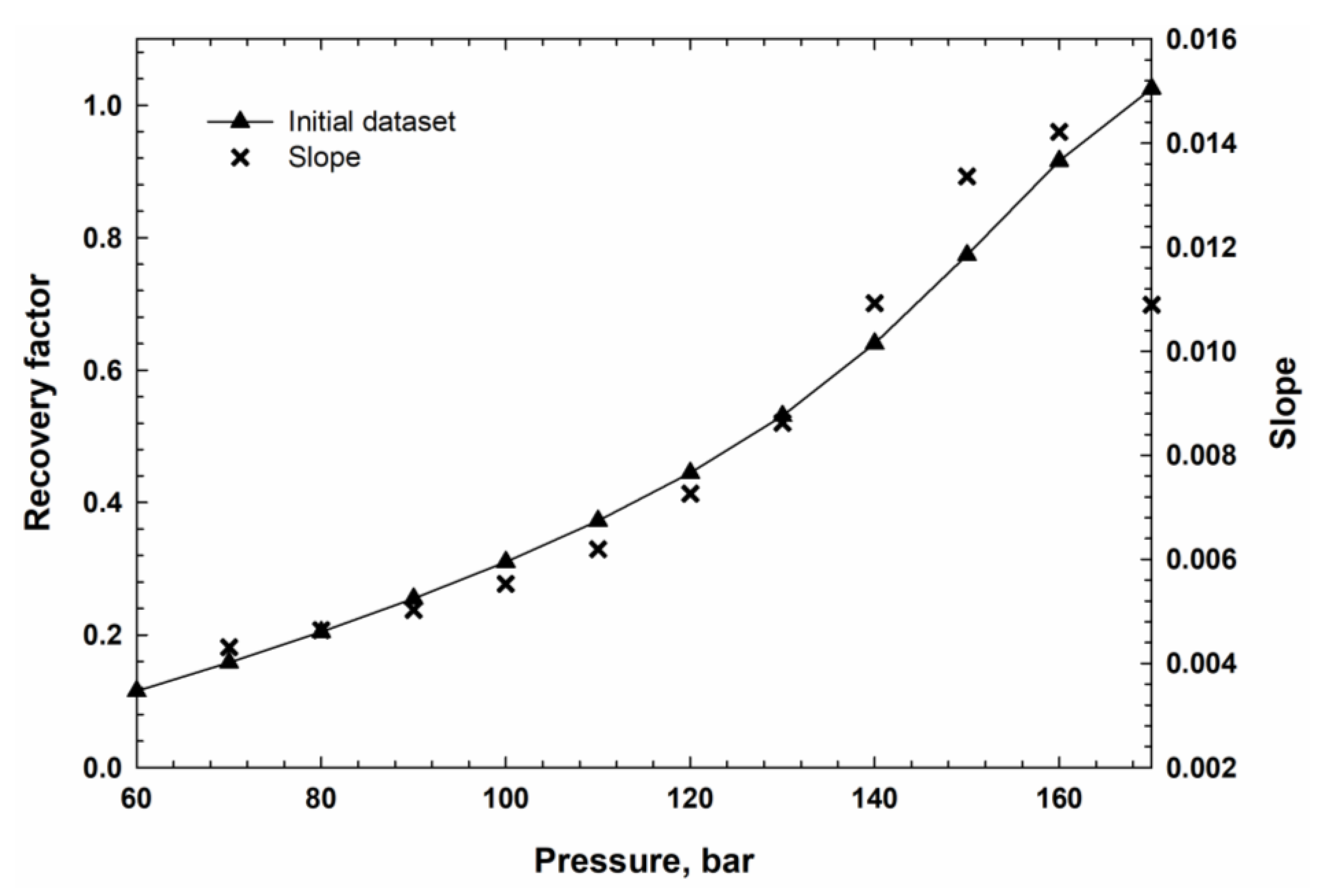
The first step of the algorithm is to generate the dataset of $r{f}^{\infty }$ vs. $p$ with the cell number $N{C}_0$ and determine the slope increasing interval. Figure 10 shows this dataset ($\{{(R{F}_{init}^{\infty })}^T, P_{init}^T\}$) represented by a line with triangles and the corresponding slopes represented by crosses. We define the interval, where the slope is monotonically increasing, as the slope increasing interval. As shown in Figure 10, the slope increasing interval is determined as [100 bar, 160 bar]. Next, we select three pressure values in the interval to initiate the calculation of a new dataset of $r{f}^{\infty }$ vs. $p$ with the cell number $NC$. After calculating $r{f}^{\infty }$ at the selected three pressures, we iteratively identify the additional pressure levels using Equations (14) and (15). Using the updated pressure levels, we further calculate $r{f}^{\infty }$ until the termination criteria are satisfied. Figure 11 shows the new dataset of $r{f}^{\infty }$ vs. $p$ and the related data to determine the final MMP. As shown in Figure 11, we obtain two fitted curves with weighted and unweighted fittings, respectively (see Equations (10) and (11)). The two curves will intersect with the horizontal line corresponding to a recovery factor of 1. The two intersection points will be the two MMPs estimated by the modified J-MMC method. The MMPs estimated from the weighted and unweighted fittings are labeled as the 1st and the 2nd MMP estimations, respectively. The final MMP is determined as 155.74 bar, which is the mean value of the two MMP estimations.

3.3. Comparison of MMPs Estimated by Different Methods

Using the same procedure, we estimate the MMPs of the remaining four cases. The MMPs calculated by the modified J-MMC method, together with the values calculated by the original J-MMC method, are compared with the ones from the literature.

Table 3. MMP estimations (bar) calculated by the modified MMC and the original J-MMC methods and the comparison with the ones from the literature.

Case Index	$\mathbf{M}\mathbf{M}{\mathit{P}}_1$	$\mathbf{M}\mathbf{M}{\mathbf{P}}_2$	Average	Jaubert et al. Method [16]	Reference MMP Values
					MOC	MMC Method by Ahmadi and Johns [20]	Slim-Tube
a	155.10	156.37	155.74	166.92	158.37 [24]	158.78 ± 0.28 [20]	-
b	211.18	212.43	211.80	225.38 A	213.39 [25]	219.80 ± 3.45 [20]	215.46 [36]
c	89.63	89.18	89.41	90.16 A	89.49 ± 0.14 [20]	89.49 ± 0.45 [20]	-
d	154.09	154.55	154.32	165.67 B	158.78 [25]	-	154.014 [36]
e	529.58	532.10	530.84	550.18	526.18 [25]	-	518.78 ± 7.09 [15]

A: The oil-gas MMPs (estimated by the modified MMC method) are lower than the oil saturation pressures. The original J-MMC method fails to detect MMPs for these two cases. We resolve this issue by manually selecting three pressures that are used to calculate the infinite-cell recovery factor. B: The oil-gas MMP (estimated by the modified MMC method) is higher than the oil saturation pressure. The original J-MMC method fails to detect MMP for this case. We resolve this issue by manually selecting three pressures that are used to calculate the infinite-cell recovery factor.

shows the detailed comparison result.

Table 4. Relative errors * of the MMPs calculated by the modified J-MMC method and the original J-MMC method in terms of the reference MMPs from the literature.

Case Index	Relative Error by the Modified J-MMC Method			Relative Error by the Original J-MMC Method
	MOC	MMC Method by Ahmadi and Johns [20]	Slim-Tube	MOC	MMC Method by Ahmadi and Johns [20]	Slim-Tube
a	1.66%	(1.91 ± 0.18)%	-	5.40%	(5.13 ± 0.18)%	-
b	0.75%	(3.64 ± 1.57)%	1.70%	5.62%	(2.54 ± 1.57)%	4.60%
c	(0.09 ± 0.16)%	(0.09 ± 0.50)%	-	(0.75 ± 0.16)%	(0.75 ± 0.50)%	-
d	2.81%	-	0.20%	4.34%	-	7.57%
e	0.89%	-	(2.32 ± 1.36)%	4.56%	-	(6.05 ± 1.36)%

* $\mathrm{Relative} \mathrm{error}=\frac{\left|\mathrm{MMP} \mathrm{calculated} \mathrm{in} \mathrm{this} \mathrm{work} - \mathrm{MMP} \mathrm{from} \mathrm{the} \mathrm{literature}\right|}{\mathrm{MMP} \mathrm{from} \mathrm{the} \mathrm{literature}}\times 100\%$. The MMPs from the literature refer to the MMPs reported in the last three columns in Table 3.

shows the relative errors of the MMPs calculated by the modified J-MMC method and the original J-MMC method. The relative errors are obtained by treating the reference MMPs from the literature as true values. As shown in Table 3 and Table 4, the new MMPs calculated by the modified method are in better agreement with the ones calculated by the AJ-MMC method, the MOC method, and the slim-tube methods. Besides, our method successfully determines the MMPs of cases b to d, while the original J-MMC method fails to predict MMPs for these three cases (as shown in

Table A1. Detailed MMP estimation results by the J-MMC method [16] and the comparison with the MMPs estimated by the AJ-MMC and MOC methods.

Case Index	Estimated Bubble Point Pressure (bar)	Estimated First Contact Miscibility Pressure (bar)	Calculated Pressures (bar)	Extrapolated Recovery Factor	Select/Reject	Pressure Search Algorithm Succeeds?	Estimated MMP (bar)	Reference MMP (bar)
								MOC	MMC Method by Ahmadi and Johns [20]
a	56	177	56	0.0945	Reject	Yes	166.92	158.37 [24]	158.78 ± 0.28 [20]
			80.2	0.2019	Select
			104.4	0.3251	Select
			128.6	0.4880	Select
b	224	492	224	0.9468	Select	NO	225.38	213.39 [25]	219.80 ± 3.45 [20]
			277.6	1.0248	Reject
			170.4	0.4023	Select
			197.2	0.6295	Select
c	105	127	105	1.0322	Reject	NO	90.16	89.49 ± 0.14 [20]	89.49 ± 0.45 [20]
			100.6	1.0419	Reject
			96.2	1.0361	Reject
			91.8	1.0030	Reject
			87.4	0.4332	Select
			89.6	0.8280	Select
			88.5	0.4843	Select
d	105	373	105	0.3639	Select	NO	165.67	158.78 [25]	-
			158.6	0.8655	Select
			212.2	1.0199	Reject
			51.4	0.0000	Reject
			131.8	0.5585	Select
e	248	908	248	0.0290	Reject	Yes	550.18	526.18 [25]	-
			380	0.2886	Select
			512	0.7155	Select
			644	1.0054	Reject
			446	0.4628	Select

). Note that the oil-gas MMPs of cases b and c (estimated by the modified MMC method) are lower than the oil saturation pressures, while the oil-gas MMP of case d (estimated by the modified MMC method) is higher than the oil saturation pressure.

4. Conclusions

In this work, we develop a modified MMC method based on the original J-MMC method. The following conclusions are drawn:

• We propose a new MMC model where one mixing cell is divided into two sub-cells with the same volume. With this feature, the new MMC model can estimate the infinite-cell recovery factor in a more accurate and cost-efficient manner.
• A new pressure search algorithm is proposed to provide a reliable MMP estimation. This algorithm can handle the case where the oil-gas MMP is lower than the saturation pressure of the crude oil.
• The case studies demonstrate that the MMPs calculated by the modified J-MMC method are in better agreement with the ones from the literature, indicating that the modified J-MMC method is more accurate than the original one.
• The method assumes a maximum of two hydrocarbon phases will be encountered when displacing the oil. It is logical to further extend the application of the new method to handle the cases where three-phase equilibria will be encountered. But such a J-MMC method would require a robust three-phase equilibrium calculation algorithm. This topic will be pursued in our future works.

References

- Stalkup, F.I. Status of miscible displacement. J. Pet. Technol. 1983, 35, 815–826. [Google Scholar] [CrossRef]
- Ali, M.; Dahraj, N.U.; Haider, S.A. Study of asphaltene precipitation during CO2 injection in light oil reservoirs. In Proceedings of the SPE/PAPG Pakistan section Annual Technical Conference, Islamabad, Pakistan, 24–25 November 2015. [Google Scholar]
- Ali, M.; Al-Anssari, S.; Shakeel, M.; Arif, M.; Dahraj, N.U.; Iglauer, S. Influence of miscible CO2 flooding on wettability and asphaltene precipitation in Indiana lime stone. In Proceedings of the SPE/IATMI Asia Pacific Oil & Gas Conference and Exhibition, Jakarta, Indonesia, 17–19 October 2017. [Google Scholar]
- IEA. 2019. Available online: https://www.iea.org/data-and-statistics/charts/number-of-eor-projects-in-operation-globally-1971-2017 (accessed on 21 August 2021).
- Yellig, W.F.; Metcalfe, R.S. Determination and prediction of CO2 minimum miscibility pressures (includes associated paper 8876). J. Pet. Technol. 1980, 32, 160–168. [Google Scholar] [CrossRef]
- Christiansen, R.L.; Haines, H.K. Rapid measurement of minimum miscibility pressure with the rising-bubble apparatus. SPE Res. Eng. 1987, 2, 523–527. [Google Scholar] [CrossRef]
- Zhou, D.; Orr, F.M., Jr. An analysis of rising-bubble experiments to determine minimum miscibility pressures. SPE J. 1998, 3, 19–25. [Google Scholar] [CrossRef]
- Rao, D.N. A new technique of vanishing interfacial tension for miscibility determination. Fluid Phase Equilibr. 1997, 139, 311–324. [Google Scholar] [CrossRef]
- Ayirala, S.C.; Rao, D.N. Comparative evaluation of a new MMP determination technique. In Proceedings of the SPE/DOE Symposium on Improved Oil Recovery, Tulsa, OK, USA, 22–26 April 2006. [Google Scholar]
- Orr, F.M.; Silva, M.K.; Lien, C.L.; Pelletier, M.T. Laboratory experiments to evaluate field prospects for CO2 flooding. J. Pet. Technol. 1982, 34, 888–898. [Google Scholar] [CrossRef]
- Li, H.; Qin, J.; Yang, D. An improved CO2–oil minimum miscibility pressure correlation for live and dead crude oils. Ind. Eng. Chem. Res. 2012, 51, 3516–3523. [Google Scholar] [CrossRef]
- Whitson, C.H.; Michael, R.B. Phase Behavior, 1st ed.; Henry, L., Ed.; Doherty Memorial Fund of AIME and Society of Petroleum Engineers Inc.: Richardson, TX, USA, 2000. [Google Scholar]
- Stalkup, F.I. Displacement behavior of the condensing/vaporizing gas drive process. In Proceedings of the SPE Annual Technical Conference and Exhibition, Dallas, TX, USA, 27–30 September 1987. [Google Scholar]
- Stalkup, F.I. Effect of gas enrichment and numerical dispersion on enriched-gas-drive predictions. SPE Res. Eng. 1990, 5, 647–655. [Google Scholar] [CrossRef]
- Høier, L. Miscibility Variations in Compositionally Grading Petroleum Reservoirs. Ph.D. Thesis, Norwegian University of Science and Technology, Trondheim, Norway, 1997. [Google Scholar]
- Jaubert, J.N.; Wolff, L.; Neau, E.; Avaullee, L. A very simple multiple mixing cell calculation to compute the minimum miscibility pressure whatever the displacement mechanism. Ind. Eng. Chem. Res. 1998, 37, 4854–4859. [Google Scholar] [CrossRef]
- Cook, A.B.; Walker, C.J.; Spencer, G.B. Realistic K values of C7+ hydrocarbons for calculating oil vaporization during gas cycling at high pressures. J. Pet. Technol. 1969, 21, 901–915. [Google Scholar] [CrossRef]
- Metcalfe, R.S.; Fussell, D.D.; Shelton, J.L. A multicell equilibrium separation model for the study of multiple contact miscibility in rich-gas drives. SPE J. 1973, 13, 147–155. [Google Scholar] [CrossRef]
- Pederson, K.S.; Fjellerup, J.; Thomassen, P.; Fredenslund, A. Studies of gas injection into oil reservoirs by a cell-to-cell simulation model. In Proceedings of the SPE Annual Technical Conference and Exhibition, New Orleans, LA, USA, 5–8 October 1986. [Google Scholar]
- Ahmadi, K.; Johns, R.T. Multiple-mixing-cell method for MMP calculations. SPE J. 2011, 16, 733–742. [Google Scholar] [CrossRef]
- Zhao, H.; Fang, Z. Improved multiple-mixing-cell method for accelerating minimum miscibility pressure calculations. SPE J. 2020, 25, 1681–1696. [Google Scholar] [CrossRef]
- Orr, F.M., Jr.; Johns, R.T.; Dindoruk, B. Development of miscibility in four-component CO2 floods. SPE Res. Eng. 1993, 8, 135–142. [Google Scholar] [CrossRef]
- Johns, R.T.; Orr, F.M., Jr. Miscible gas displacement of multicomponent oils. SPE J. 1996, 1, 39–50. [Google Scholar] [CrossRef]
- Wang, Y.; Orr, F.M., Jr. Analytical calculation of minimum miscibility pressure. Fluid Phase Equilibr. 1997, 139, 101–124. [Google Scholar] [CrossRef]
- Jessen, K.; Michelsen, M.; Stenby, E.H. Global approach for calculating minimum miscibility pressure. Fluid Phase Equilibr. 1998, 153, 251–263. [Google Scholar] [CrossRef]
- Yuan, H.; Johns, R.T. Simplified method for calculation of minimum miscibility pressure or enrichment. SPE J. 2005, 10, 416–425. [Google Scholar] [CrossRef]
- Orr, F.M., Jr. Theory of Gas Injection Processes, 1st ed.; Tie-Line Publications: Copenhagen, Denmark, 2007. [Google Scholar]
- Li, L.; Khorsandi, S.; Johns, R.T.; Ahmadi, K. Multiple-mixing-cell method for three-hydrocarbon-phase displacements. SPE J. 2015, 20, 1339–1349. [Google Scholar] [CrossRef]
- Michelsen, M.L. The isothermal flash problem. Part I. Stability test. Fluid Phase Equilibr. 1982, 9, 1–19. [Google Scholar] [CrossRef]
- Michelsen, M.L. The isothermal flash problem. Part II. Phase-split calculation. Fluid Phase Equilibr. 1982, 9, 21–40. [Google Scholar] [CrossRef]
- Petitfrere, M.; Nichita, D.V. Robust and efficient trust-region based stability analysis and multiphase flash calculations. Fluid Phase Equilibr. 2014, 362, 51–68. [Google Scholar] [CrossRef]
- Pan, H.; Connolly, M.; Tchelepi, H. Multiphase equilibrium calculation framework for compositional simulation of CO2 injection in low-temperature reservoirs. Ind. Eng. Chem. Res. 2019, 58, 2052–2070. [Google Scholar] [CrossRef]
- Robinson, D.B.; Peng, D.Y. The Characterization of the Heptanes and Heavier Fractions for the GPA Peng-Robinson Programs; Gas Processors Association: Tulsa, Oklahoma, 1978. [Google Scholar]
- Zhao, G.B.; Adidharma, H.; Towler, B.; Radosz, M. Using a multiple-mixing-cell model to study minimum miscibility pressure controlled by thermodynamic equilibrium tie lines. Ind. Eng. Chem. Res. 2006, 45, 7913–7923. [Google Scholar] [CrossRef]
- Mathworks. 2021. Available online: https://www.mathworks.com/help/curvefit/least-squares-fitting.html#bq_6ylw (accessed on 27 September 2021).
- Zick, A.A. A combined condensing/vaporizing mechanism in the displacement of oil by enriched gases. In Proceedings of the SPE Annual Technical Conference and Exhibition, New Orleans, LA, USA, 5–8 October 1986. [Google Scholar]
Figure 1.
Schematic of the original J-MMC model [16].
Figure 2.
Illustration of the simulation workflow of the J-MMC method at a certain batch. Adapted from Jaubert et al. [16].
Figure 3.
Illustration of the procedure to transfer the excessive volume from one cell to the next one in the J-MMC method. Adapted from Jaubert et al. [16].
Figure 4.
Illustration of the calculation workflow of the modified MMC model.
Figure 5.
The flowchart of the detailed numerical procedure.
Figure 6.
Comparison of the fitted curves calculated by the second-order polynomial fitting model and the linear model for infinite-cell recovery factor estimations at 157.37 bar in case a. The data points marked by circles are used to fit the two models. The correlation coefficient (R2) is calculated based on the data points marked by squares.
Figure 7.
Comparison of the fitted curves calculated by the second-order polynomial fitting model and the linear model for infinite-cell recovery factor estimations at 160 bar in case b. The data points marked by circles are used to fit the two models. The correlation coefficient (R2) is calculated based on the data points marked by squares.
Figure 8.
Comparison of the fitted curves calculated by the second-order polynomial fitting model and the linear model for infinite-cell recovery factor estimations at 212.43 bar in case b. The data points marked by circles are used to fit the two models. The correlation coefficient (R2) is calculated based on the data points marked by squares.
Figure 9.
Comparison of the fitted curves calculated by the second-order polynomial fitting model and the linear model for infinite-cell recovery factor estimations at 89.07 bar in case c. The data points marked by circles are used to fit the two models. The correlation coefficient (R2) is calculated based on the data points marked by squares.
Figure 10.
The initial infinite-cell recovery factor dataset and the calculated slopes defined by Equation (9).
Figure 11.
Calculated recovery factors and the final MMP estimation for case a. The initial dataset of vs. with the cell number is represented by the upper triangles. The final dataset of vs. with the cell number is represented by the lower triangles. The fitted curve for the 1st MMP estimation is represented by the dotted curve. The fitted curve for the 2nd MMP estimation is represented by the solid curve. The cross and star symbols represent the 1st and 2nd MMP estimations, respectively.