1. Introduction
Partial discharge (PD) is a phenomenon that commonly occurs in various electrical apparatus such as power transformers, gas insulated switchgears, and cables. It will deteriorate and damage the insulation of apparatus, causing potential hazardous power failure [
1,
2,
3,
4]. On the other hand, PD is also an indicator involving the insulation information [
5,
6,
7,
8]. In order to prevent electrical accidents from happening, PD online monitoring is very useful and necessary. For example, the ultra-high-frequency (UHF) method is one of the most frequently used techniques [
9,
10,
11,
12]. Under different measuring systems or scenarios, PD signals have different frequency characteristics and band ranges. Usually, the PD signal is a nonstationary time varying signal with short time duration, and its waveform is the damped exponential pulse (DEP) or the damped oscillatory pulse (DOP), as shown in Equation (1), whereas the parameters vary greatly, i.e., the time constant
τ,
τ1,
τ2, and central frequency
fc [
13,
14].
However, on-site measured PD signal inevitably becomes contaminated by random noises, among which Gaussian white noise and sinusoidal noise are the two main interferences [
15,
16]. Gaussian white noise is randomly distributed, and it is a probabilistic interference. The reduction method of white noise has been widely studied. For example, the well-known wavelet thresholding algorithm proposed by Donoho, as well as its various improved versions proposed later [
17,
18].
In contrast, sinusoidal noise, also known as discrete spectrum interference (DSI), is deterministic. Sinusoidal noise is usually from power line carrier communication systems and radio transmission/communication systems [
19,
20]. The noise may consist of several sinusoids, each of which have unknown parameters to be estimated, i.e., the amplitude, frequency, and phase. For example,
x =
Asin(2
πft) is a simple sinusoid signal with amplitude
A and frequency
f. It is worth noting that the frequency of sinusoidal noise may vary greatly from MHz to GHz under different scenarios.
There are also many studies regarding sinusoidal noise removal. An FFT-based approach was proposed; however, there exists difficulty in deciding the threshold [
21]. The finite impulse response (FIR) filter and notch filter were also applied, but they are non-adaptive, and some parameters have to be predetermined, and prior knowledge of the noise frequency is needed [
15,
21]. The singular value decomposition (SVD) method was also proposed in [
16]. However, this method lacks generality, due to its basic assumption about fixed number of selected singular values [
22]. In [
23], the empirical mode decomposition (EMD) method was proposed to decompose the signal into a series of intrinsic mode functions (IMFs). As an application [
14], EMD, as well as its subsequent improvements, has been applied in sinusoidal noise reduction of PD signal.
In addition, some time-frequency methods were also proposed [
24,
25]. For example, the short-time Fourier transform (STFT) [
26]. However, it cannot accurately represent the frequency information of signals. This may lead to difficulties in distinguishing wide-band PD signals from noise [
15]. Wavelet transform and wavelet package decomposition (WPD) have the same problem due to the Heisenberg uncertainty principle. Therefore, the time frequency representation (TFR) needs to be sharpened or enhanced to provide a clear and well-recognized representation. A TFR reassignment method (RM) was firstly proposed by Auger and Flandrin in [
27]. In this method, smoothed pseudo Wigner-Ville distribution is adopted, and every point (
t,
ω) is reassigned to its corresponding centroid point (
t’,
ω’). The value at point (
t’,
ω’) of the new TFR is the sum of the original values of all points reassigned to it. This reassignment leads to an enhancement of the original TFR and greatly improves its readability. Although RM works well, it is performed on the squared spectrogram modulus, and there is no straightforward reconstruction technique [
28]. Inspired by RM, researchers [
29,
30] tried to find an alternative way, while enabling direct reconstruction from TFR. Daubechies pioneered the well-known idea of synchrosqueezing transform (SST) and introduced the concept of instantaneous frequency (IF). The TFR is obtained through continuous wavelet transform (CWT) and reassigned by SST [
31].
Each sinusoid of the sinusoidal noise has fixed IF identical to its frequency. Meanwhile, nonsinusoidal signals do not have such characteristic. Nonsinusoidal signals include pure PD signal and white noise. In term of this difference, it is proposed to distinguish sinusoidal noise based on SST in this paper. After extraction of TFR with a specific IF through the inverse SST, a synthetic signal is obtained. This synthetic signal greatly reduces the energy of pure PD signal and white noise and can be regarded as the sum of the original sinusoid with the same IF and the residue. Further techniques can then be applied for refinement and remove the residue as much as possible. In this paper, the data-driven algorithm SSA proposed in [
32,
33] is adopted. In SSA, singular value decomposition (SVD) is firstly performed on the Hankel matrix of the synthetic signal, followed by a hierarchical clustering (HC) to automatically separate eigenvalues and vectors belonging to each sinusoid. The information of each sinusoid can be finally obtained. The proper combination of SST and SSA enables precise removal of the sinusoidal noise. For sake of robustness, the noise removal is operated in the frequency domain rather than the time domain by Fourier spectrum subtraction. The numerical simulation results verify the effectiveness and robustness of the proposed method.
The rest of the paper is organized as follows:
Section 2 briefly describes the principle of IF and the SST.
Section 3 introduces the recognition of IFs, information extraction of sinusoidal noise by SSA, and the consequent removal.
Section 4 and
Section 5, respectively, present a numerical simulation and an experimental study by the proposed method. Finally, conclusions are drawn in
Section 6.
2. Background and Principle of IF and SST
The observed PD signal can be described as a composite model:
where
x(
n) is the measured PD signal,
f(
n) is the pure PD signal,
s(
n) is the sinusoidal noise, and
w(
n) is Gaussian white noise with zero mean value and standard deviation
σ. The noises are independent of
f(
n), but they have different properties.
w(
n) is randomly distributed, and its values cannot be predicted. In contrast,
s(
n) is a deterministic noise whose parameters are unknown and to be estimated.
The sinusoidal noise has unknown numbers of sinusoids, and can be modelled as:
where
Nm is the number of sinusoids,
si is the
i-th sinusoid, and
Ai,
fi, and
φi are the amplitude, frequency, and initial phase of each
si, respectively. Meanwhile,
fsa is the sampling frequency.
2.1. Introduction of IF and SST
Assume a signal with the form
x(
t) =
A(
t)cos(
φ(
t)), its corresponding analytic signal can be expressed as
z(
t) =
x(
t) +
jH[
x(
t)], where H[
x(
t)] is the Hilbert transform of signal
x(
t), such that
where P.V. stands for the Cauchy principle value [
28]. Then, the canonical IF of signal
x(
t) is defined as the derivative of the angle of
z(
t):
Obviously, for any pure sinusoidal signal s(t) = Acos(2πf0t + φ0), its IF is identical to its frequency f0. However, the IF of some nonsinusoidal signals may be difficult to specify due to various choices of A(t) and φ(t).
Assume again an analytic wavelet
ψ(
t); then, the CWT of any real signal
h(
t) can be computed as Equation (6) according to Parseval’s theorem [
23]:
where
is the Fourier transform of
ψ(
t),
a is the scale, and
b is the time. By noticing Equation (7) and the fact that signal
h(
t) is real, the inverse CWT can be given as Equation (8).
where
Cψ is a constant, which is only related to
ψ(
t). A candidate IF
fs of signal
s(
t) based on the CWT is given in [
23] as Equation (9), and the CWT of signal
s(
t) is shown in Equation (10).
where
ω0 = 2π
f0, and
δ() is the delta function. Based on Equation (6) to Equation (10), it can be verified that the computed
fs of
s(
t) is identical to its canonical IF, which is an important and desired property. For any point (
a,
b) of the CWT TFR, SST reassigns it to another point (
ωs(
a,
b),
b), where
ωs = 2π
fs. As a consequence, the reassigned TFR can be computed as
By combination of Equations (8) and (11), signal
h(
t) can be obtained through inverse SST, as shown in Equation (12).
It can be seen that SST reassigns the CWT TFR, and inverse SST is able to perfectly recover the analyzed signal. This property enables recognition of signals with specific IFs and the direct reconstruction of them.
2.2. A SST Illustration of Sinusoids
Although the SST is theoretically perfect for signal analysis and reconstruction, practical implementation is of equal importance. Therefore, the choice of an analytic wavelet and the discretization for computation are necessary. In [
31], a strictly analytic wavelet is proposed, named the “bump wavelet”, which is defined in the frequency domain, as shown in Equation (13).
where
χ() is the indicator function. Discretization for CWT and SST computation can be linear or logarithmic; the latter is more efficient with no significant differences, as proposed in [
30] by Thakur. These selections are adopted in this paper for analysis in the following sections.
The discrete form of CWT and SST is shown in Equation (14).
and the discrete reconstruction of signal
h(
t) is given in Equation (15).
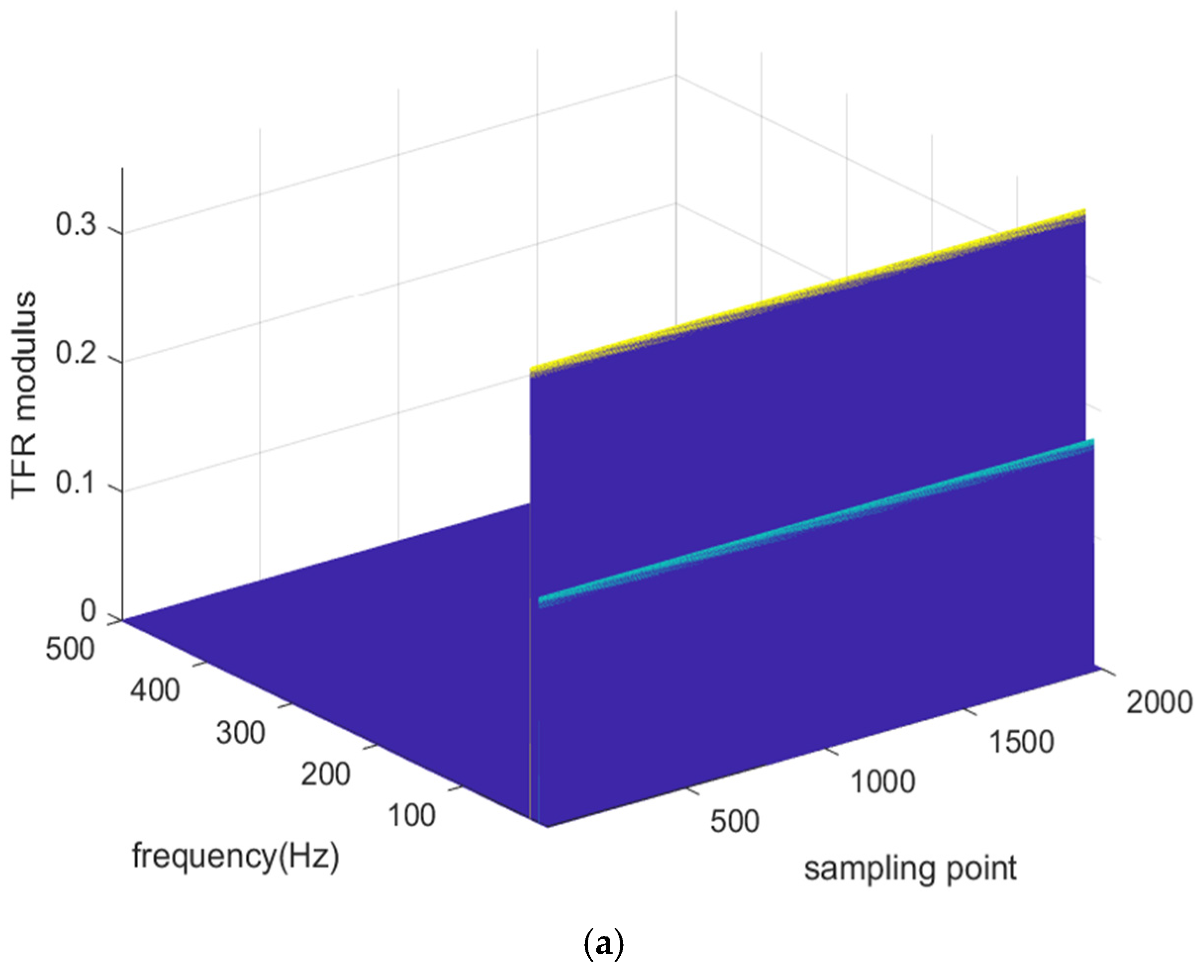
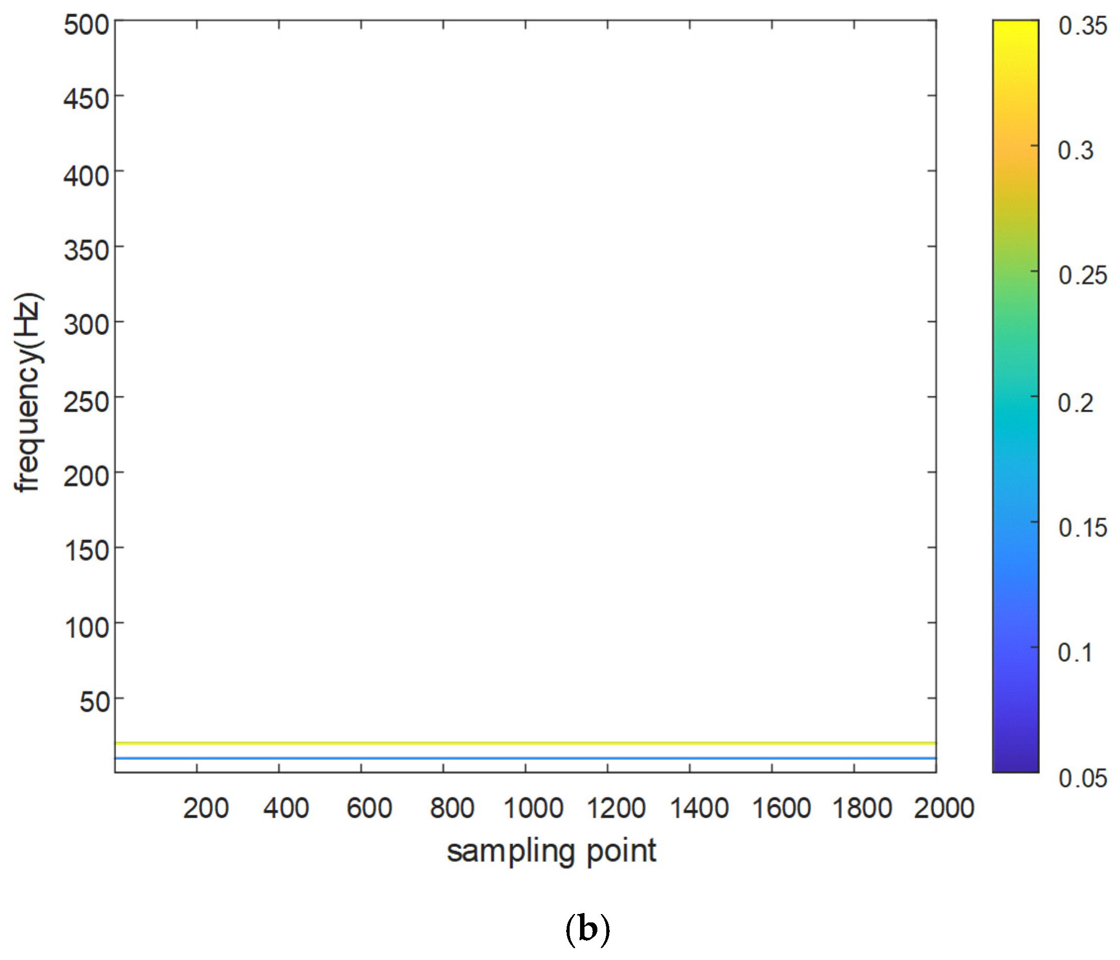
As an example, we shall illustrate the effects of SST on a composite signal
f(
t) consisting of two sinusoids. Assume that
f(
t) = cos(2π
f1t) + 2cos(2π
f2t + π/3), where
f1 and
f2, respectively, equal 10 and 20 Hz, and the sampling frequency is 1000 Hz. The reassigned TFR and its contour are shown in
Figure 1a,b, respectively, and the color bar relates to the absolute value of the TFR.
It can be seen that the sinusoids of f(t) are well-separated from each other and easily recognized. Intuitively, the enhanced TFR have “flat ridges” in the 3-D coordinate, or straight lines parallel to time axis in the 2-D coordinate. In fact, on the contour time-frequency plane, each of the parallel line corresponds to a unique IF value. The IF line can be seen as a unique characteristic and also the existing symbol for sinusoids.
3. Methodology for Sinusoidal Noise Removal
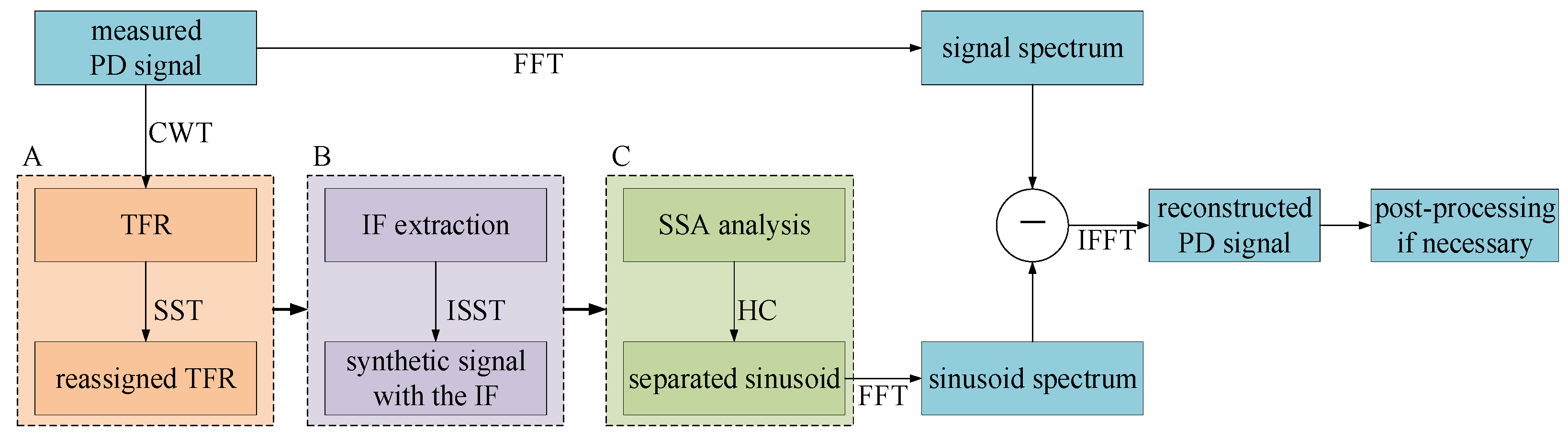
In order to remove sinusoidal noise from the measured PD signal, one possible way is to treat it as noise and suppress it as much as possible. However, taking into account that sinusoidal noise is deterministic, it can also be treated as the signal of interest from a different perspective, and some methods can be applied for their precise estimation and separation. Then, removal of the sinusoidal noise is achieved by simply subtracting it from the measured PD signal. Based on this idea, a method for sinusoidal noise removal is proposed below. The method consists of four parts, i.e., time–frequency analysis, IF recognition and the extraction of synthetic signals, SSA based separation of sinusoids, and, finally, the Fourier spectrum subtraction.
Since the IF of a sinusoid is identical to its own frequency, its energy concentrates on the specific IF line. Meanwhile, for nonsinusoidal signals such as the PD signal and white noise, their energy spread out on all or part of the time-frequency plane. As long as the sinusoid is dominant enough in measured PD, its specific IF line still remains recognizable with a small distortion.
Once the sinusoid is recognized, its IF line should be firstly extracted. Synthetic signal with the recognized IF is then recovered by inverse SST. The recovered synthetic signal keeps almost all the energy of the sinusoid and excludes most energy of other nonsinusoidal signals, which means the domination of the sinusoid. Therefore, the recovered signal can be decomposed as a sinusoid and the residue.
SSA can be applied for further separation. SVD is firstly applied to the Hankel matrix of the recovered synthetic signal, followed by HC to classify and assign the eigenvalues and vectors. After certain iterations, the sinusoid is finally reconstructed and extracted from the measured PD signal.
Although the extracted sinusoid can be directly subtracted from the measured PD signal in time domain, tiny errors may accumulate during the estimation procedures described above, thus leading to great distortions. In fact, a more robust way can be applied for sinusoid removal, i.e., the sinusoid is subtracted from the measured PD signal in the frequency domain instead of time domain through fast Fourier transform (FFT). The detailed flow chart of the proposed method is shown in
Figure 2. Dashed Block A is the time–frequency analysis procedure, which has been introduced in
Section 2. Block B and C will be explained in the following subsections.
3.1. IF Extraction and Synthetic Signal Recovery
As shown in
Section 2, once the IF lines of sinusoidal noise are visible, they can then be extracted. An analysis optimization method for ridge extraction has been proposed by Carmona et al. in [
34]. In this method, a trade-off is minimized between ridge values and the TFR absolute values. However, the regularization parameters are difficult to determine, and the solving is also very sophisticated. For simpler implementation, a dynamic programming method is presented in [
30,
35] for ridge extraction, and it is utilized in this paper. It is a forward/backward greedy algorithm, which aims to extract the ridges of the TFR absolute value. In the algorithm, a curve extraction process is performed for a single ridge; as for multiple ridges, the process is performed again on the remaining TFR after setting values of the extracted TFR ridges to zeros.
The curve extraction process is described as follows in detail: in the forward procedure, computation is operated on the minus logarithm of the normalized TFR absolute value, i.e., on
F = −ln(
E), where
E = |TFR|
2/sum(|TFR|
2). Minimization of
F is equivalent to the maximization of
E, and thus the maximization of |TFR|. In the computation progress, both values of
F and the penalty traversing across frequency bins are taken into consideration. For the (
i,
j) point of
F, its value is adjusted to the sum of its original value and the penalized minimum of the
i − 1 th time bin. The computation on each time bin of
F is operated from the first time bin to the next. In the backward searching procedure, the minimum of
F on the last time bin is firstly retrieved, and computation is operated from the last time bin to the previous. For the
i th time bin, the
j th frequency bin is recorded if the value of point (
i,
j) is closest to the minimum on the
i + 1 th time bin. The pseudo code of this algorithm is shown in Algorithm 1.
| Algorithm 1. Pseudo-code of ridge extraction algorithm. |
| Input: TFR, the penalty parameter λ, the threshold ε |
| ComputeM = number of TFR rows; N = number of TFR columns; E = |TFR|2/sum(|TFR|2), F = −ln(E) |
| %Forward Procedure |
| Fval ← zeros(M, N), For i = 1:M, Fval(i,1) ← F(i,1), end |
| Fori = 2:N |
| Forj = 1:M |
| Fork = 1:M, Fval(j, i) ← min[Fval(k, i − 1) + λ(k − j)2], end |
| Fval(j, i) ← Fval(j, i) + F(j, i) |
| end |
| end |
| %Backward Procedure |
| Freq ← zeros(1, N), Freq(N) ← argmin[Fval(:, N)], |
| Fori = N − 1:1 |
| val ← Fval(Freq(i + 1), i + 1)-F(Freq(i + 1), i + 1) |
| Forj = 1:M |
| If|val-Fval(j, i) − λ(Freq(i + 1) − j)2| < ε, Freq(i) = j, break, end |
| end |
| end |
| Output: Freq |
After extracting the IF of each sinusoid, inverse SST can be applied and the synthetic signals corresponding to each IF can be recovered then. In these signals, sinusoid dominates because it retains almost all its energy, while energies of other signals are greatly reduced.
3.2. SSA Analysis
For the synthetic signals obtained in the
Section 3.1, each of them can be regarded as a composite signal whose components have similar IF characteristics. As a consequence, they can not be distinguished directly in frequency domain. However, the components vary greatly from each other in waveform. By studying their different characteristics in the time domain, the real sinusoid can be approximately separated.
A powerful tool named SSA for signal analysis in time domain is proposed in [
32]. The underlying idea is that the Hankel matrix of composite signals is decomposed by SVD, and the components can be classified by different singular values. Indeed, HC is utilized such that the singular values can be assigned to predefined classes. The detailed procedure is described as follows for separation of sinusoid from the synthetic signal:
Firstly, for a length-N signal, its Hankel matrix X is constructed. The size of X is L × K, where K = N − L + 1, L is defined by the user and set smaller than K.
Secondly, SVD is applied to
X, and
X can be decomposed as the sum of
R independent matrices, as shown in Equation (16).
where
R is the rank of
X,
Σ = diag(
σ1...
σR), and each
σi is the
i th singular value.
U and
V are the eigen matrices whose
i th columns relate to
σi. Therefore, each eigen triple (
σi,
ui,
vi) of
Xi can be obtained.
Thirdly, HC is performed on the signals in time domain reconstructed by each
Xi. Before classification, each reconstructed
xi(
n) is obtained through diagonal averaging, as shown in Equation (17).
The classification procedure is initialized by assigning each
xi(
n) to a distinct class, and the minimal distance
d between two classes is computed by Equation (18).
where < > is the inner product of two vectors, and || ||is the two-norm operator of a vector.
Then, the classification procedure is iterated by merging the two nearest classes into a new class until the predefined number of classes is reached. Finally, the sinusoid is approximately separated from other signals.
3.3. Sinusoidal Noise Removal
In
Section 3.1 and
Section 3.2 above, it has been explained how to obtain the estimated sinusoids. Intuitively, directly subtracting the estimated sinusoids from the measured PD signal in time domain seems just enough. However, the estimated IF slightly differs from the real frequency of each sinusoid. Therefore,
a periodic oscillation error in the time domain exists owing to this slight difference. Meanwhile, the SSA procedure also brings inevitable errors. These errors will lead to great distortion. As an alternative, the Fourier spectrum subtraction based on FFT in the frequency domain is proposed. It will outperform the time domain subtraction and greatly reduce the errors.
The underlying reason behind the choice can be summarized as follows: firstly, the Fourier spectrum of each sinusoid around its estimated IF can be easily recognized; also, the slight difference between estimated IF and the real frequency may be cancelled due to the resolution; finally, FFT is perfectly invertible, which ensures the accurate reconstruction in time domain.
It is worth noting that the proposed method is only able to remove the sinusoidal noise. Therefore, white noise still exists after the removal. For further denoising, a classic method such as wavelet thresholding can be applied to refine the reconstructed PD signal.
4. Case Analysis of Sinusoidal Noise Removal in Noisy PD
In order to verify the effectiveness and robustness of the proposed method, a numerical simulation is carried out in this section. DEP and DOP signals are adopted to simulate the PD signal in this paper, as suggested in [
13]. The signals are, respectively, denoted as
s1 and
s2, where
s1 =
Ae−t/τ1sin(2
πf0t), and
s2 =
A(
e−t/τ1 −
e−t/τ2)sin(2
πf0t). In this section, three types of PD signals are directly obtained by assigning different parameters to
s1 and
s2. They are denoted as PD1 to PD3, respectively, with their parameters shown in
Table 1.
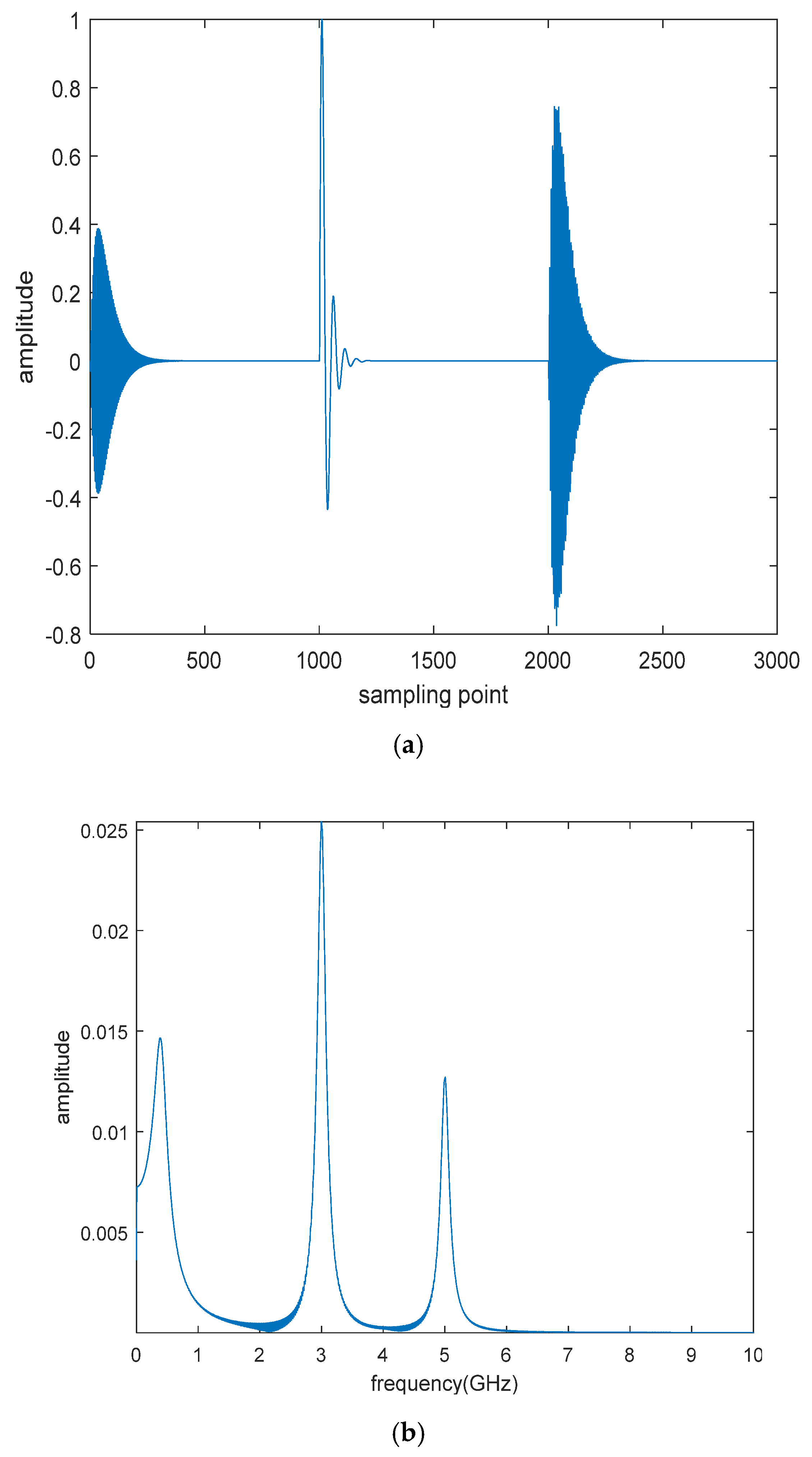
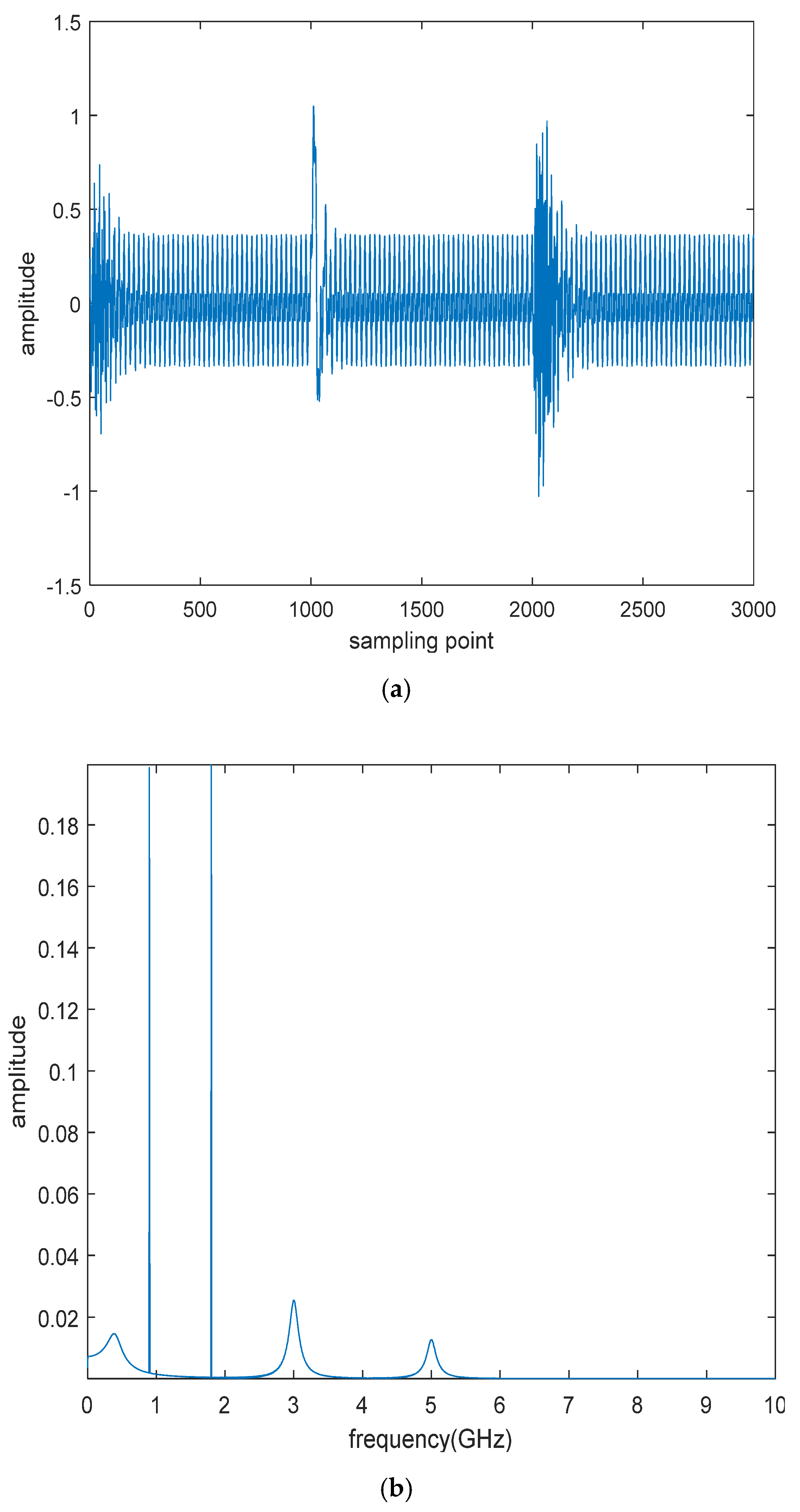
A more complex PD signal is then synthesized by the normalized combination of PD1 to PD3, i.e., PD = [PD3, PD1, PD2], and the peak amplitude of PD is normalized to be 1. Pure PD in time domain and frequency domain are shown in
Figure 3a,b.
There are two cases to be discussed here, i.e., (1) PD signal contaminated by sinusoidal noise only and (2) PD signal contaminated by both sinusoidal noise and white noise.
4.1. Case 1: Sinusoidal Noise Only
The sinusoidal noise
s(
t) is set to be a composite of two sinusoids, i.e.,
s(
t) = 0.2cos(2
πf1t +
π/3) + 0.2cos(2
πf2t +
π/4), where
f1 = 0.9 GHz and
f2 = 1.8 GHz, and its length is equal to that of PD. The noisy PD in time domain and in frequency domain are shown in
Figure 4a,b.
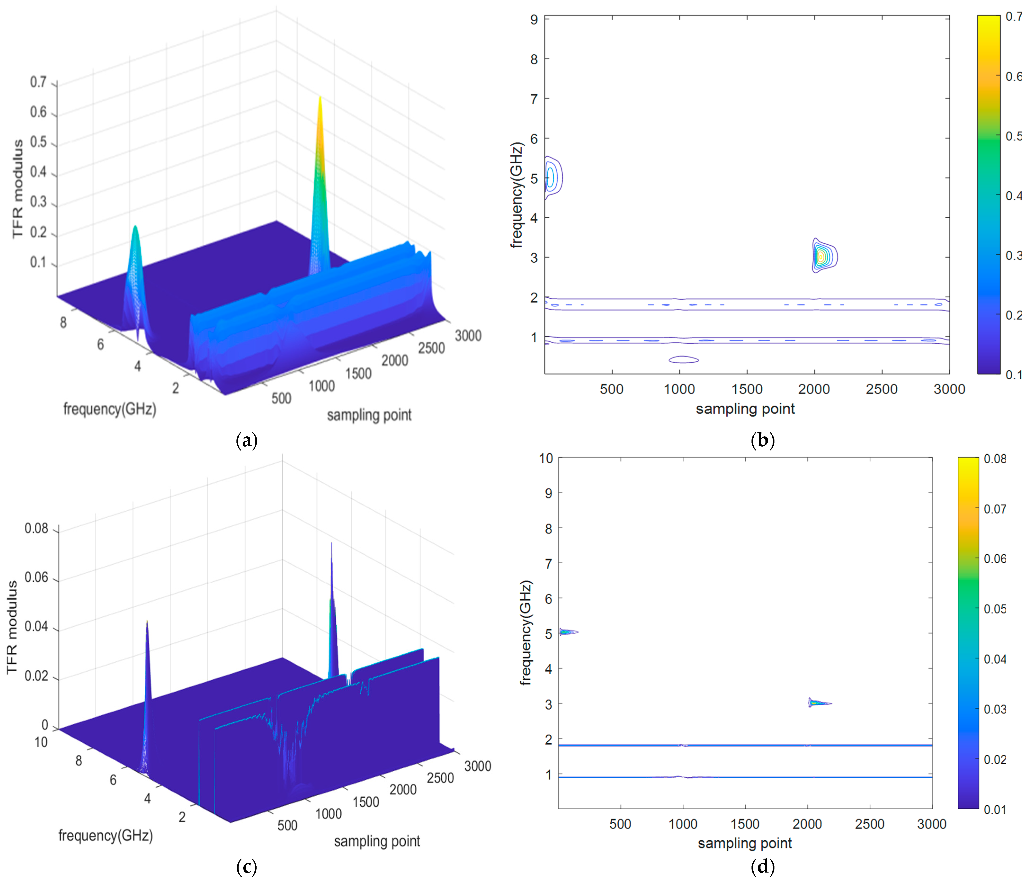
The CWT TFR and the reassigned TFR by SST are shown in
Figure 5, where the color bars relate to the absolute value of the TFR. It is clearly shown that CWT TFR is vague to analyze; meanwhile, the TFR is greatly enhanced by SST; thus, the IF lines of sinusoidal noise can be distinguished and then extracted. Two straight lines can be clearly recognized without uncertainty, which is inevitable in CWT.
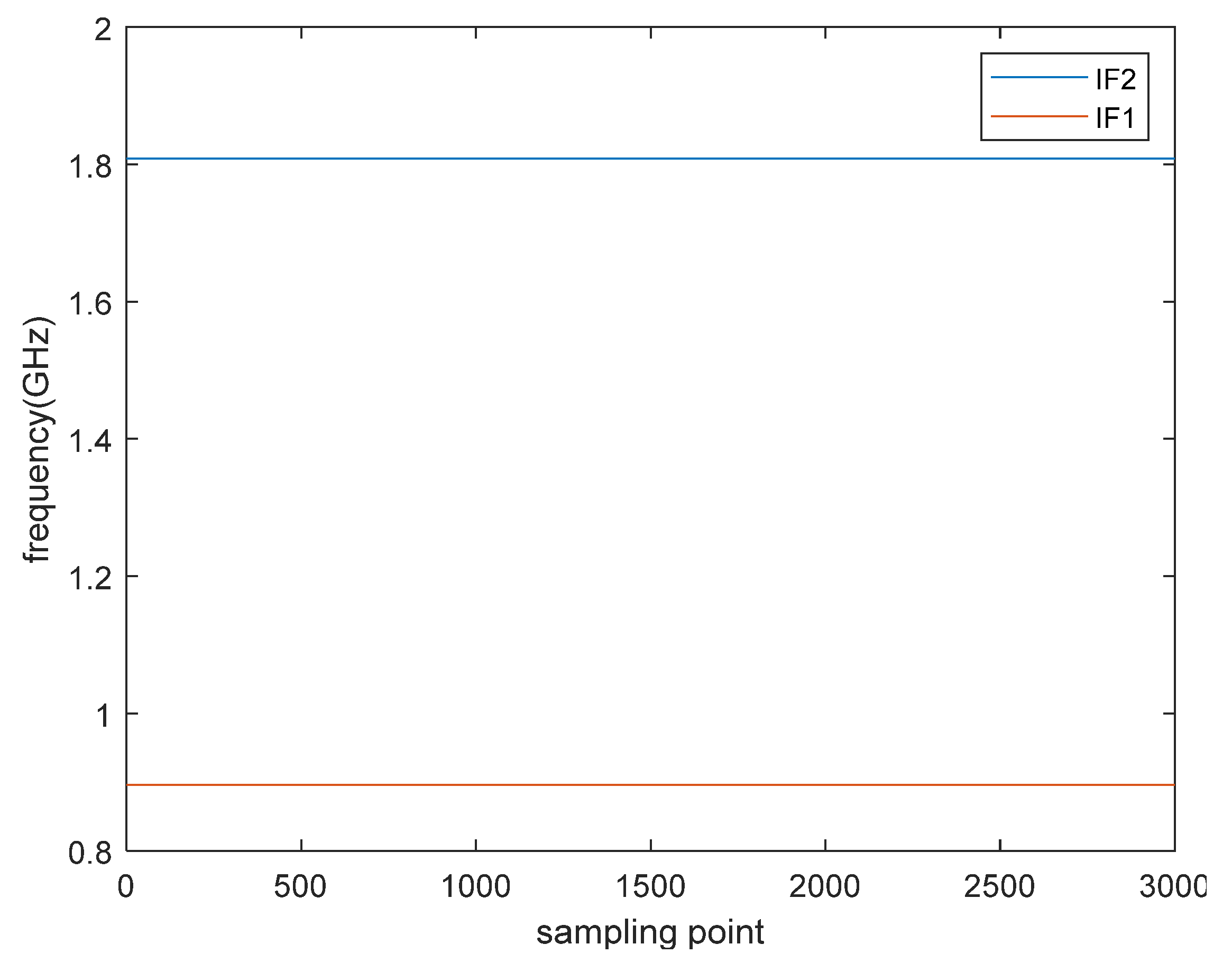
Due to the fact that IF lines of sinusoidal noise are known to be constant as a priori, a large
λ as well as a small threshold
ε shall be adopted to extract the value of the IF lines. In this paper, they are set to be 3000 and 10
−8, respectively. The extracted lines are shown in
Figure 6, and their values are, respectively, 0.8961 and 1.809 GHz. Obviously, the estimated frequencies are quite close to the real ones.
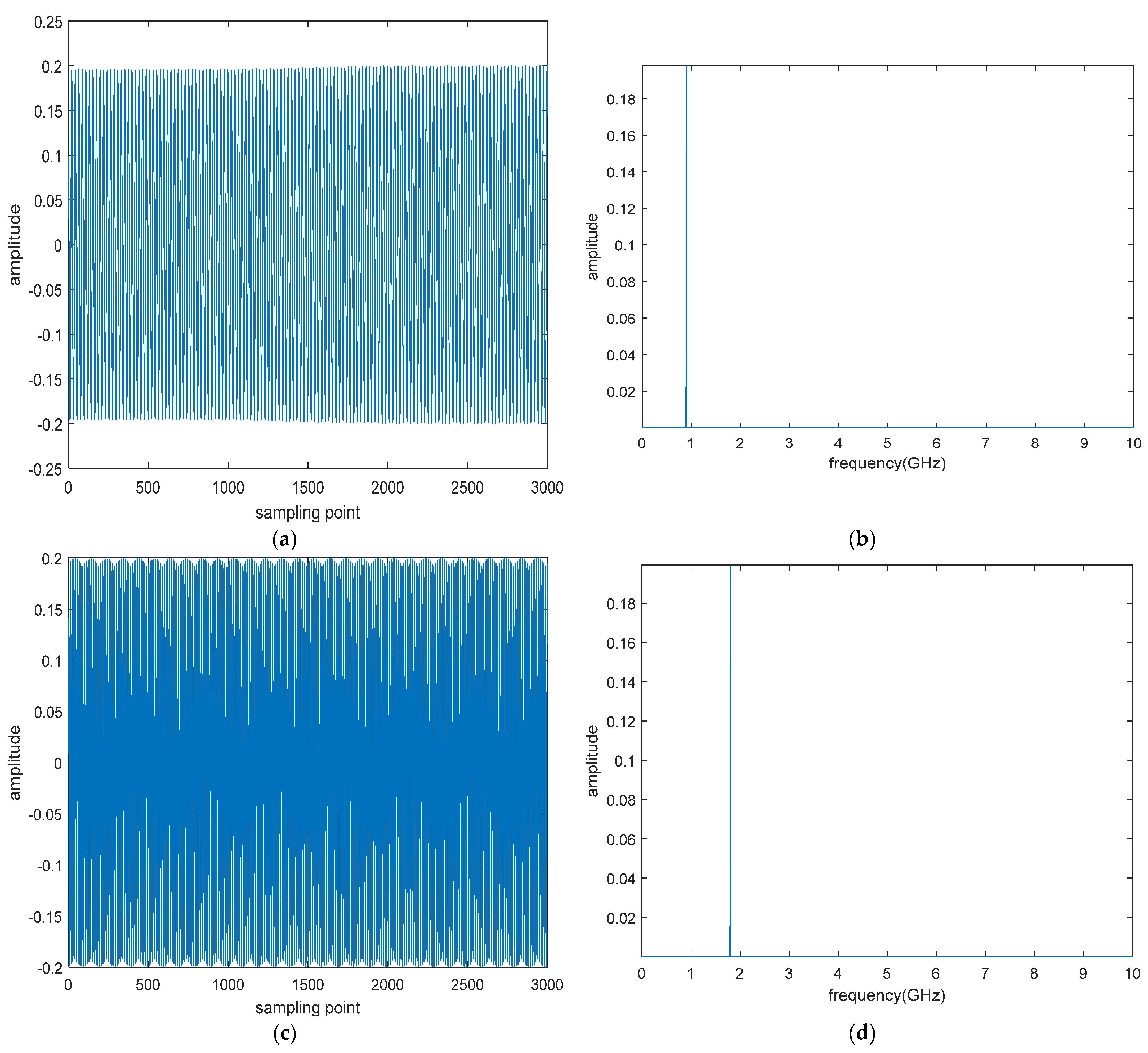
The synthetic signals are recovered from each IF by inverse SST, and they are consequently refined by SSA. The refined signals denoted as srec1 and srec2 as well as their Fourier spectrum are shown in
Figure 7. The estimated amplitude, phase, and frequency of each sinusoid are shown in
Table 2. By calculating the relative errors, it can be seen that estimated parameters are quite close to the real ones.
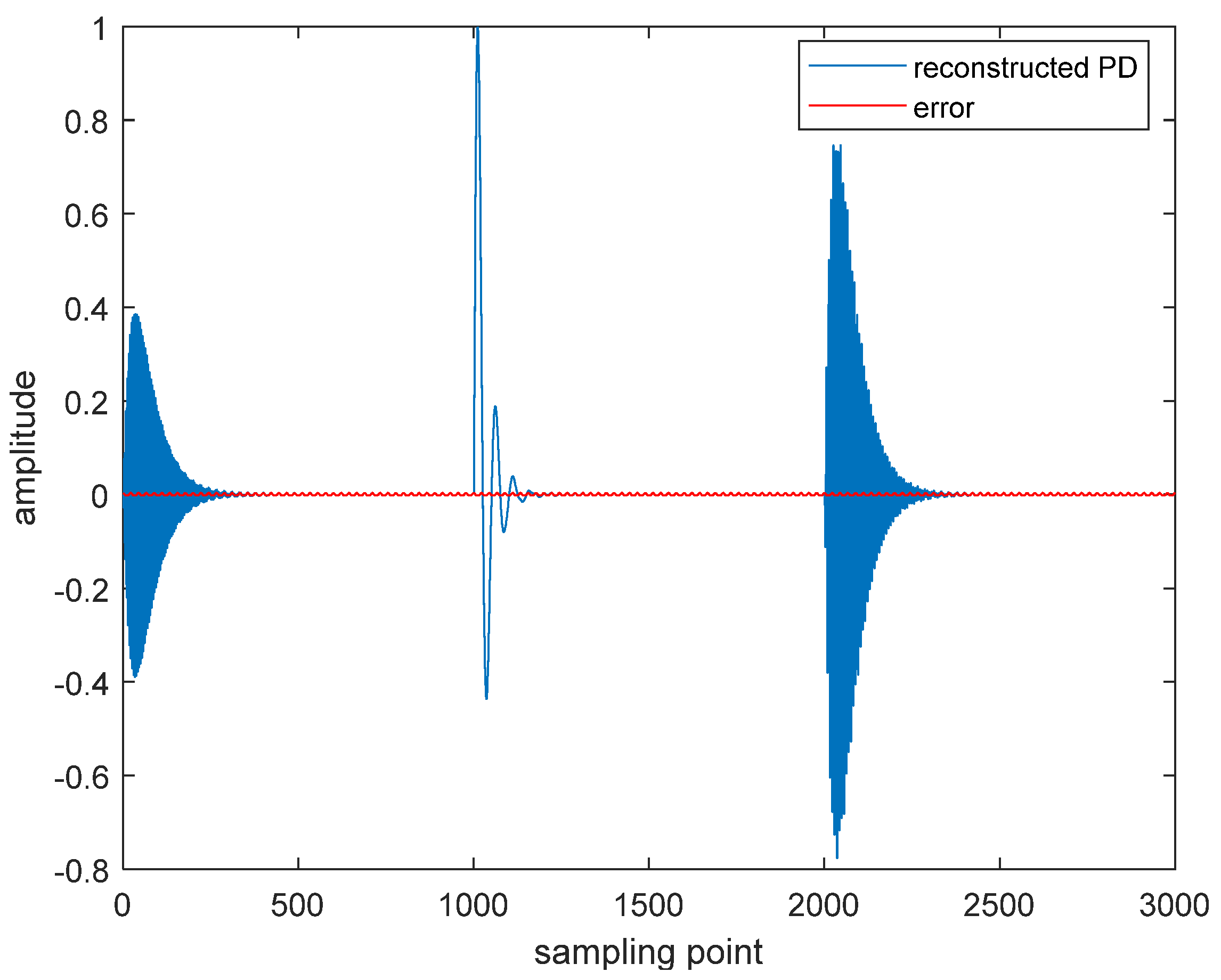
After removing the sinusoidal noise, the finally reconstructed PD signal is obtained. The reconstructed PD signal as well as the difference between it and pure PD signal is shown in
Figure 8. It can be seen that the reconstructed PD signal is almost equal to the pure PD, except for a negligible oscillation error.
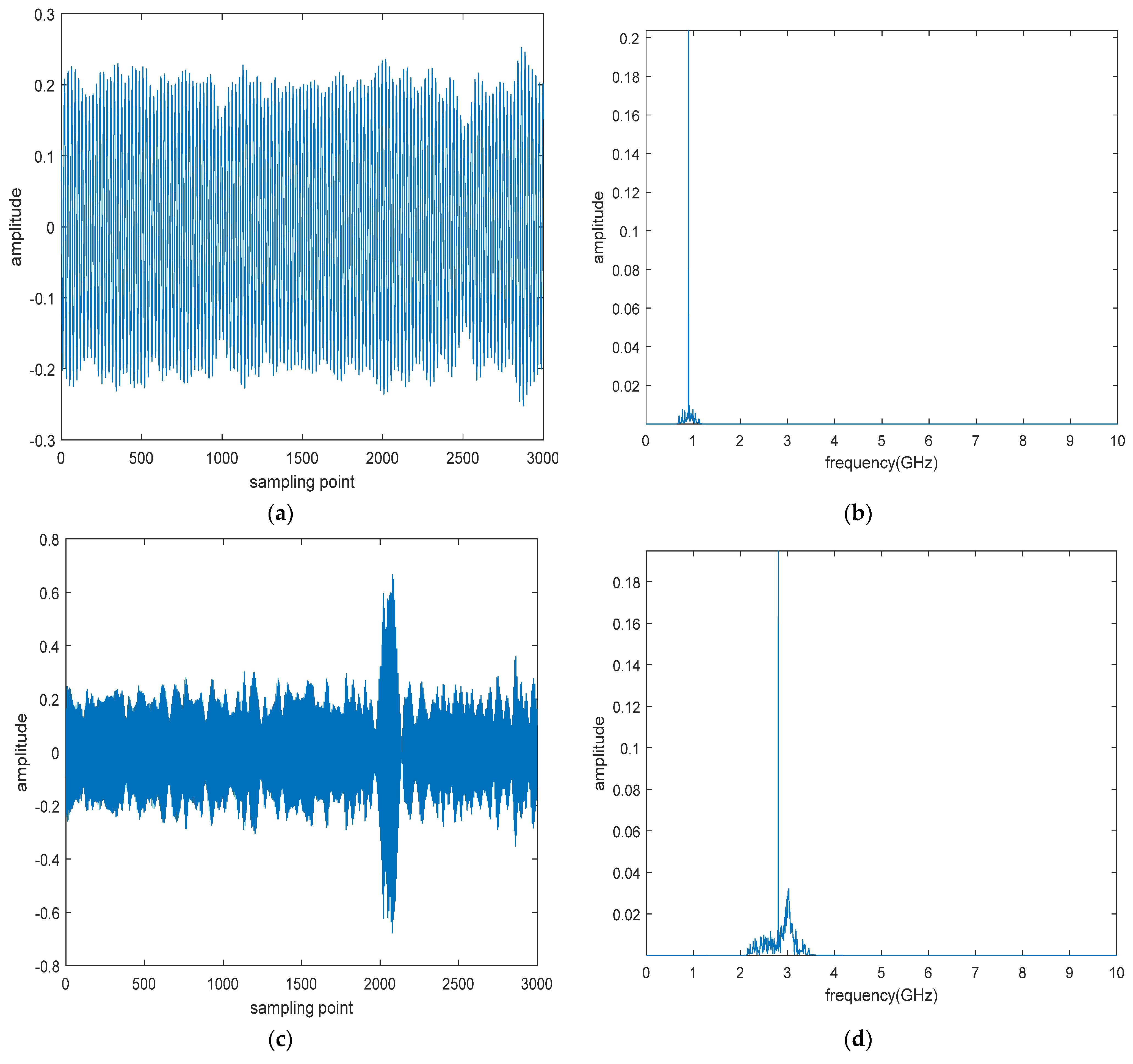
4.2. Case 2: Both Sinusoidal Noise and White Noise
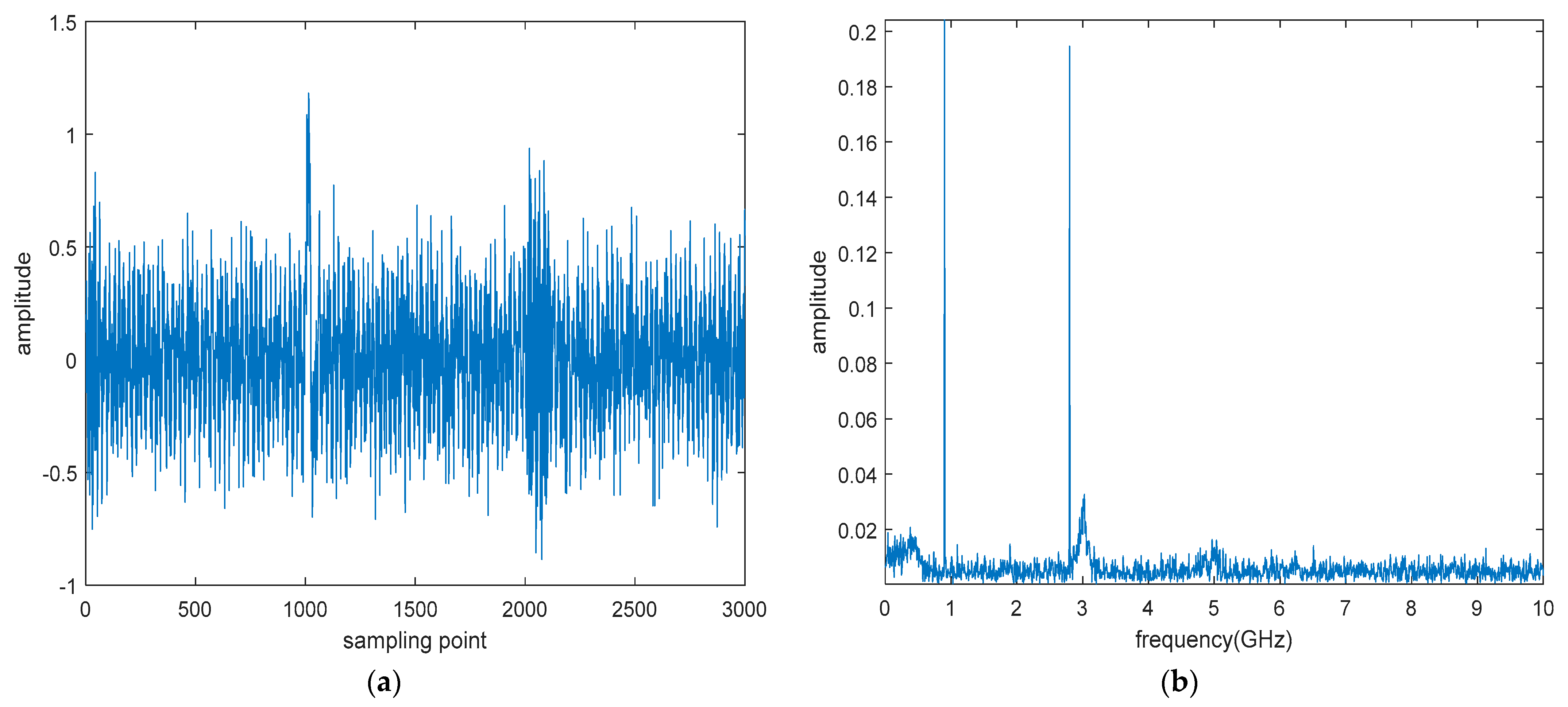
Although the proposed method works well to remove the sinusoidal noise from pure PD signal, white noise is not taken into consideration. The robustness of the method to white noise is validated here. The Gaussian white noise is firstly added to pure PD signal with the signal to noise ratio (SNR) set to be −2.2, and then the sinusoidal noise is also added. Additionally, in order to study the performance of the proposed method, we decide to set the frequency of one sinusoid closer to the band of frequencies corresponding to the pure PD. The sinusoidal noise
s(
t) is then set to be
s(
t) = 0.2cos(2
πf1t +
π/3) + 0.2cos(2
πf2t +
π/4), where
f1 = 0.9 GHz and
f2 = 2.8 GHz. The noisy PD and its spectrum in frequency domain are shown in
Figure 9. Similarly, steps in
Section 4.1 are performed once again for signal reconstruction.
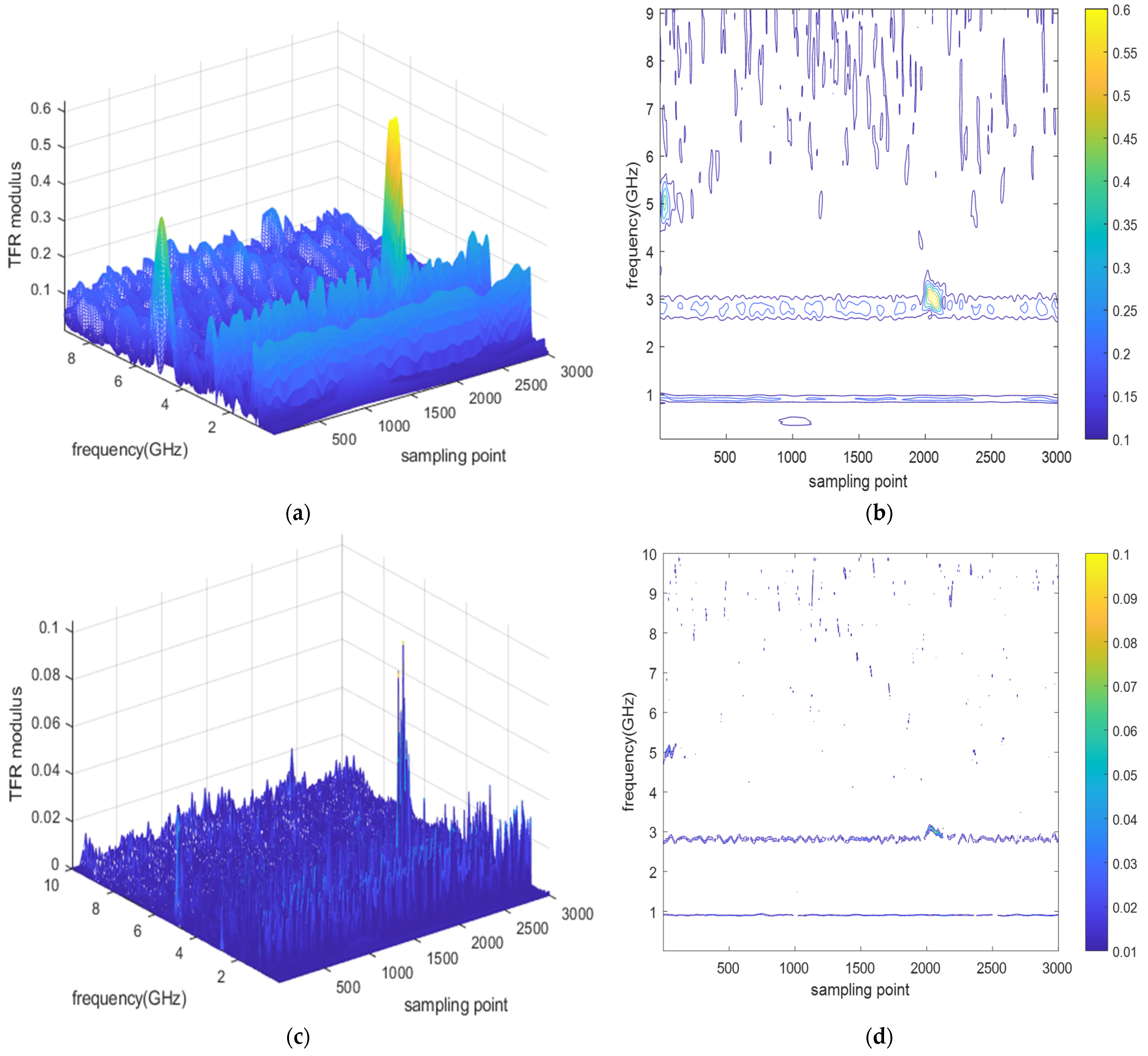
The CWT TFR and the reassigned TFR are shown in
Figure 10. Similar to the case mentioned in
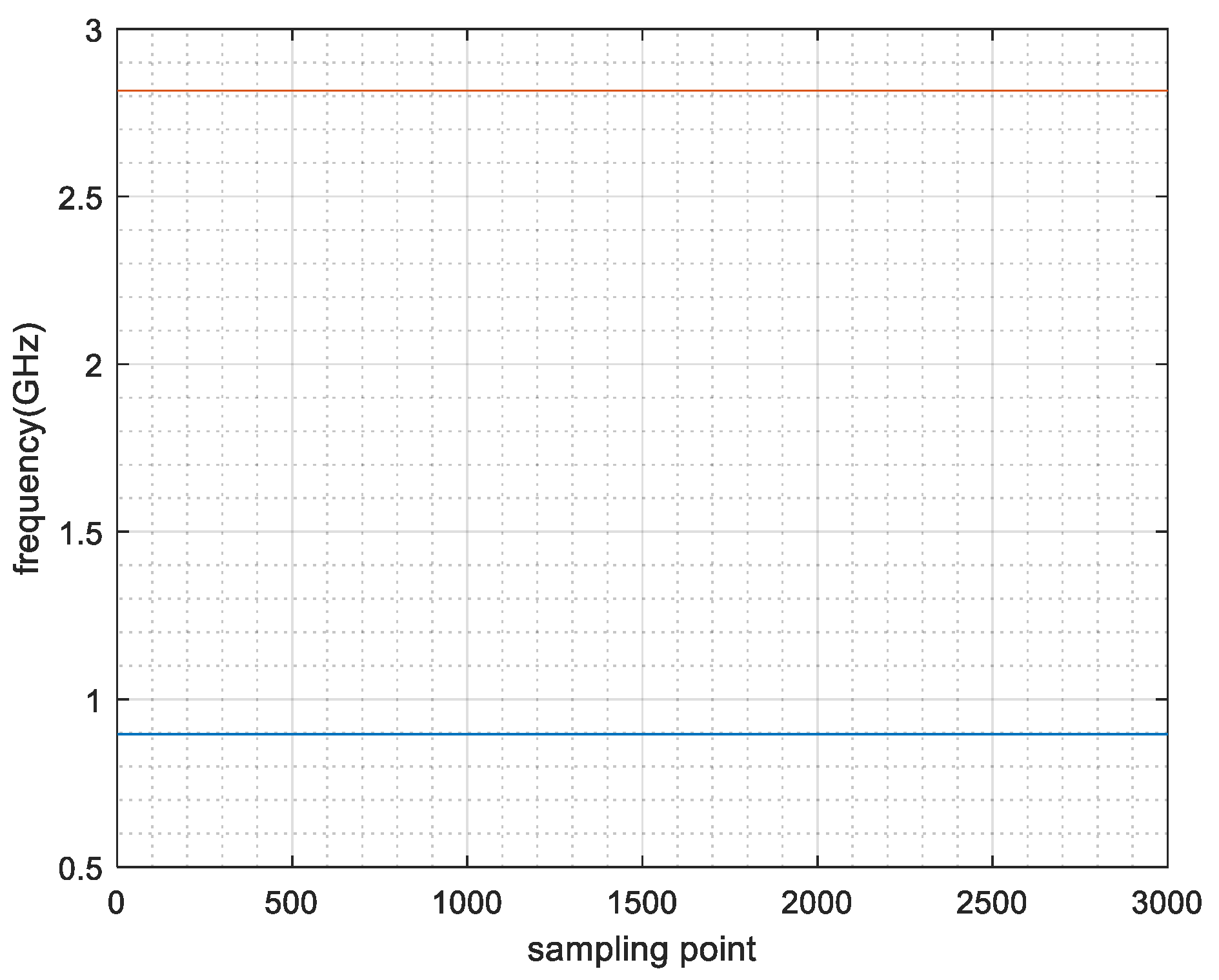
Section 4.1, the IF lines of sinusoidal noise can still be recognized and extracted, as shown in
Figure 11. The refined synthetic signal of each sinusoid and the spectrum in frequency domain are shown in
Figure 12.
The estimated amplitude, phase, and frequency of each sinusoid are also shown in
Table 3. The relative errors demonstrate the robustness of the proposed method to white noise.
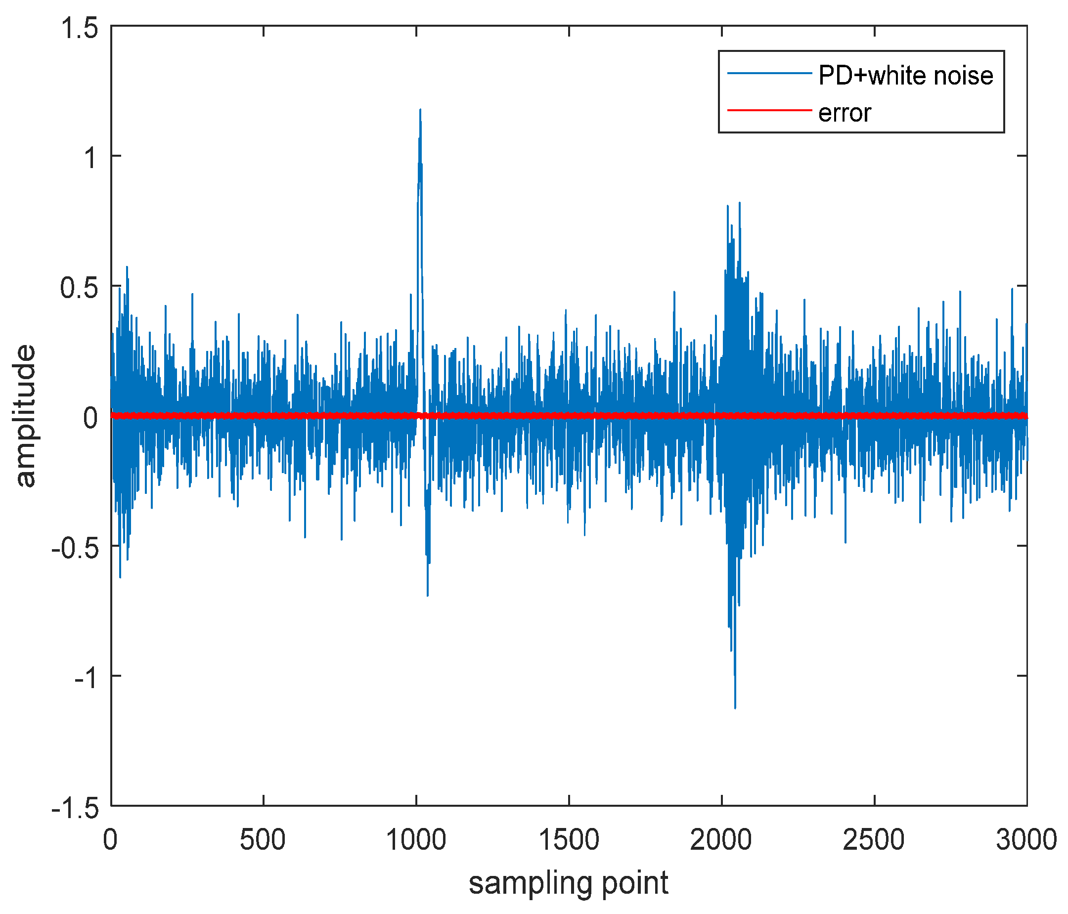
After Fourier spectrum subtraction, the sinusoidal noise is almost removed from the original noisy PD signal. Then, the processed PD signal is compared with the pure PD signal contaminated by white noise only. The pure PD signal contaminated by white noise only is shown in
Figure 13. Meanwhile, the difference between it and the processed PD signal is also shown. It can be seen that the proposed method still removes sinusoidal noise effectively, while hardly distorting the pure PD signal or the white noise.
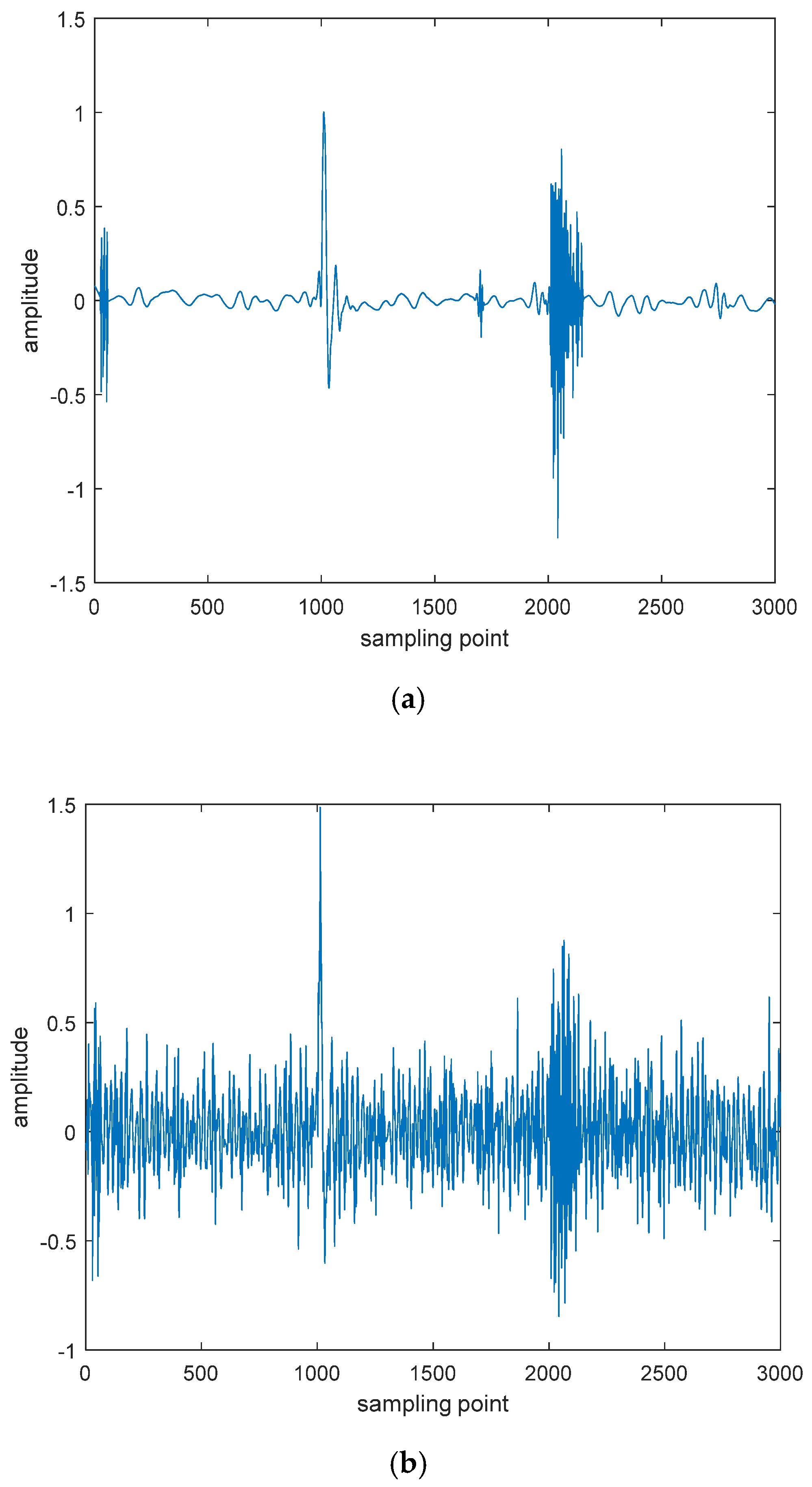
After the removal of sinusoidal noise, wavelet thresholding follows to suppress the white noise. In this paper, db6 wavelet, hard thresholding, and the Stein’s unbiased risk estimation (SURE) rule are selected. The decomposition level is set to be 5. The result is shown in
Figure 14a, and clearly both sinusoidal noise and white noise are well-reduced. As a comparison, traditional EMD is also applied to the original noisy PD signal. The result is shown in
Figure 14b, and intuitively, the proposed method performs much better.
In order to quantitatively evaluate the proposed method and EMD, three indexes are introduced here, i.e., SNR, mean square error (MSE), and normalized correlation coefficient (NCC) [
36]. Smaller MSE and greater SNR and NCC stand for better results. The computed results are shown in
Table 4. It can be seen that the proposed method obviously outperforms EMD, which is able to verify its effectiveness and robustness.
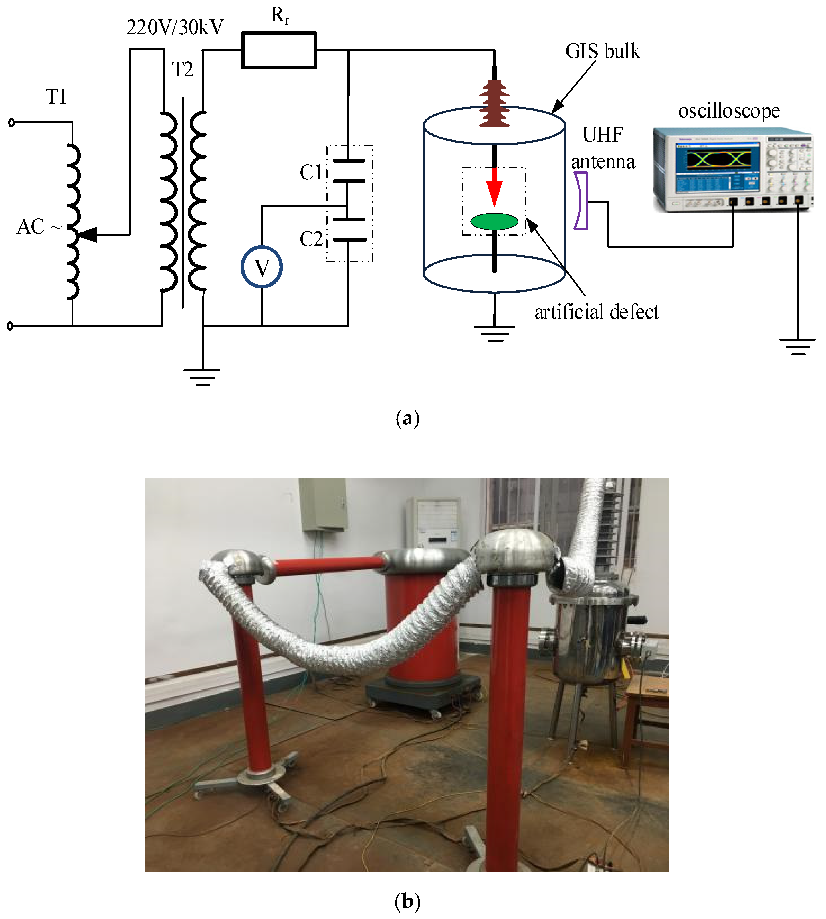
5. Experimental Case Analysis
In order to verify the effectiveness of the proposed method for real signals, the experimental platform is set up in laboratory for PD signal measurement. The experiment is conducted on gas-insulated switchgear (GIS) with sulfur hexafluoride (SF
6) as the medium and artificial defect to generate PD signal. The schematic diagram and measurement setup of the experiment are shown in
Figure 15.
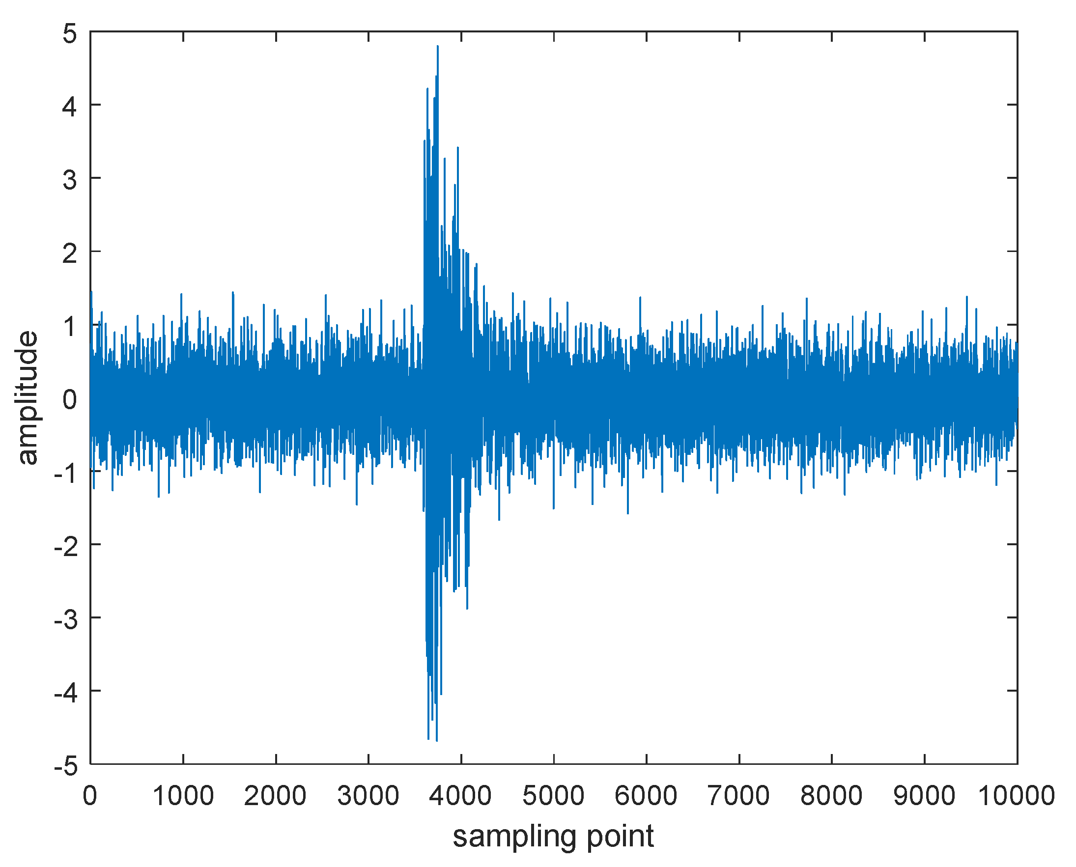
In the experiment, a power transformer with adjustable output voltage is used, and the needle-plane electrode is used as artificial defect. The generated PD signal will be able to propagate through the glass observation window and then be measured by the UHF antenna. The oscilloscope is Tektronix DPO7254C, and its sampling frequency is set to be 10 GHz. The measured PD signal with 10,000 sampling points is shown in
Figure 16, and the unit of its amplitude is mV.
Since the laboratory is away from interference sources of sinusoidal noise, artificial sinusoidal noise is added to the measured PD signal to verify the effectiveness of the proposed method in this paper, which is same as proposed in [
6,
11,
12]. The sinusoidal noise
s(
t) is then set to be
s(
t) = 1cos(2
πf1t +
π/5) + 1.5cos(2
πf2t +
π/4) + 0.5cos(2
πf2t +
π/3), where
f1 = 0.3 GHz,
f2 = 0.5 GHz, and
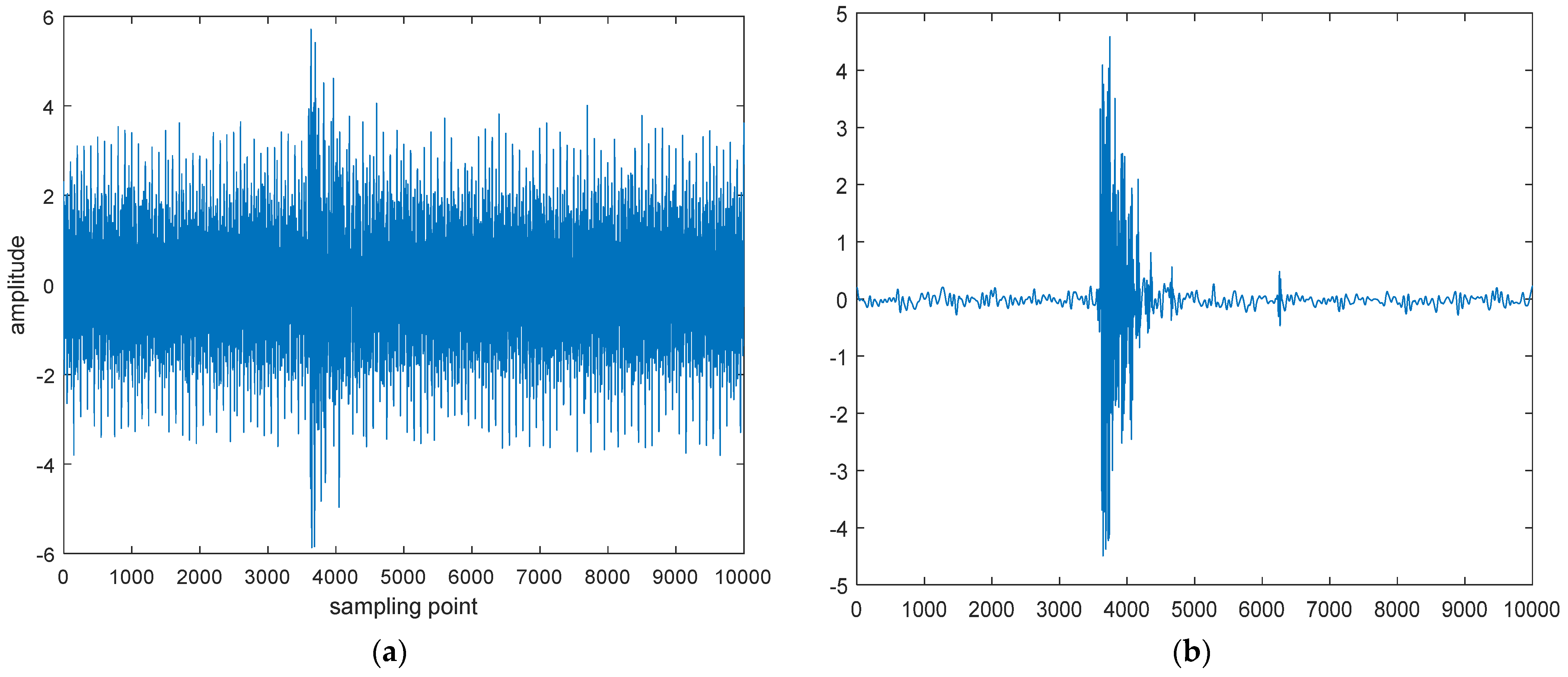
f3 = 0.9 GHz. The noisy PD signal as well as its processed version are shown in
Figure 17. It can be seen that, in the processed PD signal, sinusoidal noise has been effectively removed, which verifies that the proposed method also works for real-measured signal. However, it should be noted that if the frequencies of each sinusoid are too close to each other, the proposed method may not be able to identify each IF. Consequently, it will fail to remove the sinusoidal noise. Additionally, an oscilloscope with high-enough sampling frequency is necessary, usually up to 10 GHz.
6. Conclusions
In this paper, instantaneous frequency (IF) is introduced, and a new and effective method based on combination of SST and SSA is proposed for sinusoidal noise removal in PD signals.
SST is firstly used for IF recognition and ridge extraction, synthetic signals of the IFs are then recovered by inverse SST. Consequently, SSA is performed on the synthetic signals for further refinement, and, finally, Fourier spectrum subtraction removes the sinusoidal noise. Based on the numerical simulation, the following conclusions can be drawn:
- (1)
SST sharpens the TFR obtained by CWT and greatly reduces the uncertainty to recognize IF lines belonging to each sinusoid, even with smaller amplitudes than that of PD signal.
- (2)
The proposed method works well to remove the sinusoidal noise; meanwhile, it hardly distorts the waveform of other nonsinusoidal signals. Additionally, the proposed method is robust to white noise and outperforms traditional EMD method.
- (3)
As for further research, more complex noises may be taken into consideration, such as signals with transient frequencies.


