Article

A Deep Learning-Based Approach for Generation Expansion Planning Considering Power Plants Lifetime

by
Majid Dehghani
1,
Mohammad Taghipour
1,
Saleh Sadeghi Gougheri
2,
Amirhossein Nikoofard
2,
Gevork B. Gharehpetian
1 and
Mahdi Khosravy
3,*
1
Department of Electrical Engineering, Amirkabir University of Technology, Tehran 159163-4311, Iran
2
Department of Electrical Engineering, K. N. Toosi University of Technology, Tehran 196976-4499, Iran
3
Cross Labs, Cross-Compass Ltd., Tokyo 104-0045, Japan
*
Author to whom correspondence should be addressed.
Submission received: 22 October 2021 / Revised: 18 November 2021 / Accepted: 19 November 2021 / Published: 1 December 2021
(This article belongs to the Special Issue Power System Planning and Quality Control)

Abstract

:
In Generation Expansion Planning (GEP), the power plants lifetime is one of the most important factors which to the best knowledge of the authors, has not been investigated in the literature. In this article, the power plants lifetime effect on GEP is investigated. In addition, the deep learning-based approaches are widely used for time series forecasting. Therefore, a new version of Long short-term memory (LSTM) networks known as Bi-directional LSTM (BLSTM) networks are used in this paper to forecast annual peak load of the power system. For carbon emissions, the cost of carbon is considered as the penalty of pollution in the objective function. The proposed approach is evaluated by a test network and then applied to Iran power system as a large-scale grid. The simulations by GAMS (General Algebraic Modeling System, Washington, DC, USA) software show that due to consideration of lifetime as a constraint, the total cost of the GEP problem decreases by 5.28% and 7.9% for the test system and Iran power system, respectively.

1. Introduction

Nowadays, generation expansion planning (GEP) is an inevitable and important issue for power system planners due to energy consumption growth. In this problem, technology type, installation time, and location of new power plants are determined to supply the predicted load with appropriate reliability [1].
From mathematical modeling viewpoint, the generation expansion problem can have many constraints and variables. In addition, there are various objective functions such as minimizing generation planning cost [2], maximizing profit in the market [3], maximizing reliability [4,5], minimizing environmental pollution [6], and combination of mentioned objective functions. The problem constraints include load supply, transmission lines, and generators capacity [7], and in some cases, greenhouse gas generation, and also some uncertainties [8,9] have been considered as constraint.
The authors of [10] have analyzed the GEP and the transmission expansion planning (TEP) of a large-scale network with renewable energy. The objective function is to minimize investment, maintenance, and fuel costs using a multi-cut Benders decomposition algorithm for the optimization. A comprehensive and accurate optimization model of China GEP has been presented in [11] and different types of power plants have been used. In [12], the effects of solar and wind power plant uncertainty on the GEP model of IEEE 300-bus have been investigated. In [13], the GEP problem has been modeled based on the game theory. The purpose of this article is to reduce carbon emissions by applying carbon taxes. In [14], a comprehensive and deep review has been performed about the GEP problems such as uncertainties, energy policies, low carbon economy requirements, renewable sources, electricity market, demand-side programs, distributed generation, and so on. A review of the GEP problems, which include renewable energy power plants, has been carried out in [15,16] and the operational flexibility issues have been investigated and several ways have been proposed for solving this challenge. In [17], a review has been performed about adding renewable power plants to the GEP model and three issues of optimization models, general/partial equilibrium models, and alternative models, have been studied. All the advantages and disadvantages of each model have been reviewed which has led to better perception of the expected results. In [18], the GEP mathematical modelling has been presented and pollutants and renewable energy effects have been investigated. In the article, 100 MW wind power plants have been used as candidate and shown that three 100 MW power plants in 14-years planning can be used. In [19], the wind power plant has been evaluated as a large portion of power generation and uncertainty effect of wind speed and gas power plants fuel price have been investigated. In [20], renewable energies have been used to minimize fuel cost and CO2 emission.
The GEP studies are based on the determination of annual peak load. Modeling the annual peak load uncertainty increases the accuracy of the results. Existing articles in the field of GEP, modelling the peak load uncertainty, can be divided into three categories. In the first category [2,4,6,18,21], the researchers have not considered the load uncertainty and only a standard load profile of [22] has been used. In the second category [1,3,7,8,19,23,24,25,26,27,28,29], the uncertainty of the load has been modelled using the annual load growth rate during the following years. In the third group of the research [30,31,32], the load uncertainty has been considered using different methods. The authors of [30] and [31] have used scenario-based methods and in [32], regression analysis has been used for forecasting the load. To have a good performance, scenario-based methods require the production of a large number of scenarios, which have high computational costs and are inefficient in large-scale problems [33]. In recent years, deep learning-based methods extensively have been used for modeling uncertainties in power systems [33,34]. Long short-term memory (LSTM) networks, which are a new version of recurrent neural networks (RNN), show good performance in modeling uncertainties such as short-term load forecasting [35], and electric vehicle demand modeling [36]. In the previous works, the deep-learning-based methods have not been used for forecasting the annual peak load.
The GEP optimal solution with carbon emission cost has been considered by many authors [37,38]. Currently, low-carbon technology is divided into two categories. In the first category, carbon is absorbed directly by some technologies such as carbon capture. In the second category, carbon emissions are reduced by using renewable energy instead of fossil fuel power plants or improving the efficiency of power plants [39]. The authors of [40] have presented an integrated generation and transmission expansion planning model with carbon capture systems. In this paper, the total cost including investment, generation, and carbon emission costs. In [41] a multi-period low carbon Generation Expansion Planning (LC-GEP) model is proposed under a low carbon policy. To obtain the optimal generation mix, a mixed-integer programming (MIP) model has been used under different carbon policies. In [42] a linear programming model for coordinated GEP and TEP is presented. Furthermore, the effects of different carbon emission policies on system planning have been considered.
According to the previous works that are reviewed in Table 1, the knowledge gap in this field can be defined as follows:
  • Investigating the effects of power plants’ lifetime constrain on new and existing plants. This constraint affects the GEP problem due to two practical reasons: 1-Some power plants have less lifetime than the planning horizon. This fact may increase the costs, and the GEP might have more cost than the case with a longer lifetime. 2-Some power plants may have derated efficiency due to aging, or out of date technologies in comparison with newer ones with less fuel consumption. Therefore, they should be replaced by new ones.
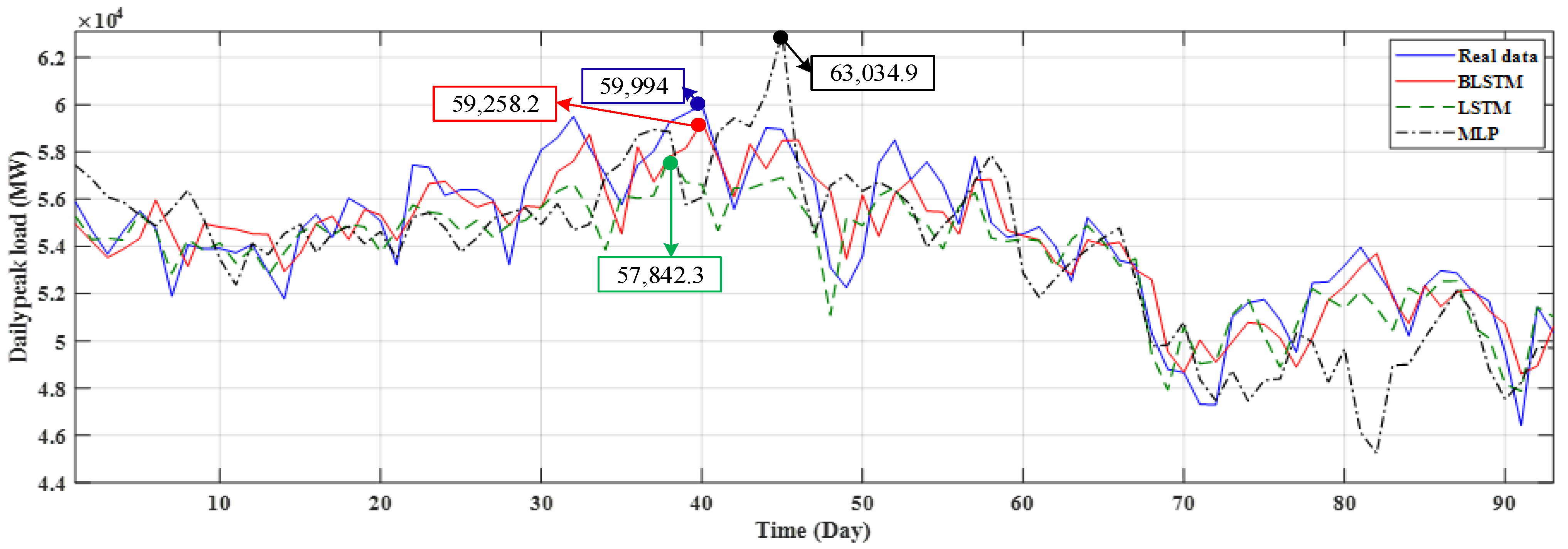
  • Using a new version of LSTM networks known as Bi-directional LSTM (BLSTM) networks for forecasting the annual peak load. The advantages of BLSTM networks compared to LSTM networks are its two feedforward and feedback loops, which lead to the use of the whole temporal horizon. This feature of BLSTM networks can increase accuracy in time series forecasting tasks.
  • Considering the carbon tax policy as a carbon emission reduction method in order to prevent the release of carbon into the environment
Some power plants go out of operation every year due to reaching the end-of-life. This issue is considered as a constraint in the model and a salvage value in the objective function. In addition, in the constraint of load and supply balance, the amount of load is equal to the output of the forecasted method (BLSTM networks). Considering carbon emissions will have a cost added to the objective function. As the objective function is minimized the carbon emissions will be reduced.
Table 1. Comparison between different works in the GEP.
Ref.GEPLifetime of Candidate PlantsLifetime of Existing PlantsLoad ForecastingCarbon EmissionRenewable Energy
[11]
[14]
[25]
[26]
[27]
[29]
[38]
[39]
[40]
This paper
The rest of this paper is organized as follows. The GEP model is introduced in Section 2. Section 3 describes the deep learning-based approach to forecast annual peak load. The simulation results are included in Section 4 followed by a conclusion in Section 5.

2. Objective Function

2.1. Investment, Operation, and Maintenance Cost

The purpose of the proposed model is to minimize the total cost of investment and operation costs. The objective function comprised of three terms: 1—investment cost 2—operation and maintenance cost and 3—salvage value which is shown in Equation (1).
M i n   t = 1 T { f t 1 ( U t ) + f t 2 ( X t ) f t 3 ( L t ) }
Subject to,
X t = X t 1 + U t L t ( t = 1 , , T )
The state equation for the dynamic planning problem is presented in Equation (2). The number of power plants per year is equal to the number of power plants of the previous year plus new power plants minus retired power plants.

2.2. Carbon Emission Cost

In this paper, the carbon tax policy as a carbon emission reduction method has been utilized in order to prevent the release of carbon into the environment. This tax is applied to fossil fuel power plants. It is necessary to add this cost to the objective function. Therefore, the objective function is proposed as follows:
M i n   t = 1 T { f t 1 ( U t ) + f t 2 ( X t ) + f t 3 ( X t ) f t 3 ( L t ) }

2.3. Constraints

In order to achieve an optimal expansion plan, several constraints such as lifetime, reserve margin, the maximum number of new plants, mix capacity, and loss of load probability (LOLP) constraints have been considered.

2.3.1. The Lifetime Constraint

In this paper, the impact of the lifetime constraint on new power plants as well as existing power plants has been investigated. When lifetime ends, that capacity will be out of the network. This is modeled as:
L i L i ¯ ( t = 1 , , T   and   j = 1 , , J )

2.3.2. The Reserve Margin Constraint

To achieve a stable operating point of the power system, the installed capacity has to be greater than the annual peak load of each year. The reserve margin constraint is given in Equation (5).
R _ R ( X t ) R ¯ ( t = 1 , , T )
The upper limits of the reserve margin is considered 60%, and the lower limits of it is 15%.

2.3.3. Maximum Number of New Plants Constraint

There are restrictions on the construction of various types of power plants. The number of new power plants in each year cannot exceed U ¯ t . This constraint is modeled as the following equation.
0 U t U ¯ t ( t = 1 , , T )

2.3.4. Mix Capacity Constraint

This constraint indicates the percentage of capacity of each power plant.
M _ t j i Ω j x t i M ¯ t j ( t = 1 , , T   and   j = 1 , , J )
The lower and upper bounds of the capacity mix are considered 0% to 30% for oil-fired, 0% to 40% for liquefied natural gas-fired (LNG-fired), 20% to 60% for coal-fired, and 30% to 60% for nuclear units.

2.3.5. The LOLP Constraint

This article is considered the LOLP. The LOLP measures a probability of outages to overall resource adequacy. The maximum amount of LOLP can be formulated as follows:
L O L P ( X t ) ε ( t = 1 , , T )

3. Deep Learning-Based Approach for Annual Peak Load Forecasting

In this section, LSTM networks are introduced first, and then BLSTM networks are described. Against standard feedforward neural networks, RNNs, which benefit from recurrent weights, can learn the temporal dependence among data. This property of RNNs has a significant effect on the accuracy of time series forecasting results [43]. The main challenges in the training of deep RNNs are vanishing and exploding gradients. To solve these problems, the robust version of RNNs known as LSTM networks have been introduced in [
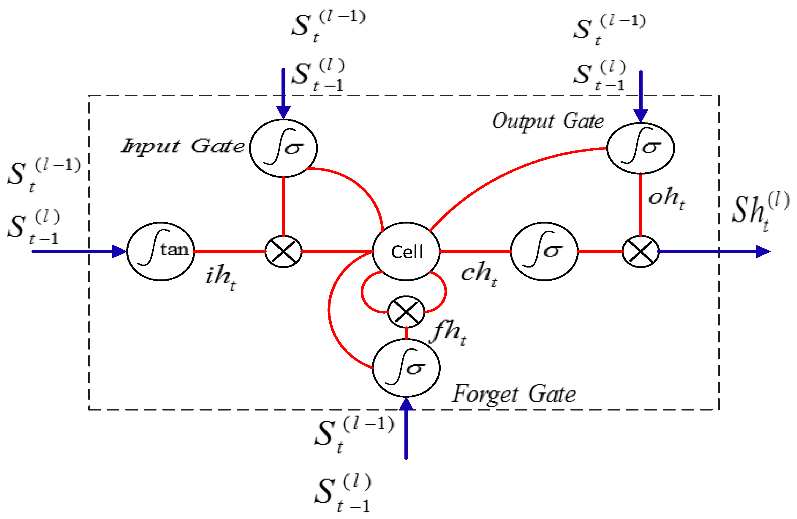
33]. The construction of an LSTM block is shown in Figure 1. Equations (9)–(13) describe the general formulation of an LSTM block [33,44]. In Equations (9), (10) and (12), the amount of outputs for input (it), forget (ft), and output (ot) gates are calculated, respectively. In addition, Equation (11) shows the cell state, and St is the output of LSTM block.:
i t = σ ( W i S t ( l 1 ) ) + W h i S ( t 1 ) + b i
f t = σ ( W i φ S t ( l 1 ) ) + W h φ S ( t 1 ) + b f
c t = f t c ( t 1 ) + i t t a n h ( W i γ S t ( l 1 ) + W h γ S ( t 1 ) + b c )
o t = σ ( W i o S t ( l 1 ) ) + W h o S ( t 1 ) + b o )
S t = o t t a n h ( c t )
where LSTM block variables are ( W i   , W i φ   , W i γ   ) ϵ r × n h   , ( W h i   , W h φ   , W h γ   ) ϵ n h × n h ,   ( b i   ,   b f   ,   b c   , b o   ) ϵ 1 × n h .
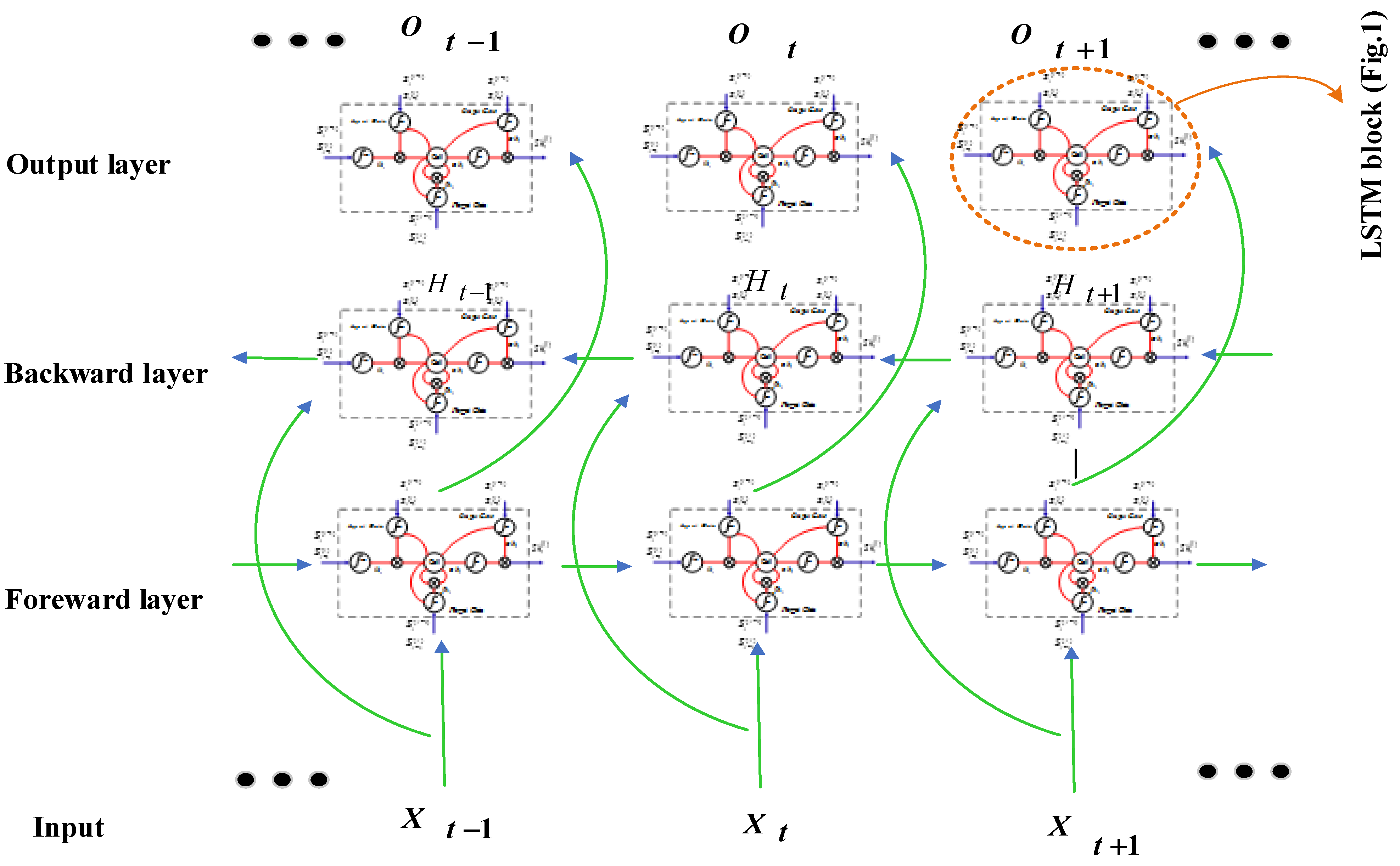
Figure 2 presents the structure of the BLSTM networks which models the long-term dependencies. The accuracy of time series forecasting results can be improved by considering the whole temporal horizon with two-directional memory of the BLSTM networks [45,46].
In the BLSTM networks, we have two groups of LSTM blocks, one as a backward layer and another as a forward layer, which provide two ways for transferring information; one from future to past and another way from past to future. As a result, BLSTM networks have high ability in feature extraction and good performance in time series forecasting for long term horizon.
The BLSTM is an appropriate solution, where we are facing with data whose outputs are employed as the input data in the future steps. This configuration brings a strong memory for the BLSTM network to remember and utilize all the useful previous and future features with high accuracy [47]. In the BLSTM networks, X t ϵ n × r is the mini-batch input data in a time step t, H t ϵ n × nh and H t ϵ n × nh are forward and backward hidden states which calculated based on Equations (14) and (15), respectively. Hidden state in a time step t is H t ϵ n × 2 nh , and output is O f n   ϵ n × no   which is calculated based on Equation (16).
  H t = t a n h ( X t W x h ( f ) + H t 1 ) W h h ( f ) + b h ( f )
H t = t a n h ( X t W x h ( b ) + H t 1 ) W h h ( b ) + b h ( b )  
O f n   = H t W o + b o  
BLSTM network variables are W x h   ( f ) ϵ r × n h , W h h   ( f ) ϵ n h × n h , b h   ( f ) ϵ r × n h , W x h   ( b ) ϵ r × n h , W h h   ( b ) ϵ n h × n h , and b h   ( b ) ϵ 1 × n h .

4. Case Studies

In this section, the effects of various power plants lifetime on a test system [22] and Iran large-scale power system [48] are investigated for a 30-year horizon using simulations.

4.1. Case 1: Test System

This system has 12 power plants that their data are given in Table 2. In this table, LNG and PWR (power plants) stand for liquefied natural gas and pressurized water reactor, receptively. Table 3 lists the forecasted peak demand for each year. Technical and economic data of candidate plants are presented in Table 4, where PHWR stands for pressurized heavy-water reactor. The planning horizon is divided into fifteen 2-year stages. To begin the simulation, the remaining lifetime of existing power plants are assumed as listed in Table 5.
Figure 3, Figure 4, Figure 5, Figure 6 and Figure 7 show the number of different power plants of the test system in a 30-year horizon. It can be seen that due to retirement, some power plants are out of plan in some years, but it is not efficient to rebuild these power plants and the remaining demand is supplied by constructing other power plants type. Figure 3 shows that the LNG power plants have been used at the end of the planning period more. Due to lower operating cost of coal power plants than the LNG type, these power plants have been used more throughout the period as shown in Figure 4. In Figure 5, two oil-fired power plants constructed in the 4th year are retired in the 22nd year. In this year, instead of constructing new oil-fired power plant, four new LNG power plants are built to provide load and supply balance. As shown in Figure 6 and Figure 7, due to the high investment cost and low operating cost of nuclear power plants, they have been used at the beginning of the period. Without considering the lifetime, it is necessary to rebuild the power plant(s) of the same type after retirement. Then, the GEP problem solving without considering the lifetime has more limitations. Therefore, the optimal result of the GEP problem considering the lifetime is always equal to or less than the optimal result of the same problem without considering lifetime.
Table 6 presents retired and new power plants of the test system in a 30-year horizon. It can be observed that the power plants are out of the plan when their lifetime spans. For instance, since oil-fired power plants lifetime is 20 years, two oil-fired power plants constructed in the 4th year are retired in the 22nd year. The red (blue) numbers indicate the conditions that the number of power plants constructed from a type is greater (less) than the number of retired power plants of the same type. According to Table 6, in the 26th year, two PWR power plants are retired and a new PWR power plant is rebuilt. Therefore, the total number of PWR power plants is decreased. This result is indicated in the 26th year of Figure 7, where the trend curve is decreasing. If the lifetime constraint is not considered, the total number of power plants is always increasing.
The total operation cost is obtained by the summation of all the years operation cost. The cost of the construction is only calculated in the year of power plant installation. Figure 8, Figure 9, Figure 10, Figure 11 and Figure 12 present a new and retired power plant capacity of each year. It can be observed that although PHWR and PWR power plants have high construction cost (Table 4), the low cost of the operation causes that a large share of the production is provided by PHWR and PWR plants in the early years of planning. On the contrary, according to Table 4, the least construction and the most operation cost belong to LNG power plants. Therefore, due to high operation cost, only one LNG power plant is constructed before the 16th year as shown in Figure 8.
The total cost with and without considering the lifetime for the test system is listed in Table 7. As can be seen, the total cost considering the lifetime constraint is improved by 5.28% in comparison with the total cost without considering the lifetime constraint.

4.2. Forecasting Annual Peak Load

The case study for forecasting annual peak load is the Iran network. Since there are not enough yearly peak load data for the training procedure of deep BLSTM network, July to September daily peak load data of Iran network are used in 10 years (2011–2020). The reason for using the daily peak load data from July to September is that the annual peak load of Iran network occurs in one of these three months. The dataset includes 930 data. In this case, 80%, 10%, and 10% of the dataset are allocated for the training, validation, and testing task, respectively. For forecasting the peak load of every day, 31 prior daily peak load data (31 × 1) are used. At the end of the forecasting procedure, the maximum value forecasted for July to September in a year is chosen as the peak load of that year. To show the performance of the BLSTM network, the year 2020 is selected as a test year. For the BLSTM network, 20 hidden layers are considered for each LSTM block, and the maximum number of epochs is set as 1000. The training procedure of the BLSTM network for annual peak load forecasting is carried out in Python using the “Keras” library.
To demonstrate the BLSTM performance, the BLSTM network results are compared with two other benchmark methods, i.e., the LSTM network and multi-layer perceptron (MLP). The forecasted results from July to September 2020 are presented in Figure 13.
To show the robustness of the BLSTM network, three error criteria of the forecasted results are calculated for different methods which are presented in Table 8. These error criteria are the mean absolute error (MAE), the mean absolute percentage error (MAPE), and the root mean square error (RMSE) [35]. As presented in Table 8 and Figure 13, the BLSTM method has a better performance compared to the other benchmark methods in forecasting the daily peak load. In addition, the annual forecasted peak load by the BLSTM for the year 2020 is 59,258.2 MW which only has a 1.22% error in comparison with the real data, whereas LSTM has a 3.59% error, and MLP has a 5.07% error, which shows the superiority of the BLSTM method in annual peak load forecasting. The forecasted annual peak loads for 30 years (2020–2050) are presented in Table 9.

4.3. Case 2: Iran Power System

In this section, the effect of considering the lifetime on Iran power system is investigated. Available and candidate power plants data are given in Table 10 [48].
Table 11 lists the total cost with and without considering the lifetime for Iran power system. It can be observed that considering the lifetime constraint reduces the cost about 8.28%.
Figure 14, Figure 15, Figure 16, Figure 17, Figure 18 and Figure 19 present the number of different power plants of Iran power system in a 30-year horizon. Due to dimensions of the problem, which can be considered as a large-scale power system, the effect of considering the lifetime constraint can more clearly be seen. As a result, in Iran power system, there are more years that the number of power plants decreased in comparison with the test system, discussed in the last section.
Table 12 lists new and retired power plants for various years. The results show that as similar as the previous case, in some years, several power plants are retired and new ones (red numbers) are built. However, in some years, when power plants are retired, some of them are replaced and the remaining ones are provided by other power plant types (blue numbers).

4.4. Carbon Reduction

In this scenario, the effect of carbon emission costs on Iran’s power system is investigated. In this case, hydroelectric, wind, solar, photovoltaic, and Biomass plants are renewable sources. These sources do not add extra cost to the objective function. In contrast, coal-based plants, combined-cycle plants, natural gas plants, steam-based plants are fossil-fuel power plants whose carbon emission costs are as shown in Table 10.
Table 13 lists the total ton of carbon which all power plants release into the environment with and without considering the carbon emission constraint for Iran power system. It can be observed that considering this constraint decreases the total amount of carbon by 17%.
As can be seen from Figure 20, the capacity of fossil fuel power plants has been reduced due to the cost of carbon emissions. For example, without considering the carbon emission constraint, the combined-cycle plants produced about 26,400 MW, but with considering the carbon emission constraint, the amount of production has been reduced to 22,560 MW. Conversely, for renewable power plants such as solar plants, this value has increased from 4800 MW to 5500 MW.

5. Conclusions

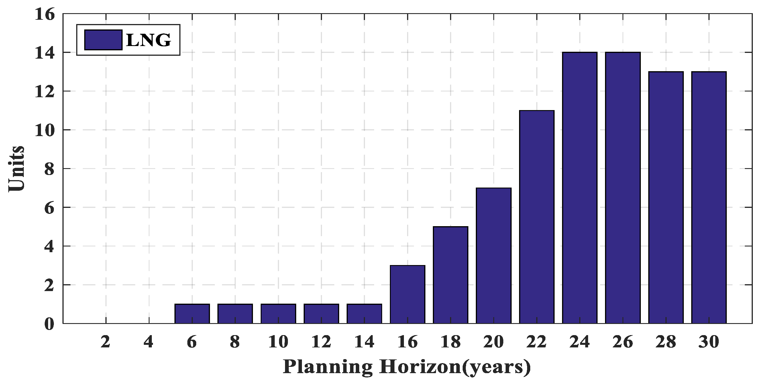
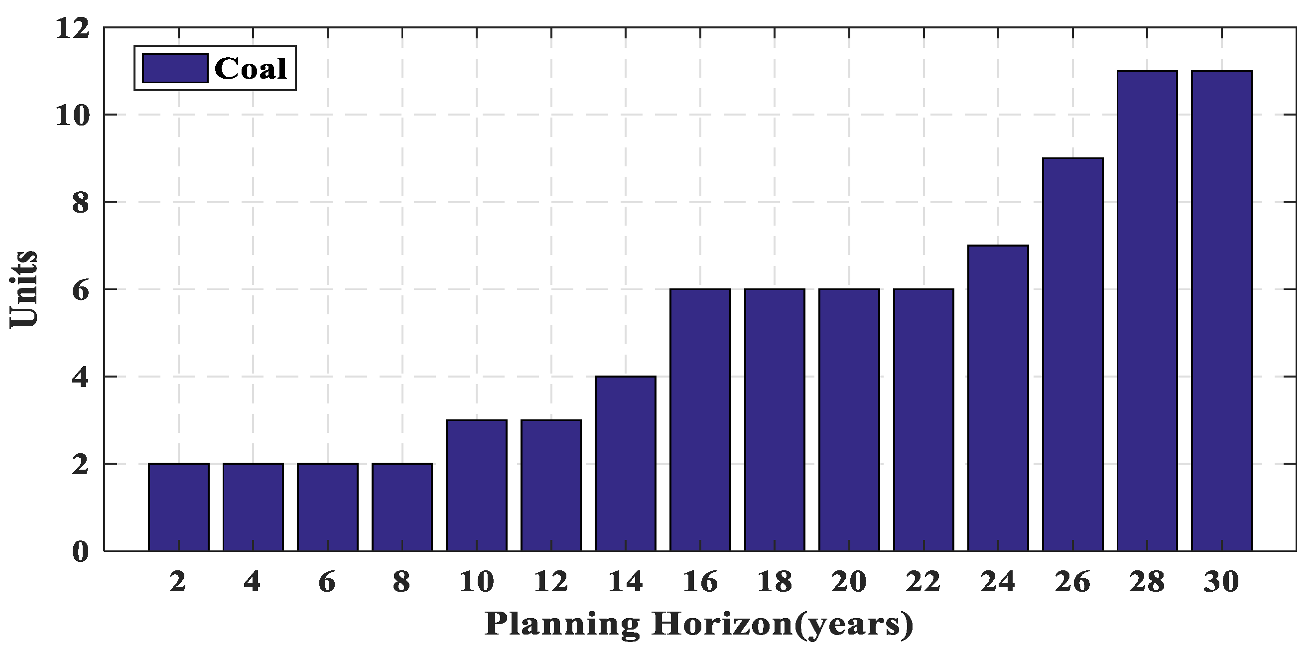
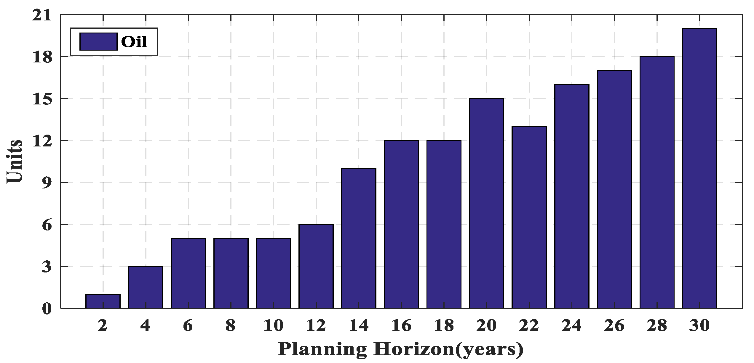
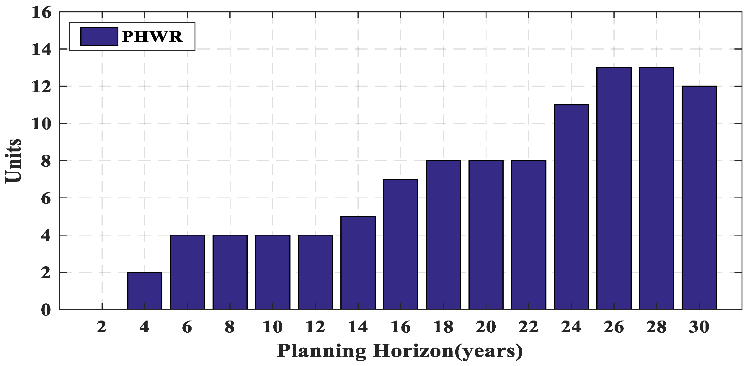
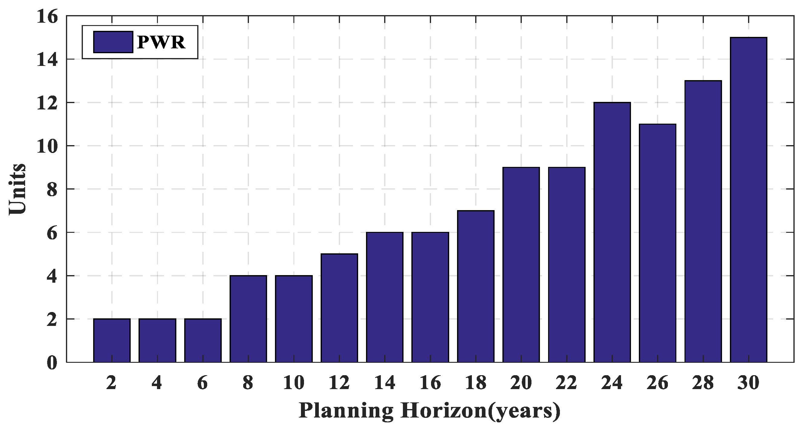
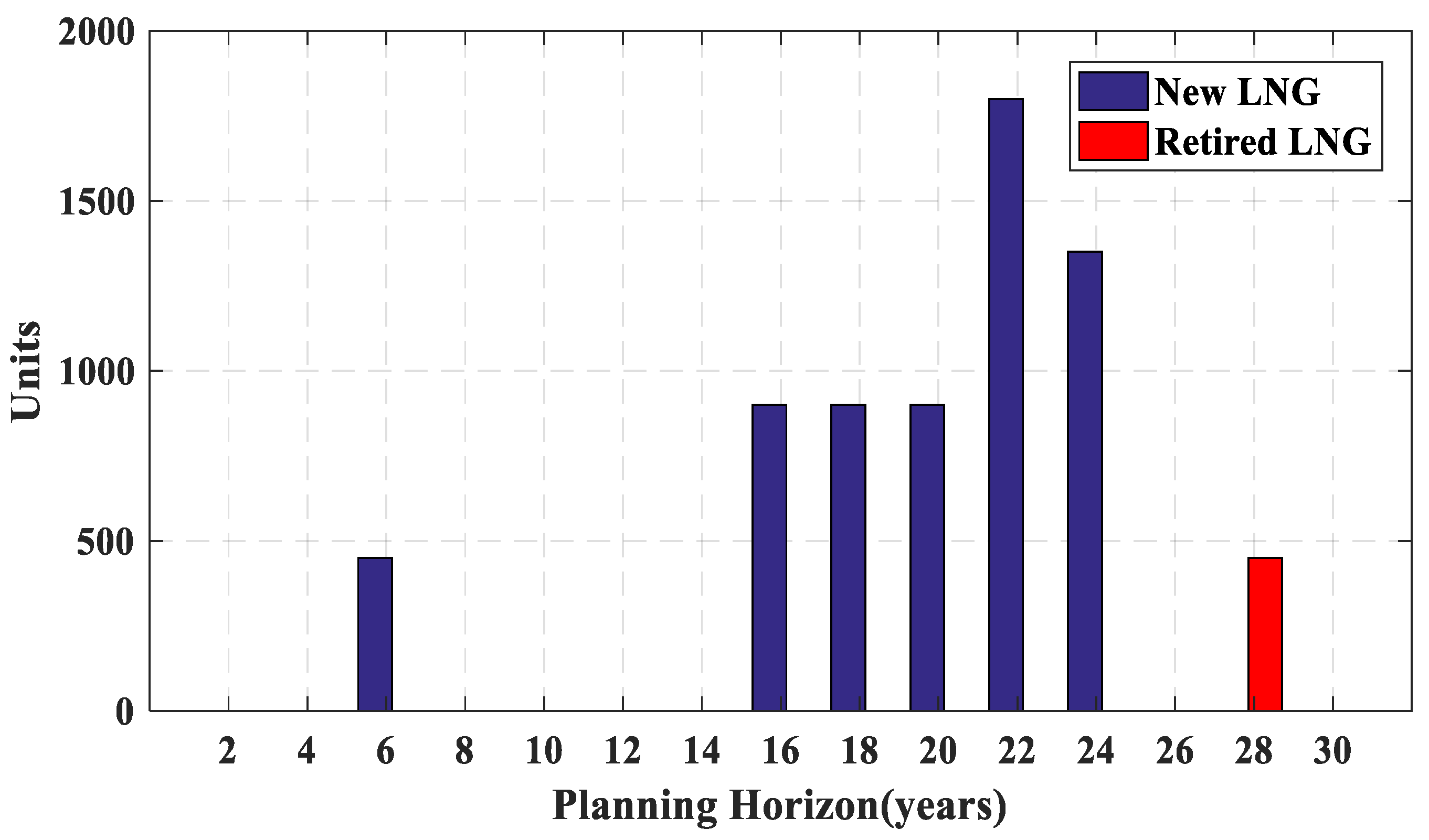
In this paper, the benefits of considering the lifetime constraint on the GEP problem for a 30-year planning horizon have been investigated. Furthermore, since the foundation of GEP studies is based on the annual peak load forecast, a new version of recurrent neural networks known as Bi-directional LSTM networks have been used for forecasting the annual peak load. To show the performance of the BLSTM network, it has been applied on Iran grid data for a test year (2020). The numerical results show the good performance of deep BLSTM which can forecast annual peak load with only 1.22% error in comparison with the real data. To indicate the effect of lifetime constraint, a test system and Iran large-scale power system have been considered as the case studies. The simulation results have shown that after considering the lifetime, sometimes it is not efficient to rebuild retired power plants and another type of power plant should be constructed to meet the demand. In the GEP problem, the power plant(s) of the same type is (are) rebuilt without considering the lifetime constraint. This leads to extra limitations in comparison with the solution, which considers the lifetime constraint. Therefore, the optimal result of the GEP problem with lifetime constraint has less cost. The results of simulations showed that the power plants such as PWR and PHWR, which have low operation costs and high construction, have been constructed in the early years of planning horizon. In contrast, only one LNG power plant has been constructed in the early years of planning horizon due to low construction and high operation cost. In comparison with the total cost of the case, which did not consider the lifetime constraint, the total cost has been decreased by 5.28% and 7.9% after considering the lifetime for the test system and Iran power system, respectively. Moreover, by considering the carbon emission constraint, the total amount of carbon has been decreased by 17%.

Author Contributions

Software, conceptualization, formal analysis, methodology, writing—original draft preparation, investigation, data curation, M.D., M.T., S.S.G.; validation, resources, writing—review and editing, supervision, project administration, funding acquisition, A.N., G.B.G., M.K. All authors have read and agreed to the published version of the manuscript.

Funding

A part of this work has been funded by the Iran National Science Foundation (INSF) project No. 96005975. The funding by INSF is greatly acknowledged by G. B. Gharehpetian.

Institutional Review Board Statement

Not applicable.

Informed Consent Statement

Not applicable.

Conflicts of Interest

The authors declare no conflict of interest.

Nomenclature

Parameters
c1Cognitive component
c2Social component
J Fuel type number
M _ t j Lower bound of j-th fuel type in a year t
M ¯ t j Upper bound of j-th fuel type in a year t
R _ Lower bound of reserve margin
R ¯   Upper bound of reserve margin
T Time period numbers (years) in the planning horizon
U ¯ t Maximum manufactural capacity vector (MW) of generation unit types in a year t
wInertia weight
Ω j Type indicator set of the j-th generation unit
n Total number of input data
n h Total number of hidden units
n o Total number of outputs
r Dimension of each input data sequence
Variables
L t Retired capacity vector (MW) of generation unit types in a year t
L O L P ( X t ) loss of load probability with X t , in a year t
U t Added capacity vector (MW) of generation unit types in a year t
v a ( k ) Velocity of the a-th particle at iteration k
x t i Added capacity (MW) of the i-th unit in a year t
X t Cumulative capacity vector (MW) of generation unit types in a year t
y a ( k ) Position of the a-th particle at iteration k
f t 3 ( L t ) Discounted salvage value ($) due to retired capacity L t in a year t
f t 1 ( U t ) Discounted construction cost ($) due to added capacity U t in a year t
f t 2 ( X t ) Discounted operation and maintenance cost due to cumulative capacity X t in a year t
f t 3 ( X t ) Discounted carbon emission cost due to cumulative capacity X t in a year t
R ( X t ) Capacity reserve margin of X t in a year t
b c , b f , b i , b o Bias vector for cell block, forget gate, input gate, and output gate, respectively
b h ( b ) , b h ( f ) Bias vector for backward and forward hidden layer, respectively
c t , f t , i t Data vector of cell block, forget gate, and input gate at a time t, respectively
c h t , f h t , i h t Data vector of cell block, forget gate, and input gate at a time t in hidden layer, respectively
H t Total hidden vector layers
H t , H t Hidden vector for forward and backward layer at a time t, respectively
o t Data vector of output gate at a time t
O f n Output vector of final layer
o h t Data vector of output gate at a time t in hidden layer
S t State vector of current layer at a state t
S t l State vector of a layer l at a state t
S h t l State vector of a hidden layer l at a state t
W h i , W h φ , W h γ , W h o Weight vector for output of previous state input gate, forget gate, cell block, and output gate, respectively
W i , W i φ , W i γ , W i o Weight vector for input of current state input gate, forget gate, cell block, and output gate, respectively
W h h ( b ) , W h h ( f ) Weight vector of backward and forward layer output data, respectively
W o Weight vector of output layer
W x h ( b ) , W x h ( f ) Weight vector of backward and forward layer input data, respectively
  X t Input data vector at a time t
Indices
aIndex for particle number
i Index for power plant type
j Index for fuel type
k Index for iteration number
t Index for time period
l Index for hidden layer
t Index for time

References

  1. Hemmati, R.; Saboori, H.; Jirdehi, M.A. Multistage generation expansion planning incorporating large scale energy storage systems and environmental pollution. Renew. Energy 2016, 97, 636–645. [Google Scholar] [CrossRef]
  2. Rajesh, K.; Bhuvanesh, A.; Kannan, S.; Thangaraj, C. Least cost generation expansion planning with solar power plant using differential evolution algorithm. Renew. Energy 2016, 85, 677–686. [Google Scholar] [CrossRef]
  3. Valinejad, J.; Marzband, M.; Akorede, M.F.; Barforoshi, T.; Jovanović, M. Generation expansion planning in electricity market considering uncertainty in load demand and presence of strategic GENCOs. Electr. Power Syst. Res. 2017, 152, 92–104. [Google Scholar] [CrossRef] [Green Version]
  4. Jadidoleslam, M.; Ebrahimi, A. Reliability constrained generation expansion planning by a modified shuffled frog leaping algorithm. Int. J. Electr. Power Energy Syst. 2015, 64, 743–751. [Google Scholar] [CrossRef]
  5. Karimyan, P.; Gharehpetian, G.; Abedi, M.; Gavili, A. Long term scheduling for optimal allocation and sizing of DG unit considering load variations and DG type. Int. J. Electr. Power Energy Syst. 2014, 54, 277–287. [Google Scholar] [CrossRef]
  6. Luz, T.; Moura, P.; de Almeida, A. Multi-objective power generation expansion planning with high penetration of renewables. Renew. Sustain. Energy Rev. 2017, 81, 2637–2643. [Google Scholar] [CrossRef]
  7. Flores-Quiroz, A.; Palma-Behnke, R.; Zakeri, G.; Moreno, R. A column generation approach for solving generation expansion planning problems with high renewable energy penetration. Electr. Power Syst. Res. 2016, 136, 232–241. [Google Scholar] [CrossRef]
  8. Maluenda, B.; Negrete-Pincetic, M.; Olivares, D.E.; Lorca, Á. Expansion planning under uncertainty for hydrothermal systems with variable resources. Int. J. Electr. Power Energy Syst. 2018, 103, 644–651. [Google Scholar] [CrossRef]
  9. Kong, X.; Yao, J.; Wang, X. Generation Expansion Planning Based on Dynamic Bayesian Network Considering the Uncertainty of Renewable Energy Resources. Energies 2019, 12, 2492. [Google Scholar] [CrossRef] [Green Version]
  10. Micheli, G.; Vespucci, M.T.; Stabile, M.; Puglisi, C.; Ramos, A. A two-stage stochastic MILP model for generation and transmission expansion planning with high shares of renewables. Energy Syst. 2020, 1–43. [Google Scholar] [CrossRef]
  11. Wang, P.; Wang, C.; Hu, Y.; Varga, L.; Wang, W. Power generation expansion optimization model considering multi-scenario electricity demand constraints: A case study of Zhejiang province, China. Energies 2018, 11, 1498. [Google Scholar] [CrossRef] [Green Version]
  12. Park, H. Generation capacity expansion planning considering hourly dynamics of renewable resources. Energies 2020, 13, 5626. [Google Scholar] [CrossRef]
  13. Haghighi, R.; Yektamoghadam, H.; Dehghani, M.; Nikoofard, A. Generation Expansion Planning Using Game Theory Approach to Reduce Carbon Emission: A Case Study of Iran. Comput. Ind. Eng. 2021, 162, 107713. [Google Scholar] [CrossRef]
  14. Babatunde, O.M.; Munda, J.L.; Hamam, Y. A comprehensive state-of-the-art survey on power generation expansion planning with intermittent renewable energy source and energy storage. Int. J. Energy Res. 2019, 43, 6078–6107. [Google Scholar] [CrossRef]
  15. Oree, V.; Hassen, S.Z.S.; Fleming, P.J. Generation expansion planning optimisation with renewable energy integration: A review. Renew. Sustain. Energy Rev. 2017, 69, 790–803. [Google Scholar] [CrossRef]
  16. Diewvilai, R.; Audomvongseree, K. Generation Expansion Planning with Energy Storage Systems Considering Renewable Energy Generation Profiles and Full-Year Hourly Power Balance Constraints. Energies 2021, 14, 5733. [Google Scholar] [CrossRef]
  17. Dagoumas, A.S.; Koltsaklis, N.E. Review of models for integrating renewable energy in the generation expansion planning. Appl. Energy 2019, 242, 1573–1587. [Google Scholar] [CrossRef]
  18. Rajesh, K.; Kannan, S.; Thangaraj, C. Least cost generation expansion planning with wind power plant incorporating emission using differential evolution algorithm. Int. J. Electr. Power Energy Syst. 2016, 80, 275–286. [Google Scholar] [CrossRef]
  19. Jin, S.; Ryan, S.M.; Watson, J.-P.; Woodruff, D.L. Modeling and solving a large-scale generation expansion planning problem under uncertainty. Energy Syst. 2011, 2, 209–242. [Google Scholar] [CrossRef]
  20. Gitizadeh, M.; Kaji, M.; Aghaei, J. Risk based multiobjective generation expansion planning considering renewable energy sources. Energy 2013, 50, 74–82. [Google Scholar] [CrossRef]
  21. Sun, D.; Xie, X.; Wang, J.; Li, Q.; Wei, C. Integrated generation-transmission expansion planning for offshore oilfield power systems based on genetic Tabu hybrid algorithm. J. Mod. Power Syst. Clean Energy 2017, 5, 117–125. [Google Scholar] [CrossRef] [Green Version]
  22. Park, J.-B.; Park, Y.-M.; Won, J.-R.; Lee, K.Y. An improved genetic algorithm for generation expansion planning. IEEE Trans. Power Syst. 2000, 15, 916–922. [Google Scholar] [CrossRef] [Green Version]
  23. Foley, A.; Gallachóir, B.Ó. Analysis of electric vehicle charging using the traditional generation expansion planning analysis tool WASP-IV. J. Mod. Power Syst. Clean Energy 2015, 3, 240–248. [Google Scholar] [CrossRef] [Green Version]
  24. Koltsaklis, N.E.; Georgiadis, M.C. A multi-period, multi-regional generation expansion planning model incorporating unit commitment constraints. Appl. Energy 2015, 158, 310–331. [Google Scholar] [CrossRef]
  25. Palmintier, B.; Webster, M. Impact of unit commitment constraints on generation expansion planning with renewables. In Proceedings of the 2011 IEEE Power and Energy Society General Meeting, Detroit, MI, USA, 24–28 July 2011; pp. 1–7. [Google Scholar]
  26. Palmintier, B.S.; Webster, M.D. Impact of operational flexibility on electricity generation planning with renewable and carbon targets. IEEE Trans. Sustain. Energy 2015, 7, 672–684. [Google Scholar] [CrossRef]
  27. Tohidi, Y.; Aminifar, F.; Fotuhi-Firuzabad, M. Generation expansion and retirement planning based on the stochastic programming. Electr. Power Syst. Res. 2013, 104, 138–145. [Google Scholar] [CrossRef]
  28. Mavalizadeh, H.; Ahmadi, A.; Gandoman, F.H.; Siano, P.; Shayanfar, H.A. Multiobjective robust power system expansion planning considering generation units retirement. IEEE Syst. J. 2017, 12, 2664–2675. [Google Scholar] [CrossRef]
  29. Mejía Giraldo, D.A.; López Lezama, J.M.; Gallego Pareja, L.A. Power system capacity expansion planning model considering carbon emissions constraints. Rev. Fac. Ing. Univ. Antioq. 2012, 62, 114–125. [Google Scholar]
  30. Doagou-Mojarrad, H.; Rastegar, H.; Gharehpetian, G.B. Probabilistic interactive fuzzy satisfying generation and transmission expansion planning using fuzzy adaptive chaotic binary PSO algorithm. J. Intell. Fuzzy Syst. 2016, 30, 1629–1641. [Google Scholar] [CrossRef]
  31. Yao, W.; Chung, C.; Wen, F.; Qin, M.; Xue, Y. Scenario-based comprehensive expansion planning for distribution systems considering integration of plug-in electric vehicles. IEEE Trans. Power Syst. 2015, 31, 317–328. [Google Scholar] [CrossRef]
  32. Suriya, P.; Subramanian, S.; Ganesan, S.; Hariprasath, M. Multi-objective generation expansion and retirement planning using chaotic grasshopper optimisation algorithm. Aust. J. Electr. Electron. Eng. 2019, 16, 136–148. [Google Scholar] [CrossRef]
  33. Jahangir, H.; Gougheri, S.S.; Vatandoust, B.; Golkar, M.A.; Ahmadian, A.; Hajizadeh, A. Plug-in Electric Vehicle Behavior Modeling in Energy Market: A Novel Deep Learning-Based Approach with Clustering Technique. IEEE Trans. Smart Grid 2020, 11, 4738–4748. [Google Scholar] [CrossRef]
  34. Mishra, M.; Nayak, J.; Naik, B.; Abraham, A. Deep learning in electrical utility industry: A comprehensive review of a decade of research. Eng. Appl. Artif. Intell. 2020, 96, 104000. [Google Scholar] [CrossRef]
  35. Jahangir, H.; Tayarani, H.; Gougheri, S.S.; Golkar, M.A.; Ahmadian, A.; Elkamel, A. Deep Learning-based Forecasting Approach in Smart Grids with Micro-Clustering and Bi-directional LSTM Network. IEEE Trans. Ind. Electron. 2020, 68, 8298–8309. [Google Scholar] [CrossRef]
  36. Rhode, S.; Van Vaerenbergh, S.; Pfriem, M. Power prediction for electric vehicles using online machine learning. Eng. Appl. Artif. Intell. 2020, 87, 103278. [Google Scholar] [CrossRef]
  37. Chen, Q.; Kang, C.; Xia, Q.; Zhong, J. Power generation expansion planning model towards low-carbon economy and its application in China. IEEE Trans. Power Syst. 2010, 25, 1117–1125. [Google Scholar] [CrossRef] [Green Version]
  38. Valinejad, J.; Marzband, M.; Elsdon, M.; Saad Al-Sumaiti, A.; Barforoushi, T. Dynamic carbon-constrained EPEC model for strategic generation investment incentives with the aim of reducing CO2 emissions. Energies 2019, 12, 4813. [Google Scholar] [CrossRef] [Green Version]
  39. Sun, J.; Liu, L.; Liu, Y.; Shi, F. Low-Carbon Generation Expansion Planning Based on the Global Energy Interconnection Construction Plan. In Proceedings of the 2020 IEEE/IAS Industrial and Commercial Power System Asia (I&CPS Asia), Weihai, China, 13–15 July 2020; pp. 805–809. [Google Scholar]
  40. Hu, Y.; Ding, T.; Bie, Z.; Lian, H. Integrated generation and transmission expansion planning with carbon capture operating constraints. In Proceedings of the 2016 IEEE Power and Energy Society General Meeting (PESGM), Boston, MA, USA, 17–21 July 2016; pp. 1–5. [Google Scholar]
  41. Pourmoosavi, M.-A.; Amraee, T. Low carbon generation expansion planning with carbon capture technology and coal phase-out under renewable integration. Int. J. Electr. Power Energy Syst. 2021, 128, 106715. [Google Scholar] [CrossRef]
  42. Asgharian, V.; Abdelaziz, M. A low-carbon market-based multi-area power system expansion planning model. Electr. Power Syst. Res. 2020, 187, 106500. [Google Scholar] [CrossRef]
  43. Jahangir, H.; Tayarani, H.; Ahmadian, A.; Golkar, M.A.; Miret, J.; Tayarani, M.; Gao, H.O. Charging demand of plug-in electric vehicles: Forecasting travel behavior based on a novel rough artificial neural network approach. J. Clean. Prod. 2019, 229, 1029–1044. [Google Scholar] [CrossRef]
  44. Makarenkov, V.; Rokach, L.; Shapira, B. Choosing the right word: Using bidirectional LSTM tagger for writing support systems. Eng. Appl. Artif. Intell. 2019, 84, 1–10. [Google Scholar] [CrossRef] [Green Version]
  45. Huang, C.-G.; Huang, H.-Z.; Li, Y.-F. A bidirectional LSTM prognostics method under multiple operational conditions. IEEE Trans. Ind. Electron. 2019, 66, 8792–8802. [Google Scholar] [CrossRef]
  46. Lin, J.C.-W.; Shao, Y.; Zhou, Y.; Pirouz, M.; Chen, H.-C. A Bi-LSTM mention hypergraph model with encoding schema for mention extraction. Eng. Appl. Artif. Intell. 2019, 85, 175–181. [Google Scholar] [CrossRef]
  47. Liu, J.; Wang, Z.; Xu, M. DeepMTT: A deep learning maneuvering target-tracking algorithm based on bidirectional LSTM network. Inf. Fusion 2020, 53, 289–304. [Google Scholar] [CrossRef]
  48. Neshat, N.; Amin-Naseri, M. Cleaner power generation through market-driven generation expansion planning: An agent-based hybrid framework of game theory and particle swarm optimization. J. Clean. Prod. 2015, 105, 206–217. [Google Scholar] [CrossRef]
Figure 1. Construction of LSTM block.
Energies 14 08035 g001
Figure 2. BLSTM network structure.
Energies 14 08035 g002
Figure 3. Number of LNG-fired power plants during planning horizon.
Energies 14 08035 g003
Figure 4. Number of coal-fired power plants during planning horizon.
Energies 14 08035 g004
Figure 5. Number of oil-fired power plants during planning horizon.
Energies 14 08035 g005
Figure 6. Number of nuclear power plants during planning horizon.
Energies 14 08035 g006
Figure 7. Number of nuclear power plants (PWR) during planning horizon.
Energies 14 08035 g007
Figure 8. Capacity installed (blue bars) or retired (red bars) in each year for LNG-fired power plants.
Energies 14 08035 g008
Figure 9. Capacity installed (blue bars) or retired (red bars) in each year for coal-fired power plants.
Energies 14 08035 g009
Figure 10. Capacity installed (blue bars) or retired (red bars) in each year for nuclear power plants (PHWR).
Energies 14 08035 g010
Figure 11. Capacity installed (blue bars) or retired (red bars) in each year for oil-fired power plants.
Energies 14 08035 g011
Figure 12. Capacity installed (blue bars) or retired (red bars) in each year for nuclear power plants (PWR).
Energies 14 08035 g012
Figure 13. Daily forecasted peak load for July to September 2020 by different methods and their yearly peak loads.
Energies 14 08035 g013
Figure 14. Number of biomass power plants of Iran power system during planning horizon.
Energies 14 08035 g014
Figure 15. Number of natural gas-fired power plants of Iran power system during planning horizon.
Energies 14 08035 g015
Figure 16. Number of photovoltaic power plants of Iran power system during planning horizon.
Energies 14 08035 g016
Figure 17. Number of solar power plants of Iran power system during planning horizon.
Energies 14 08035 g017
Figure 18. Number of wind power plants of Iran power system during planning horizon.
Energies 14 08035 g018
Figure 19. Number of combined cycle power plants of Iran power system during planning horizon.
Energies 14 08035 g019
Figure 20. The total cumulative capacity of each power plant in the last year.
Energies 14 08035 g020
Table 2. Technical and economic data of existing plants of test system.
NameNo. of UnitsUnit Capacity (MW)Operating Cost ($/kWh)Fixed O&M Cost
($/kW-mon)
Oil 112000.0242.25
Oil 212000.0272.25
Oil 311500.0302.13
LNG G/T3500.0434.52
LNG C/C 114000.0381.63
LNG C/C 214000.0401.63
LNG C/C 314500.0352.00
Coal 122500.0236.65
Coal 215000.0192.81
Coal 315000.0152.81
PWR 1110000.0054.94
PWR 2110000.0054.63
Table 3. Forecasted peak demand of test system.
YearPeak (MW)YearPeak (MW)
050001617,000
270001818,000
490002020,000
610,0002222,000
812,0002424,000
1013,0002626,000
1214,0002827,000
1415,0003030,000
Table 4. Technical and economic data of candidate plants of test system.
Candidate TypeOilLNGCoalPWRPHWR
Construction upper limit54333
Capacity (MW)2004505001000700
Operating cost ($/kWh)0.0210.0350.0140.0040.003
Fixed O&M cost ($/kW-mon)2.200.902.754.605.50
Capital cost ($/kW)812.5500.01062.51625.01750.0
Lifetime (years)2022242628
Table 5. Remaining lifetime of existing power plants of test system.
Name
(Fuel Type)
Lifetime (years)Name
(Fuel Type)
Lifetime (years)
Oil 16LNG C/C 320
Oil 210Coal 18
Oil 314Coal 212
LNG G/T4Coal 316
LNG C/C 110PWR 112
LNG C/C 216PWR 216
Table 6. Number of retired and new power plants of test system.
YearOilLNGPWRCoal
NewRetiredTotalNewRetiredTotalNewRetiredTotalNewRetiredTotal
2101000202202
4203000002002
6205101002002
8005001204002
10005001004103
12106001105003
144010001106104
162012203006206
180012205107006
204115207209006
2202134011009006
24521630143012327
26101700141211209
281018011320132011
303120001320150011
Table 7. Total cost of test system with and without considering lifetime.
MethodTotal Cost (M $)
Without considering lifetime40,248
With considering lifetime38,231
Table 8. Error criteria of forecasted results for daily peak load from July to September 2020.
Error Criterion
MAPE (%)MAE (MW)RMSE (MW)
BLSTM1.901031.741276.69
LSTM2.291243.791515.57
MLP3.571942.652437.11
Table 9. Forecasted peak demand of Iran power system by BLSTM.
YearPeak (MW)YearPeak (MW)
160,4791680,180
262,6131780,685
364,6441882,143
466,5601982,812
568,3542083,446
670,0212185,632
771,5582286,143
872,9672389,231
974,2482491,968
1075,4082592,457
1176,4512692,967
1277,3842792,692
1378,2162893,619
1478,9542994,276
1579,6063095,889
Table 10. Technical and economic data of candidate and existing plants of Iran power system.
TypeInvestment (1000 Rial/kW)O&M Cost (Rial/kWh)CO2 Generation Rate (ton CO2/MWh)Existing Capacity (MW)Plant Life (year)Unit Size (MW)
Nuclear87,990315000601000
Coal based80,70029250.4040320
Combined cycle20,4112930.3414,63220480
Natural gas12,7503900.521,61715162
Steam based24,4504500.7115,70430320
Hydroelectric48,9204940954250100
Wind56,430103.20902225
Solar92,700171.90020100
Photovoltaic135,00027.30015100
Biomass121,5001350002025
Table 11. Total cost of Iran power system with and without considering lifetime.
MethodTotal Cost (M Rial)
Without considering lifetime9.54 × 109
With considering lifetime8.84 × 109
Table 12. Retired and new power plants of Iran power system.
Biomass Natural Wind Photovoltaic
YearNewRetiredTotalNewRetiredTotalNewRetiredTotalNewRetiredTotal
160039062610490634
172041132400490034
180041002400490430
190041262000493033
201042532250543630
211637302530575629
223040552510580524
235441142256574424
246641602866576030
253638303136541229
263635213213521129
276338613760586233
280137113726540033
295042013655543036
303243413934533435
Table 13. Total carbon produced by Iran power system with and without considering carbon emissions constraint.
MethodTotal Carbon (Ton)
Without considering the carbon emission constraint1.5492 × 106
With considering the carbon emission constraint1.2731 × 106
Publisher’s Note: MDPI stays neutral with regard to jurisdictional claims in published maps and institutional affiliations.

