
Cascade Control of the Ground Station Module of an Airborne Wind Energy System
by
 , , and
Ali Arshad Uppal
1,2 ,
,
Manuel C. R. M. Fernandes
1 ,
,
Sérgio Vinha
1 and
Fernando A. C. C. Fontes
1,* 1
SYSTEC and Department of Electrical and Computer Engineering, Faculty of Engineering, Universidade do Porto, 4099-002 Porto, Portugal
2
Department of Electrical and Computer Engineering, COMSATS University Islamabad, Islamabad 45550, Pakistan
*
Author to whom correspondence should be addressed.
Energies 2021, 14(24), 8337; https://0-doi-org.brum.beds.ac.uk/10.3390/en14248337
Submission received: 1 November 2021
/
Revised: 30 November 2021
/
Accepted: 2 December 2021
/
Published: 10 December 2021
(This article belongs to the Special Issue Airborne Wind Energy Systems)
Abstract
:An airborne wind energy system (AWES) can harvest stronger wind streams at higher altitudes which are not accessible to conventional wind turbines. The operation of AWES requires a controller for the tethered aircraft/kite module (KM), as well as a controller for the ground station module (GSM). The literature regarding the control of AWES mostly focuses on the trajectory tracking of the KM. However, an advanced control of the GSM is also key to the successful operation of an AWES. In this paper we propose a cascaded control strategy for the GSM of an AWES during the traction or power generation phase. The GSM comprises a winch and a three-phase induction machine (IM), which acts as a generator. In the outer control-loop, an integral sliding mode control (SMC) algorithm is designed to keep the winch velocity at the prescribed level. A detailed stability analysis is also presented for the existence of the SMC for the perturbed winch system. The rotor flux-based field oriented control (RFOC) of the IM constitutes the inner control-loop. Due to the sophisticated RFOC, the decoupled and instantaneous control of torque and rotor flux is made possible using decentralized proportional integral (PI) controllers. The unknown states required to design RFOC are estimated using a discrete time Kalman filter (DKF), which is based on the quasi-linear model of the IM. The designed GSM controller is integrated with an already developed KM, and the AWES is simulated using MATLAB and Simulink. The simulation study shows that the GSM control system exhibits appropriate performance even in the presence of the wind gusts, which account for the external disturbance.

1. Introduction
The kinetic energy of wind tends to increase with altitude and is much higher at altitudes between 0.5–12 km above the ground than in the proximity of the surface, cf. [1]. In order to exploit these abundant wind resources, the wind turbine manufacturers are constantly working to increase the size of wind turbine systems. However, such scaling-up of the systems requires more material for tower structure and foundations, which results in an increased cost. Apart from financial constraints there are also some physical constraints that limit the size of a wind turbine. There is a consensus that such higher-altitude winds, even 500 m, cannot be reached by any towered turbine without a radical change of concept. In this scenario, airborne wind energy systems (AWES) aim at playing a vital role to convert wind at higher altitudes to electricity. The seminal work of Loyd, cf. [2] paved the way for the development of AWESs. He computed the maximum energy extracted from AWESs with tethered wings. The main concept of AWES can be illustrated by the idea of replacing the tips of blades of a wind turbine by a tethered airfoil, e.g., a soft kite or rigid wing, which is connected to a ground station, cf. [3,4].
AWES can be classified into two major classes: Ground-gen AWES (GG-AWES) and fly-gen AWES (FG-AWES), depending on where the electricity is generated, cf. [4,5]. In GG-AWES, the tether provides the mechanical energy to the generator housed in the ground station. Whereas, in Fly-Gen systems the electricity is generated on board the flying device. In this type of AWES, the tether is used to conduct electricity from the aircraft to the ground station. GG-AWES are further classified as fixed and moveable GG-AWES, and both types are extensively used by industrial and academic researchers. In this research we focus on fixed GG-AWES that are operated in pumping cycle. A pumping kite generator operates in two phases: Traction (generation phase) and retraction (recovery phase). In traction mode the electricity is generated and in retraction phase, a small amount of energy is consumed. The tether which is connected to the drone/kite/aircraft and the ground station is wound on a winch, which is connected to the rotor of an electric machine. In traction mode, the aircraft is driven in a crosswind flight. The lift produced by the aircraft induces tractive force on the tether and consequently mechanical energy is provided to the electrical machine, which acts as a generator. In retraction phase, the machine acts as a motor and rewinds the tether, bringing the aircraft down. The energy produced in the traction phase should be significantly greater than the energy consumed in the retraction mode. The most efficient paths during the crosswind flight are circular or figure-of-eight for maximum power production, cf. [4,6,7]. This is guaranteed by designing a sophisticated control system for an AWES.
1.1. Related Work
Two main objectives of an AWES control system are maximizing the power generation and maintaining a safe and reliable operation, cf. [7,8]. These sometimes conflicting goals are achieved by the automatic control of AWES. However, the time varying and uncertain nature of the wind at the time scale of interest make the feedback control of AWES a formidable task. In normal operating conditions, an AWES control system needs to manage three distinct operational phases: Launch, power generation, and landing. Moreover, the control system needs to ensure smooth inter phase transitions, cf. [7]. The operational phases of an AWES differ significantly in terms of operating conditions and control objectives, therefore, every phase has its own local control strategy to achieve a certain control objective. In order to ensure co-operation between the ground station and on-board kite controllers, a supervisory control is employed which manages the switching between different operational phases. Owing to the contradicting control objectives for different operational phases of an AWES, the overall control of AWES is quite challenging and there is considerable room to improve upon existing literature. In [6], the authors have conducted a pioneering work for the control of AWES in all operational modes, which includes take-off, transition to power generation, pumping energy generation cycles, transition to hovering, and landing.
Most of the literature pertaining to the AWES control deals with the control of crosswind flight and pumping operation. In pumping action control, the preferred reference trajectory for traction phase is a figure-of-eight or circular/elliptical path, whereas, in retraction phase the reference path is a straight line. A common strategy for the control of the kite in crosswind flight is discussed in [9,10,11,12]. In this technique, a continuous Lemniscate parametrization is chosen for the figure-of-eight path. The path can be discretized to obtain a fixed number of waypoints along the path, cf. [13,14]. Other techniques are more abstract, which calculate the desired flight direction either by determining the current active waypoint or reference point on the path, cf. [15]. Apart from the pumping cycle control, a fully autonomous AWES also requires an efficient control of launch and landing phases. An AWES can be launched whenever the environmental conditions are favorable to generate electricity. However, the landing phase is more technical: The aircraft needs to be landed when the conditions are not suitable for electricity generation or there is a fault in the system. The system level launch and land strategies have been explored in [16,17], whereas, specific solutions and phases are discussed in [6,18,19]. In most of the above techniques, it has been assumed that the states required for the synthesis of model-based control are directly available for measurement. However, this assumption is not realistic. In the literature, several approaches have been proposed for an unknown state and parameter estimation pertaining to AWES, and for reducing the effect of sensor noise, cf. [20,21].
One of the major objectives of an AWES control is to maximize the output power. This can be achieved by realizing performance levels as close to the theoretical limits of Loyd’s work in [2] as possible. This needs to be achieved while respecting several operational constraints. In this scenario the role of optimization and hence optimal control is very pertinent to AWES. Therefore, several approaches have been reported in the literature, which include offline optimal control for performance prediction, cf. [22,23,24,25]; model predictive control (MPC): For pumping mode AWES, cf. [26], for real-time simulation studies, cf. [27], and robust MPC, cf. [28]; and adaptive control techniques: Extremum seeking control, cf. [29] and iterative learning control, cf. [30].
As compared to the control of KM, the control of electric machine pertaining to GSM is not discussed by many researchers. The contributions of Hisham et al. [31,32] provide a detailed account on the fault tolerant control of electrical drives for GG-AWES. In order to keep a higher efficiency of the electric machine during the pumping cycle, the concept of dual three phase machines (DTMs) is used. The idea is demonstrated using interior permanent magnet synchronous machine (IPMSM), which is rewinded as a DTM. In [33], the authors design power control strategies for controlling the active and reactive power of an AWE farm.
1.2. Research Gap
Two fundamental components of GG-AWES are the ground station module (GSM) and the kite module (KM). The GSM comprises a winch, an electrical machine, and their respective control systems, whereas, the aircraft/drone and its on-board controllers constitute the KM. As discussed above, the literature regarding the control of AWES mainly focuses on the trajectory control of aircraft in a pumping cycle. An advanced control of the GSM and its integration with the KM controllers have not been fully discussed in the literature. In [6], the authors propose a comprehensive control strategy for all operational phases of AWES. However, the control of the GSM is based on a simplified winch-machine model. An electric machine has a pivotal role in the success of an AWES. In [31], an efficient fault tolerant control of electric drives pertaining to GG-AWES is discussed, however, the focus is not on the coupling of the electric machine with winch and the KM. A cascade control strategy for the electric machine and winch is required to provide a desired winch velocity to the KM.
1.3. Major Contributions
In this manuscript we propose a cascaded control of the GSM during the traction or power-production phase. The GSM, together with the KM, form the two main components of the AWES. The focus of research work is the GSM and the development of its controllers therefore, the KM is considered as a black box which takes the winch velocity as the input and yields tether force as the output. For simulations, we use known models and algorithms for the KM and its controller, namely the the ones in [34,35].
The GSM comprises a winch and a 3-phase induction machine (IM), which can operate either as a motor or as a generator. The cascaded GSM controller provides the desired reel-out winch velocity to KM in traction phase. The GSM control strategy is composed of inner and outer feedback loops. The slower outer-loop represents the winch speed control system, whereas, the faster, inner control-loop is for obtaining the desired torque of the IM. A model-based robust sliding mode control (SMC) algorithm, cf. [36] is used to design the winch speed controller. A detailed stability analysis is also provided for the SMC controller for the perturbed winch system. On the other hand, the control of the IM is based on its 2-phase model, cf. [37,38]. For the high performance control of the IM, the rotor flux oriented control (RFOC), cf. [39] technique is used, which enables a DC machine-like control of the two phase IM model. By virtue of RFOC, the torque and flux control problem is decoupled in such a way that the decentralized control of both torque and flux is possible. Moreover, both torque and flux of the IM can be controlled instantaneously. The decentralized controllers are of the proportional-integral (PI) type. The torque controller tracks the desired trajectory of the torque which is required to obtain a desired winch speed. Whereas, the flux controller tracks an optimum flux trajectory, which minimizes the losses in the IM. It is pertinent to mention here that the unknown states of the IM, which are used in RFOC are estimated using a discrete-time Kalman filter (DKF), which is based on the quasi-linear model of IM, cf. [40]. The conventional linearization based on the Taylor series expansion only gives the approximation of the non-linear system around a fixed operating point, therefore, the linear system is valid in a small operating range. On the other hand, the quasi-linear approach transforms the non-linear system into a state-space form comprising state dependent matrices. Moreover, the exact non-linear dynamics of the system remains intact. Subsequently, the estimation of unknown states is improved. To evaluate the performance of the proposed strategy, the simulations are performed in Matlab/Simulink. The already developed strategy of [34] is used to simulate and analyze the KM. The simulation results show that AWES demonstrates the desired performance, even in the presence of external disturbance in the form of wind gusts.
The remaining article is organized in the following manner. A detailed discussion on the mathematical models of the winch and IM is presented in Section 2. The cascaded control of the GSM is discussed in Section 3. The results are discussed and presented in Section 4 and the article is concluded in Section 5.
2. Modeling of Ground Station Module
As discussed earlier, the GSM is composed of a winch and an IM. The objective of this module is to operate KM at the prescribed velocity, which depends upon the operating phase of an AWES. In this section the control-oriented mathematical models of a winch and IM are discussed.
2.1. Mathematical Model of Winch
The application of the Newton’s second law of rotation on the winch yields (cf. [6]):
where , , , and are the inertia, damping coefficient, rotational speed, and radius of winch, respectively; and represent tether force and IM torque, respectively; and is the unknown norm bounded disturbance: , which accounts for the torque generated by the wind gusts.
and are exogenous inputs with reference to the winch. The positive sign with in (1) shows that the winch is providing mechanical power to the IM, which is acting as a generator.
2.2. Mathematical Model of Induction Machine
The dynamic behavior of an IM is complex because the rotor is rotating with respect to the stationary stator. Due to the rotation of the rotor, the coupling coefficients become a function of the rotor position, therefore, the mathematical model of the IM becomes time varying, rendering it difficult for control and estimation applications. For obtaining a control-oriented model of an IM, a reference frame transformation is carried out, which essentially converts a three-phase () machine into its two-phase () equivalent model, where d refers to the direct and q represents the quardature axis. It is pertinent to mention here that the d and q axes are orthogonal to each other. The IM models are categorized as stationary and synchronously rotating reference frame models. In the stationary reference frame (SRF), the coordinate system does not rotate and is fixed in the stator of the machine. Whereas in a synchronously rotating reference frame (SRRF), the coordinate system rotates with synchronous speed (), cf. [38]. Throughout this article, the quantities in SRF are represented by superscript s, while the SRRF variables do not have any superscript.
The conversions between and IM models are possible by employing Clarke’s and Park’s transformations, cf. [39]. The first step in RFOC is to convert the IM model into a SRF model by applying Clarke’s transformation as:
where , , and represent an arbitrary quantity (current, flux or voltage) in symmetrical (the phases are exactly 120 apart from each other) axes, respectively; and represent axes quantities in SRF, respectively; and is the angle between and . We are assuming that the system is balanced, therefore, the neutral quantity .
Subsequently Park’s transformation is used in the following manner to convert SRF to SRRF:
where is the angle between and .
It is pertinent to mention here that both rotation matrices used in (2) and (3) are invertible, hence inverse transformations are also possible and are required during different stages of RFOC.
Both models of an IM, i.e., SRRF and SRF are employed for designing a model-based RFOC. The controller design is carried out using the SRRF model, whereas, the flux estimator is based on the SRF model. The mathematical models of IM in SRRF and SRF are given below.
2.2.1. Model of an Induction Machine in Synchronously Rotating Reference Frame
The mathematical model of the IM in SRRF is adapted from [41,42], and is given as:
where and represent axes currents of stator windings in SRRF, respectively; and represent the rotor fluxes in SRRF, respectively; and represent axes stator voltages in SRRF, respectively; and is the electrical speed of the rotor. The constants depend on the construction of the machine and are given as:
where and are resistances of rotor and stator windings, respectively; and , , and represent the rotor, stator, and magnetizing inductances, respectively.
The electrical speed of the rotor used in the SRRF model in (4) can be obtained by typical mechanical loading of the motors, and is characterized by:
where J and b are equivalent rotor inertia and damping coefficient, respectively, and and are electromagnetic and load torques, respectively. The expression for in SRRF is given as:
where denotes the number of pole pairs.
The mechanical () and electrical speeds of the rotor are related through the number of pole pairs as:
2.2.2. Model of an Induction Machine in Stationary Reference Frame
In SRF, the synchronous speed . The differential equations for the currents and fluxes for the squirrel cage induction machine are given as:
2.3. Coupling of Winch and Induction Machine
The winch and the IM are coupled using the gear train. In order to avoid the complexity, a linearized interaction is considered between the winch and IM gears (cf. Figure 1). The relationship between the winch and IM torques is given as:
where , , , , and represent reference torque trajectory of IM, torque produced by the winch speed controller, input torque to the winch, number of teeth of IM gear, and number of teeth of winch gear, respectively.
The gears are used to provide a mechanical advantage to IM, so that it can drive a heavier load. To make this possible, a bigger gear is used on the winch side as compared to the IM gear, i.e., .
3. Cascade Control Strategy for Ground Station Module
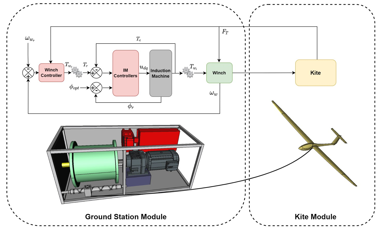
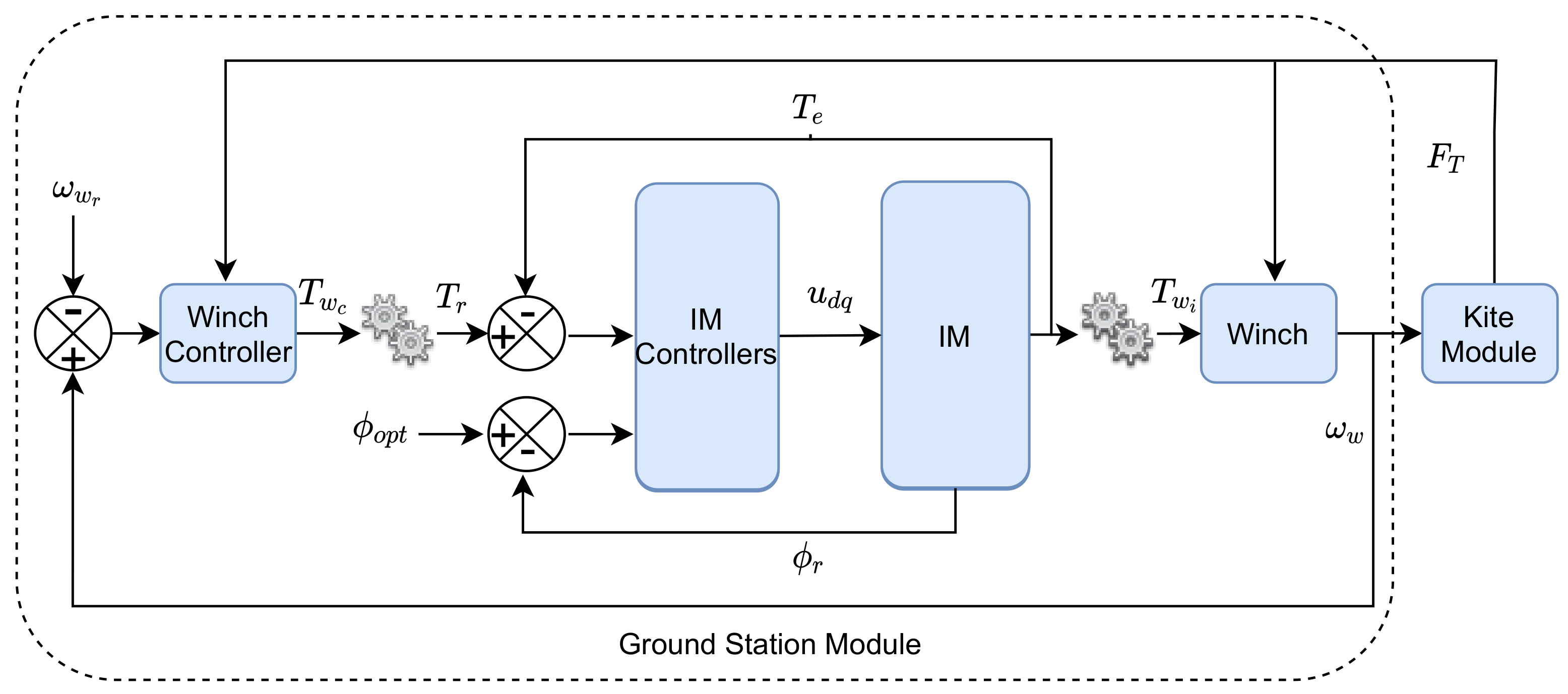
As mentioned earlier, the objective of the GSM is to operate KM at the prescribed velocity, which depends upon the operating phase of an AWES. For this purpose, a winch speed control system is designed to maintain a prescribed speed of the winch during the traction phase. This is only possible by designing a cascade control system as shown in Figure 1. The symbols , , , , , , , , and represent reference winch velocity, output torque of winch speed controller, reference induced torque of the IM, induced torque of the IM, input torque of the winch, tether force, winch velocity, rotor flux, optimal rotor flux and axes stator control voltages, respectively. The interaction between the winch and IM controllers is made in such a way that the torque provide to the IM (IM acting as a generator) has such a time profile that the desired winch speed can be attained. In Figure 1, the inner loop contains the IM torque controller and the winch speed control system is in the outer loop. As a general rule of thumb, the bandwidth of the inner control loop, i.e., IM control system needs to be 10 times faster as compared to the outer loop for the winch speed control. This is required to ensure that the IM provides the required torque almost instantly, needed to attain the desired winch velocity. As discussed earlier, the interaction between GSM and KM is through the winch, as the tether attached to the kite is wound on the winch. The detail of the IM and winch speed controllers is provided in the subsequent text.
3.1. Sliding Mode Control Design for Winch System
A conventional SMC is designed for the winch model given in (1). The first step in SMC design is the selection of a sliding variable. In order to keep at the desired value , a proportional integral (PI) type sliding variable is selected as:
where is a design parameter and is the winch speed tracking error.
To ensure the finite time convergence of the system trajectories to the sliding manifold the following reachability condition is selected, cf. [43]:
where represents the discontinuous controller gain.
After computing the time derivative of (10) and substituting in (11), we can obtain the following expression for the output torque () of the winch speed controller.
In order to show that the control law given in (12) drags the system trajectories to the manifold in finite time, a Lyapunov functional is selected as follows:
Taking the time derivative of the Lyapunov functional in (13) along the trajectories of (1), we get:
where represents the dynamics of the perturbed winch system, including the effect of unknown .
According to [44], the result in (15) ensures that the trajectories of the perturbed winch system in (1) converge to the sliding manifold in finite-time (), which is characterized as:
Now, substituting in (10) yields the following dynamics of the sliding mode:
which shows that converges exponentially.
3.2. Rotor-Based Field-Oriented Control of Induction Machine
In a separately-excited DC motor, the direction of the armature current is always orthogonal to the main flux. As the main flux is constant, the electromagnetic torque is only dependent on the armature current. Due to the orthogonality, there is no coupling between the main flux and armature current. Therefore, the magnitudes of the field flux and the electromagnetic torque can be controlled independently. Moreover, the instantaneous control of the torque and flux is also possible. This DC motor control concept serves as the basis of the field-oriented control, cf. [39].
Using the conventional reference frame, the field-oriented control can not be designed, because the stator currents , , and are not orthogonal to each other. Therefore, the first step is to convert the currents to SRRF currents, orthogonal to each other. The next step is to identify the torque and flux producing components from the currents. Generally, the d-axis current is assigned as the flux producing current. Unlike DC motors, both rotor and stator fluxes in an IM are rotating with speed , so, it is mandatory to work with SRRF rotating with the same speed. In this paper, the RFOC-based vector control of IM is designed. Figure 2a shows the alignment of stator current with the rotor flux (). Since the field flux only exists on the d-axis, therefore (cf. Figure 2b) and given in (6) can be re-written as:
From (17), it can be seen that is the torque producing component of the stator current. Now the DC motor-like control is possible for an IM, where behaves like a field current, which is responsible for producing the main rotor flux . While is only dependent on , which is analogous to the armature current. As both and are orthogonal, and can be controlled independently. Furthermore, the instantaneous control of both and is also possible.
It can be seen in Figure 2 that is completely aligned with the d-axis. Since both the axis and rotate with , hence, the d-axis is always locked at the position of . Resultantly, and . However, has both axes components, i.e., and in SRF, whose magnitudes change with the position of . From Figure 2b, the position of the rotor flux can be computed as:
The angle is very critical in RFOC, as, according to (3), it is used to transform SRF to SRRF and vice versa.
3.2.1. Torque and Flux Controller Design
In this work, two decentralized PI controllers are designed for tracking the desired torque and flux trajectories. The reference trajectory of the torque is generated by the winch speed controller. Whereas, the reference flux is the optimal time profile of the flux, which yields the maximum efficiency of IM. PI control-based axes control voltages in SRRF are given as:
where and are tracking errors between desired and actual electromagnetic torques and the optimal and actual d-axis rotor fluxes in SRRF, respectively; and represent the proportional and integral gains of the PI controllers, respectively.
The optimal flux , which minimizes the losses in IM is given as (cf. [42]):
From Figure 2b, the rotor flux can be computed as:
It can be seen from (21) that and are required to design RFOC. As these fluxes are not measurable, they are estimated using a discrete time Kalman filter (DKF).
3.2.2. Discrete-time Kalman Filter for Flux Estimation
It is desired to estimate and , therefore, the model given in (8) is employed to design DKF. The rotor speed dynamics in (5) and SRF model in (8) can be combined in the control-oriented form as:
where is the state vector; represents the nonlinear function of states; denotes the control input vector and is the input matrix.
Considering the fact that the stator currents , , and are measurable, the output equation for IM can be written as:
where is the output matrix.
In this work, a linear DKF is designed for the flux estimation, which is based on the following quasi-linear model of the IM:
The state-dependent matrix is given as:
where the columns can be computed as, (cf. [40,45]):
where is the gradient of the element i of in the direction of state vector x and represents the element of . The gradient of vector field is given as:
The next step is to obtain the discrete-time state-space representation of the SRF model of IM. Therefore, the state equation in (24) is discretized using Euler’s method, with a sample time to obtain:
where , , and and are white, zero-mean, uncorrelated noise processes with known covariance matrices and , respectively, which are characterized as (cf. [46]):
where the kronecker delta function if and if .
- The initialization of DKF is carried out as:where is the initial state estimate, is the initial estimation error covariance matrix, and the superscript denotes a posteriori estimate, which takes into account all the measurements up to time k.
- The main algorithm of DKF comprises the following equations, which are sequentially solved for each time stepwhere K is the Kalman gain and the superscript represents the a priori estimate, which does not consider measurement.
3.2.3. Implementation of RFOC on IM
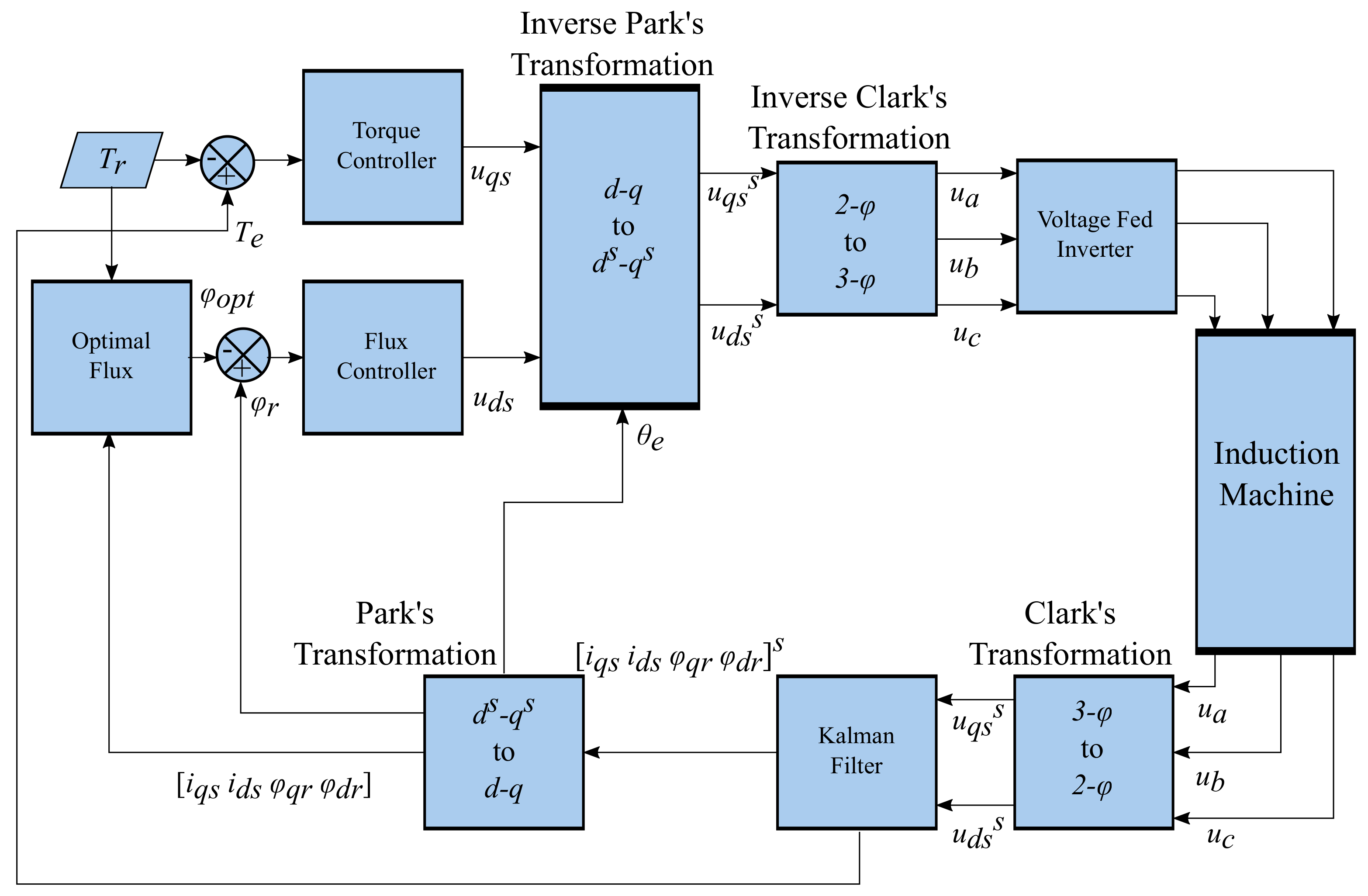
RFOC architecture for IM is presented in Figure 3. It can be seen that the design of the PI-based torque and flux controllers uses the variables in SRRF, whereas, DKF is designed by using the SRF model. The control voltages and in are converted to voltages through a series of inverse Park’s and Clarke’s transformations, respectively. Then, set of voltages , , and are fed into the inverter which eventually drives the IM. On the other hand, the set of measured stator voltages from IM are converted to and by using Clarke’s transformation (cf. (2)). Based on the measurements and input voltages, DKF estimates and by using the algorithm given in (29) and (30). Then, for the controller design, Park’s transformation (cf. (3)) is used to convert the electrical state variables into SRRF.
The most critical parameter of RFOC is , as it is used for the transformation of SRF to SRRF and vice versa. A wrong estimation of can cause the malfunctioning of RFOC.
4. Results and Discussions
The concept of AWES presented in Figure 1 is realized using MATLAB and Simulink. The nominal values of the winch and the IM model parameters used for the simulations are given in Table 1.
Some practical considerations and assumptions for the simulation of the traction phase of the AWES are listed below:
- A variable step MATLAB solver: Ode23t is used to simulate the AWES in Figure 1. The minimum and maximum step sizes used for simulation are 5 s and 50 s, respectively.
- The minimum height of the tether from where the KM is launched into the cross wind flight is m. Whereas, the power production phase is stopped when the tether length reaches its maximum value: m.
- To evaluate the robustness of the control strategy, it is assumed that the wind gusts generate a constant disturbance torque, i.e., Nm in (1). It is important to mention here that we have not used any specific dynamic model of the wind gust. The constant value for the wind gust used was the maximum value of the disturbance considered, corresponding to the simulation of the worst case scenario.
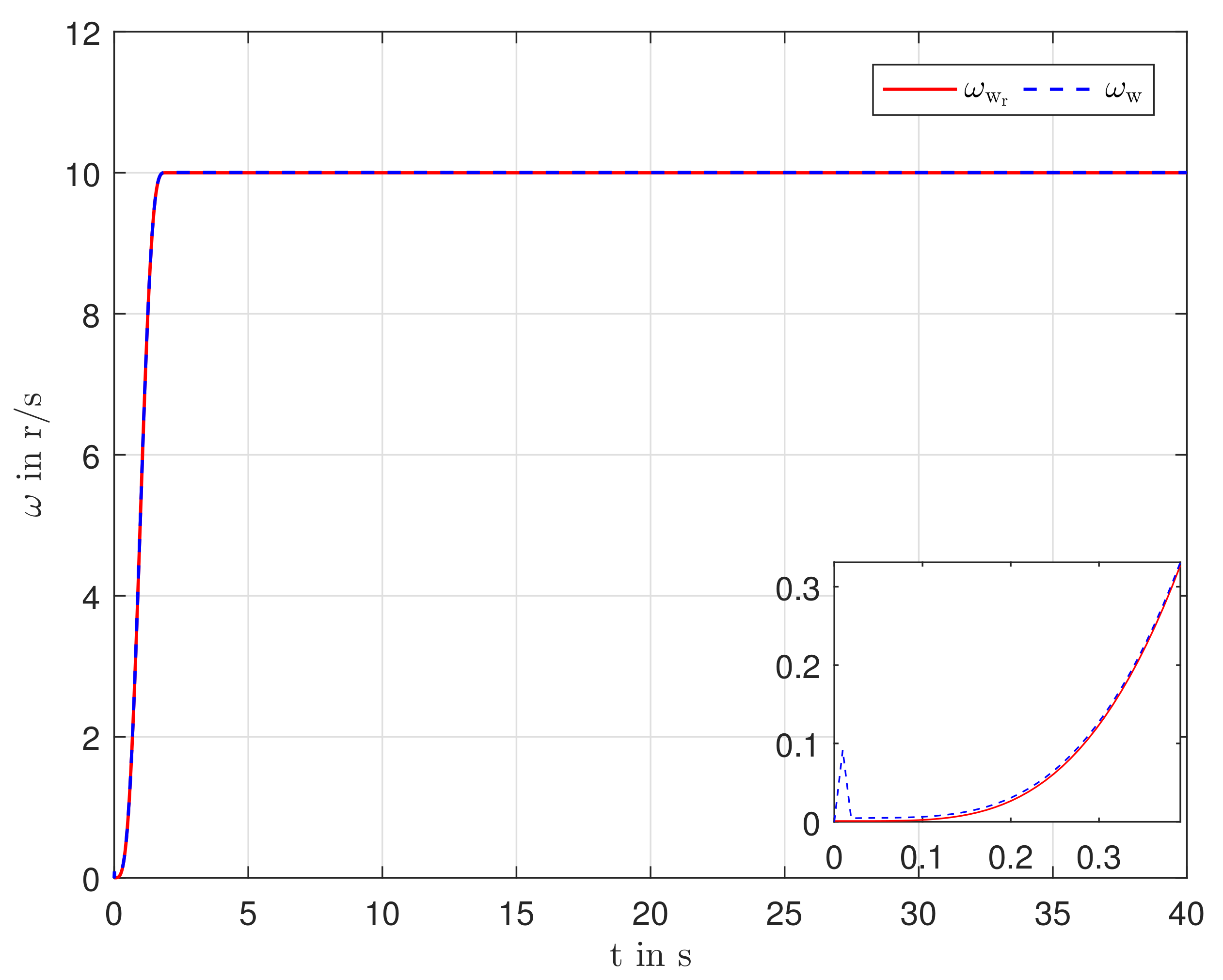
- The desired angular speed of the winch r/s for the traction pahse. Positive angular speed refers to counter-clockwise rotation, whereas, negative angular speed indicates clockwise rotation.
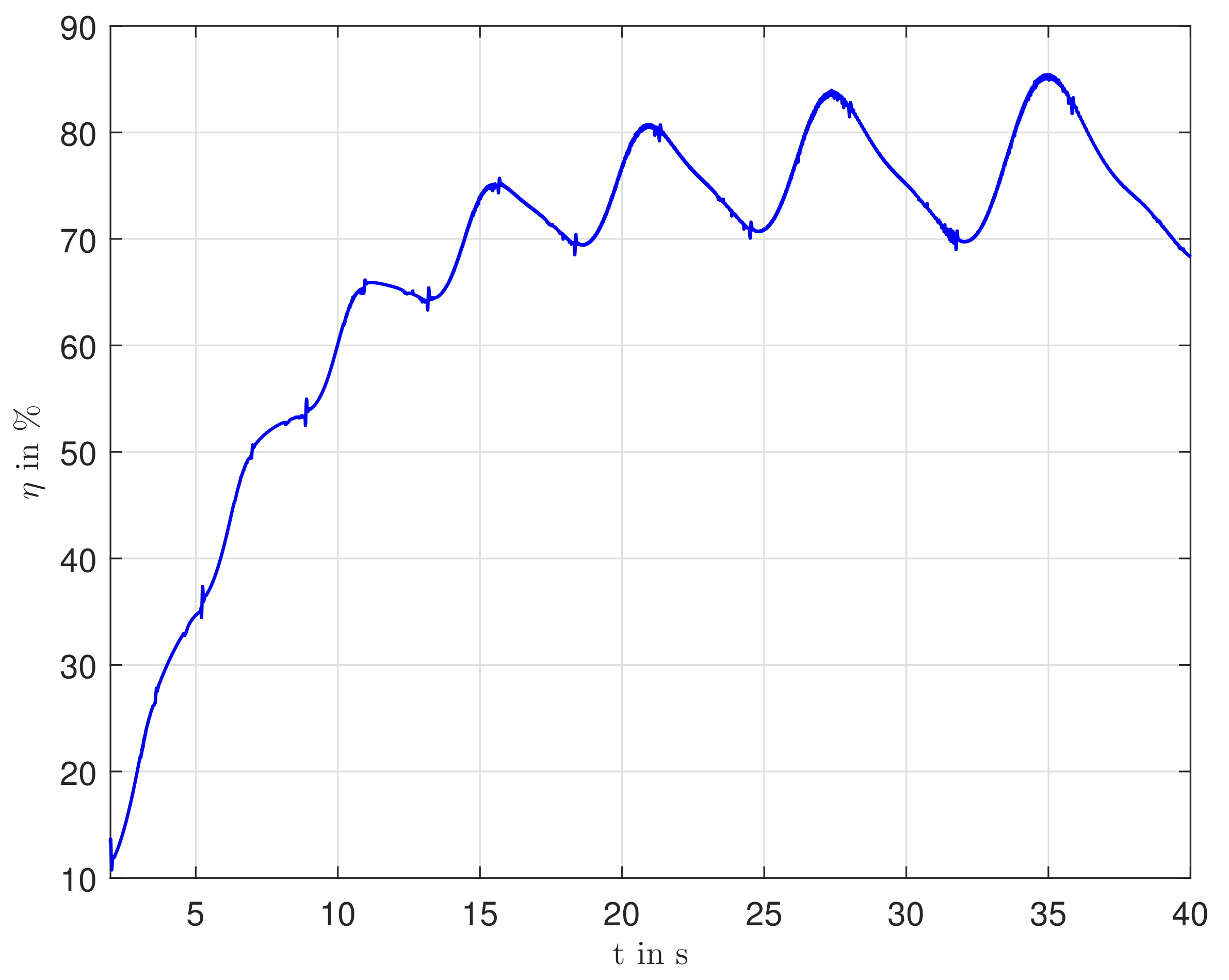
- A 5.5 KW IM with rated line-line voltage V ( V), operating at 50 Hz is considered for the simulation study. The rated speed, rated torque, and efficiency of the IM are 1461 rev/min (153 r/s), 780 Nm, and %, respectively.
- It is assumed that the gain of voltage fed inverter in Figure 2 is unity.
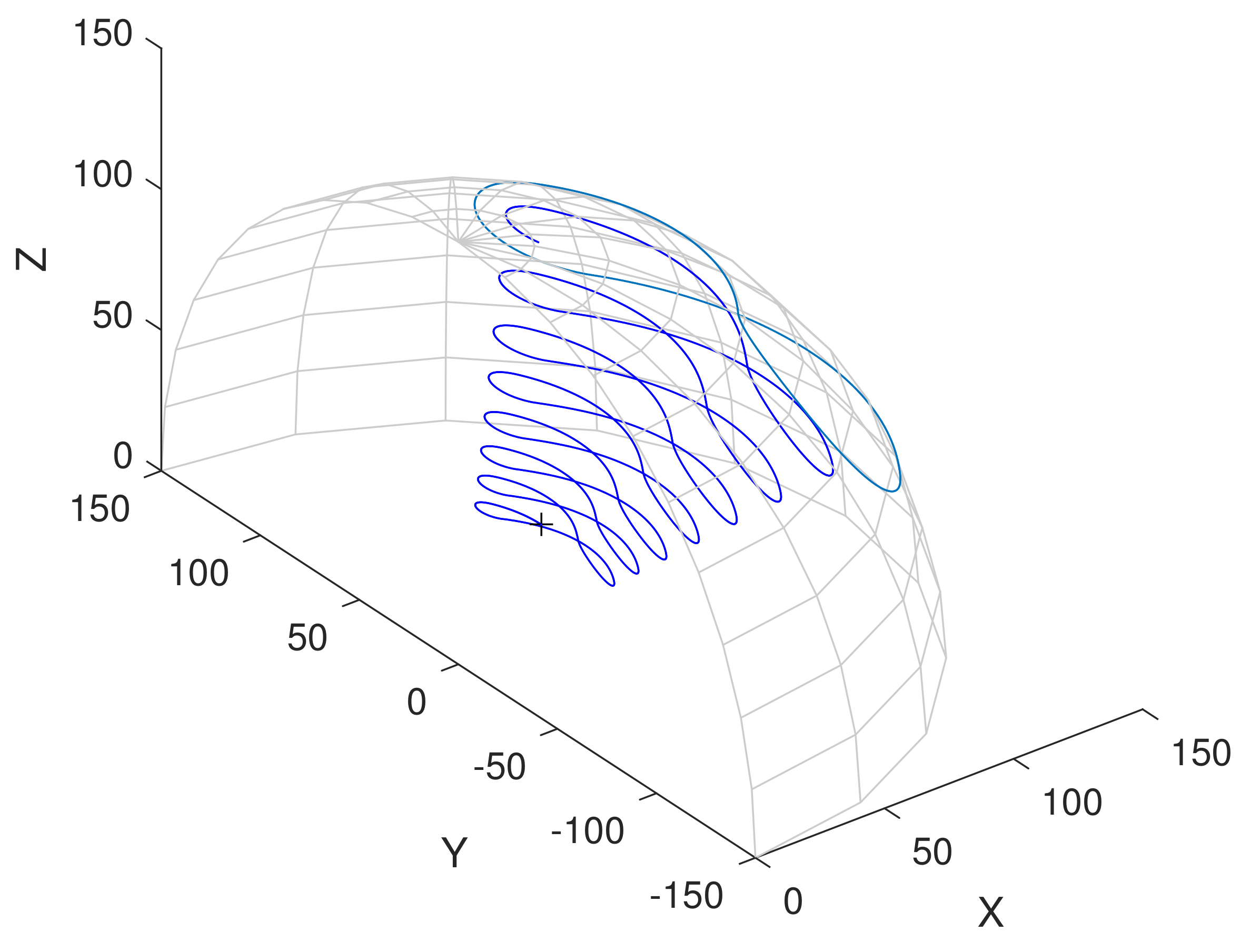
The KM of [34] is integrated with the GSM as shown in Figure 1. The orientation of the KM suitable for the traction phase is set by the local on-board controllers. During the cross-wind flight, KM pulls the tether with a large and hence the winch drives the IM, which acts as a generator to produce the electrical power. The trajectory of the KM is shown in Figure 4, which demonstrates the figure-of-eight flight trajectory.
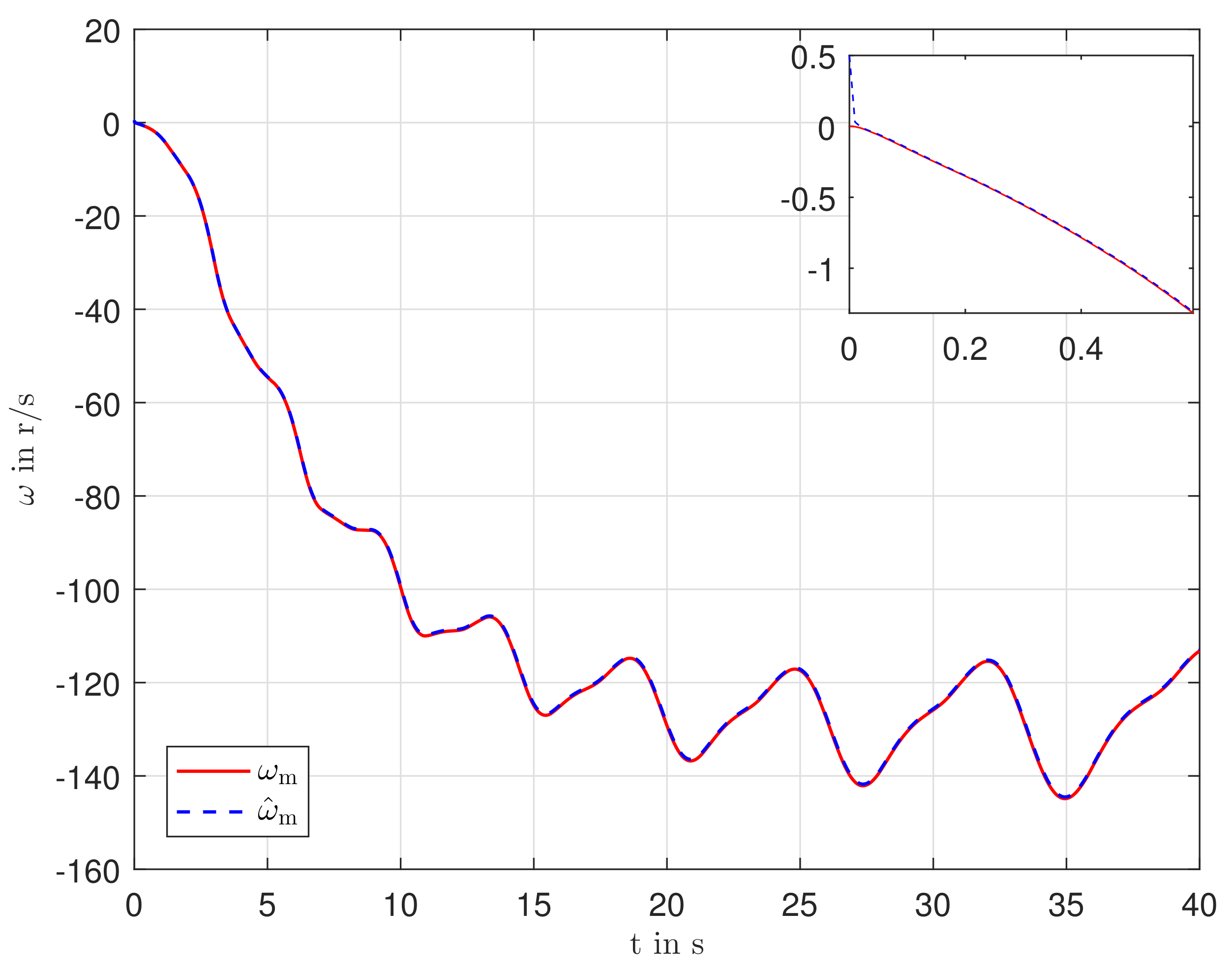
The remaining simulation results are for the cascade control of the GSM. Figure 5 shows that the winch speed controller based on SMC successfully drags to its desired level in the presence of the input disturbance . Due to the use of gears, the direction of rotation is opposite for the winch and IM. This can be seen in Figure 5 and Figure 6. The control effort for the winch speed controller is shown in Figure 7. The discontinuous gain of the SMC used for the simulations is .
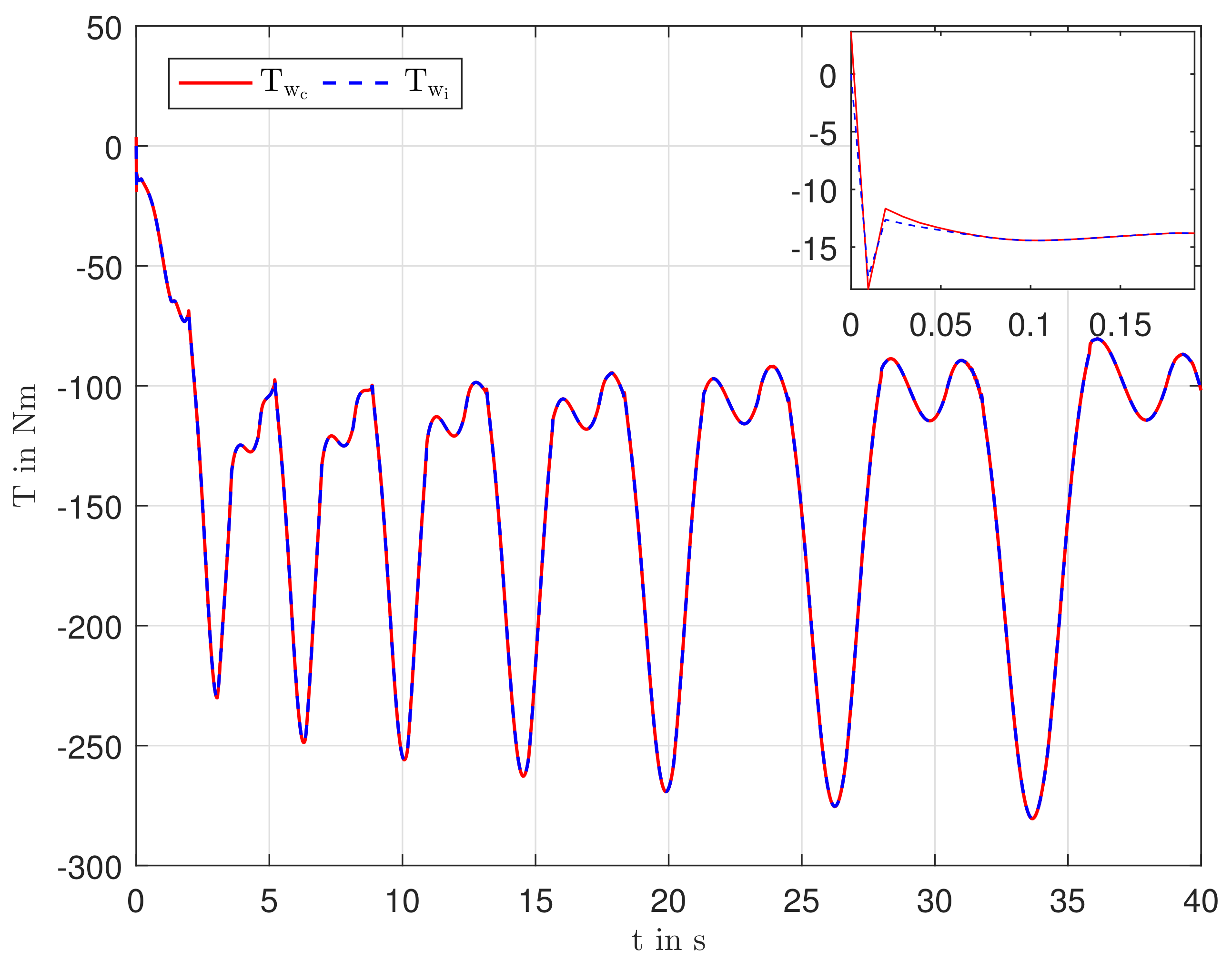
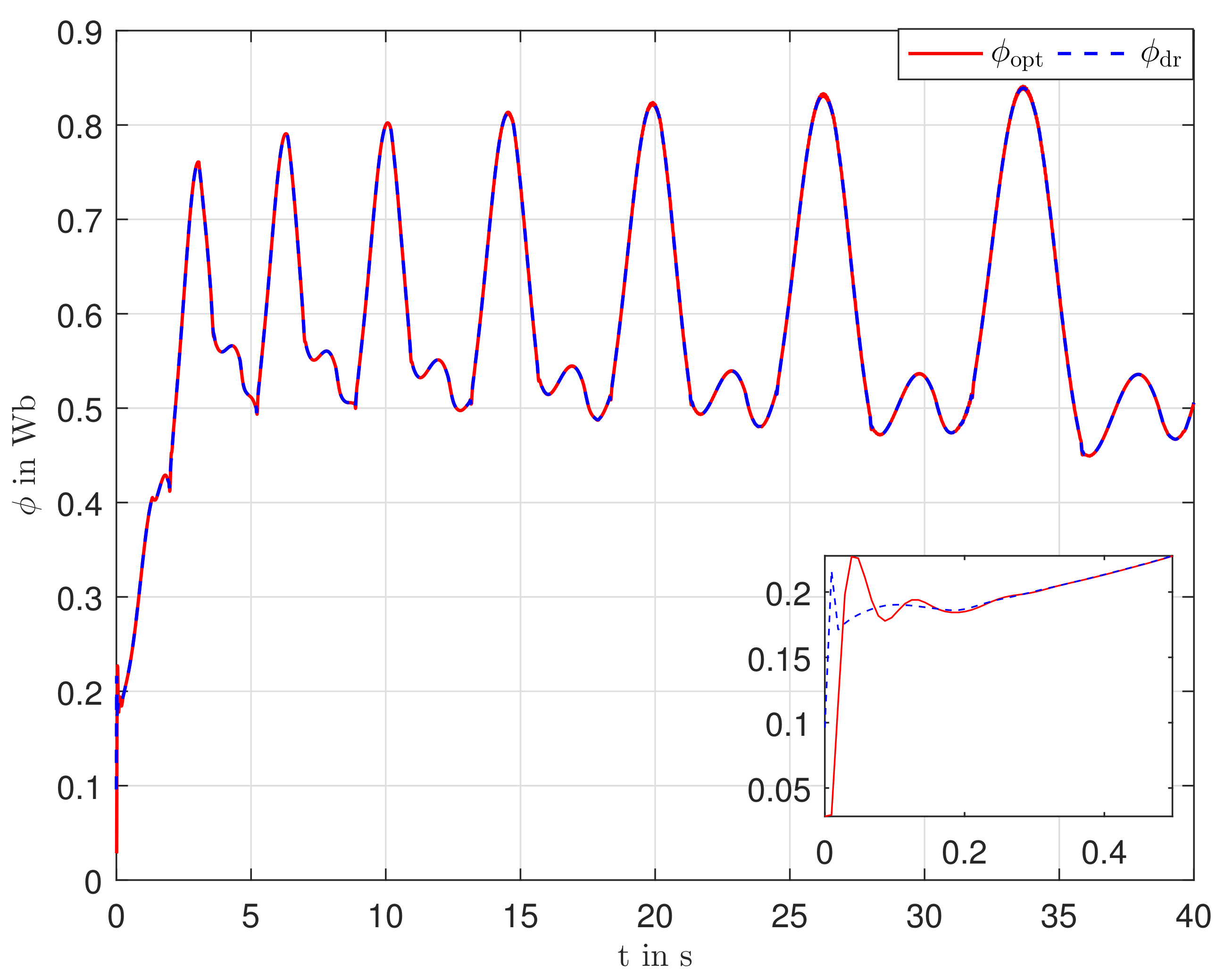
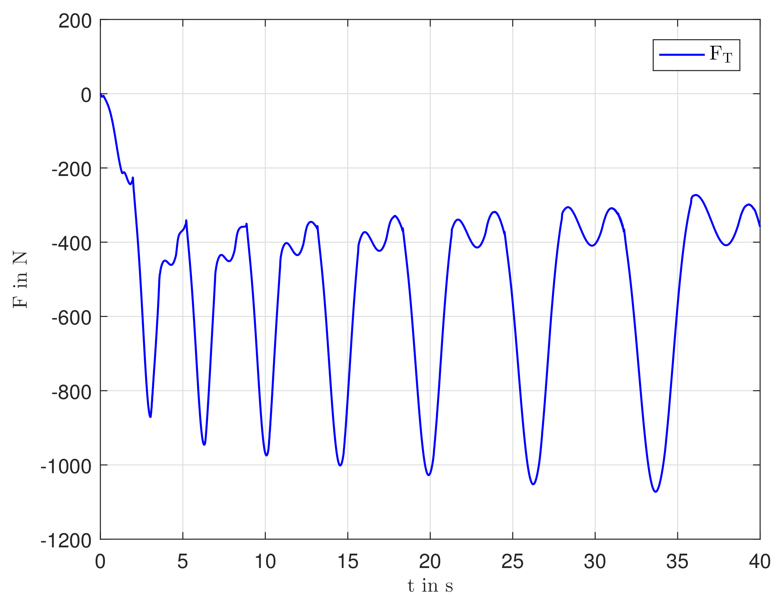
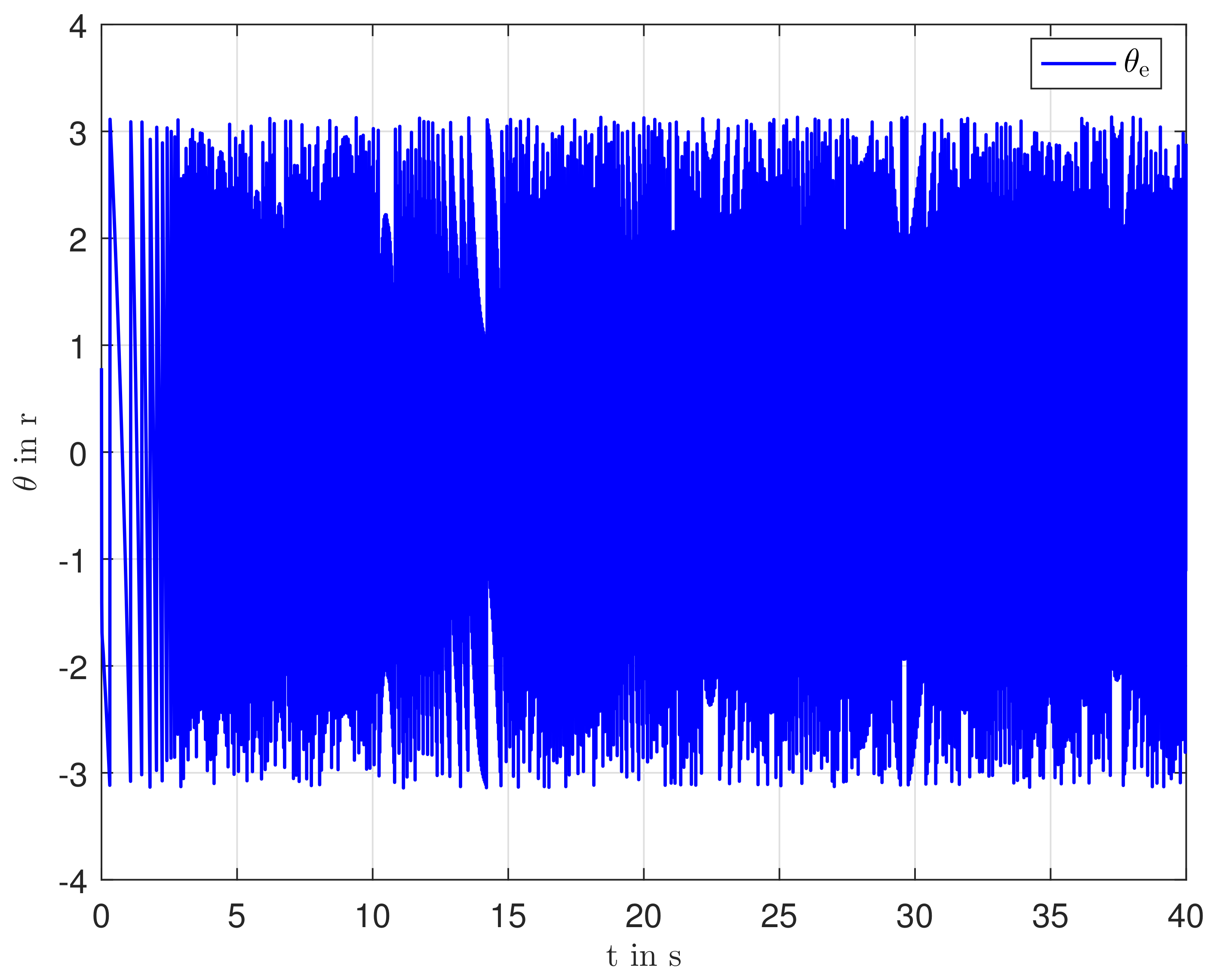
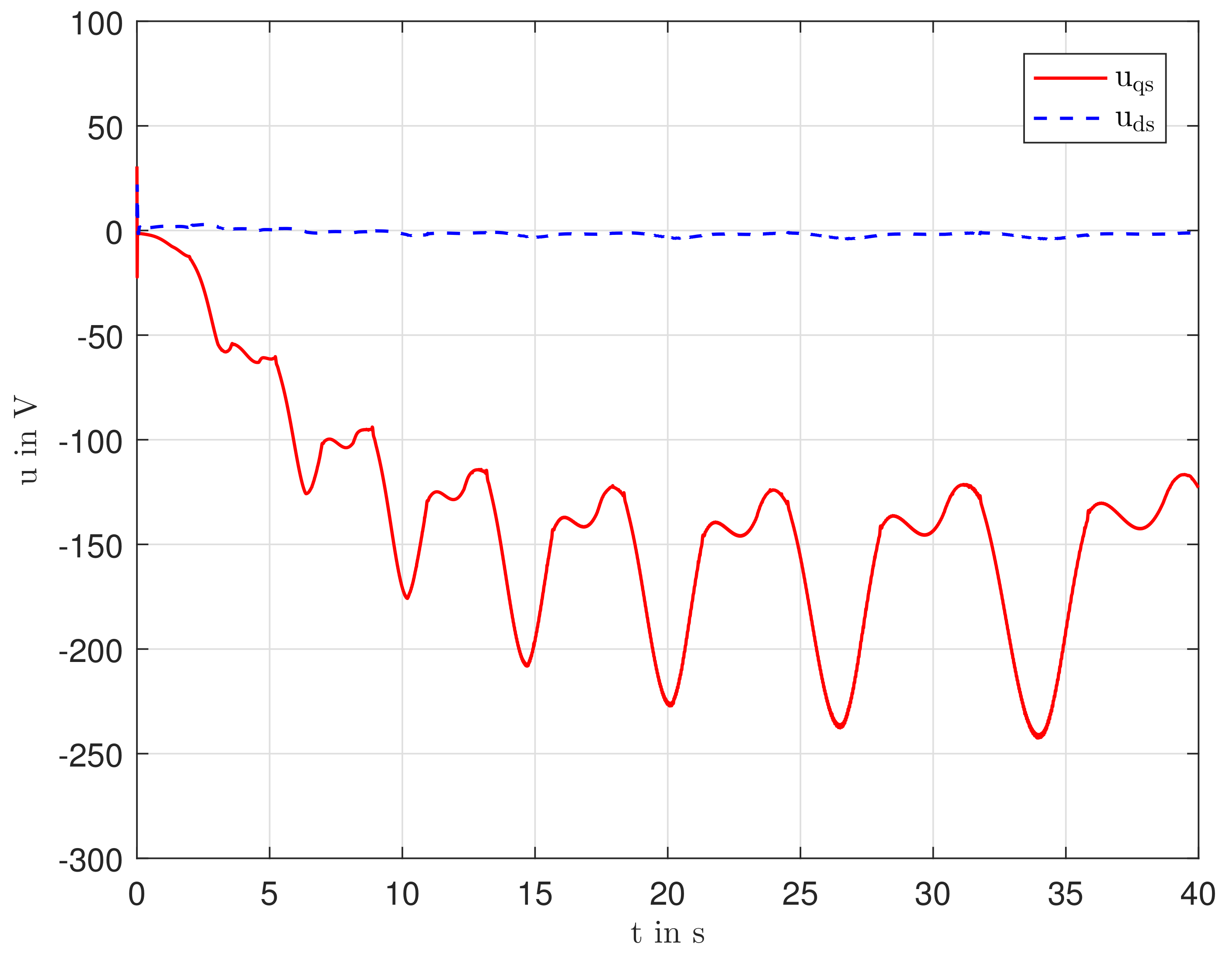
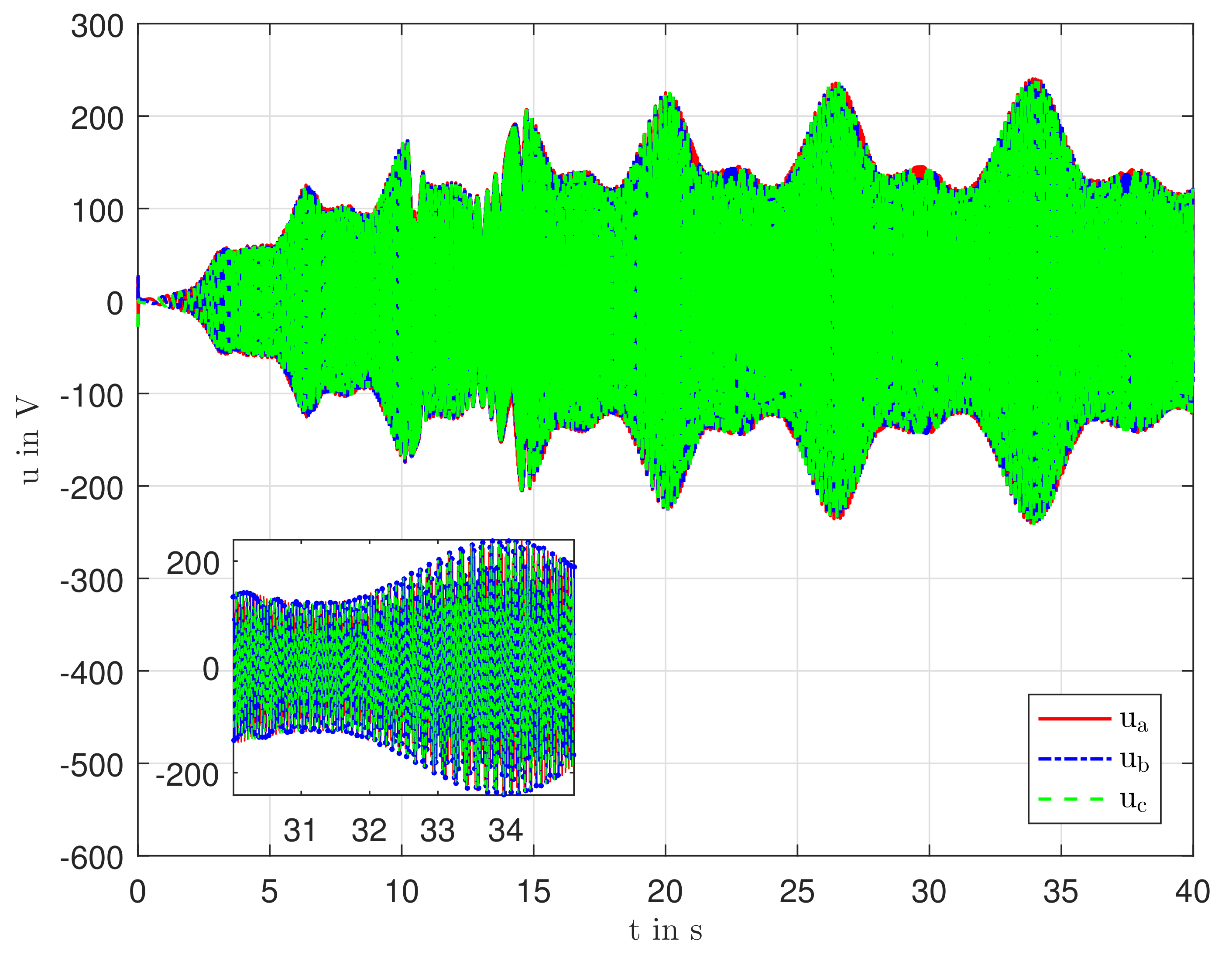
The performance of the field oriented control of the IM is demonstrated in Figure 7 and Figure 8. The tether force exerted on the winch is shown in Figure 9. During the traction phase, drives the IM, which operates as a generator to produce electricity. According to (9) and Table 1, and . Therefore, the results in Figure 7 show that the torque controller accurately keeps the induced torque of the IM to the desired level . Similarly, the rotor flux successfully tracks the optimal flux trajectory , cf. Figure 8. The electrical angle in (18), which is used for the transformation from SRF to SRRF and vice-versa is shown in Figure 10. The control voltages of the torque () and flux () PI controllers are shown in Figure 11, and the corresponding control voltages are shown in Figure 12. The proportional and integral gains for the torque and flux PI controllers are , , , and , respectively. It can be seen in Figure 7 and Figure 8, that RFOC makes the instantaneous control of both torque and flux possible.
The remaining section qualitatively evaluates the performance of the DKF, which is used to estimate and . To study the estimation behavior of the DKF, it is necessary to initialize the DKF and actual IM model with different initial conditions. Therefore, the initial conditions for the state variables of the IM model and DKF are given as:
The initial error covariance matrix in (29) is given as:
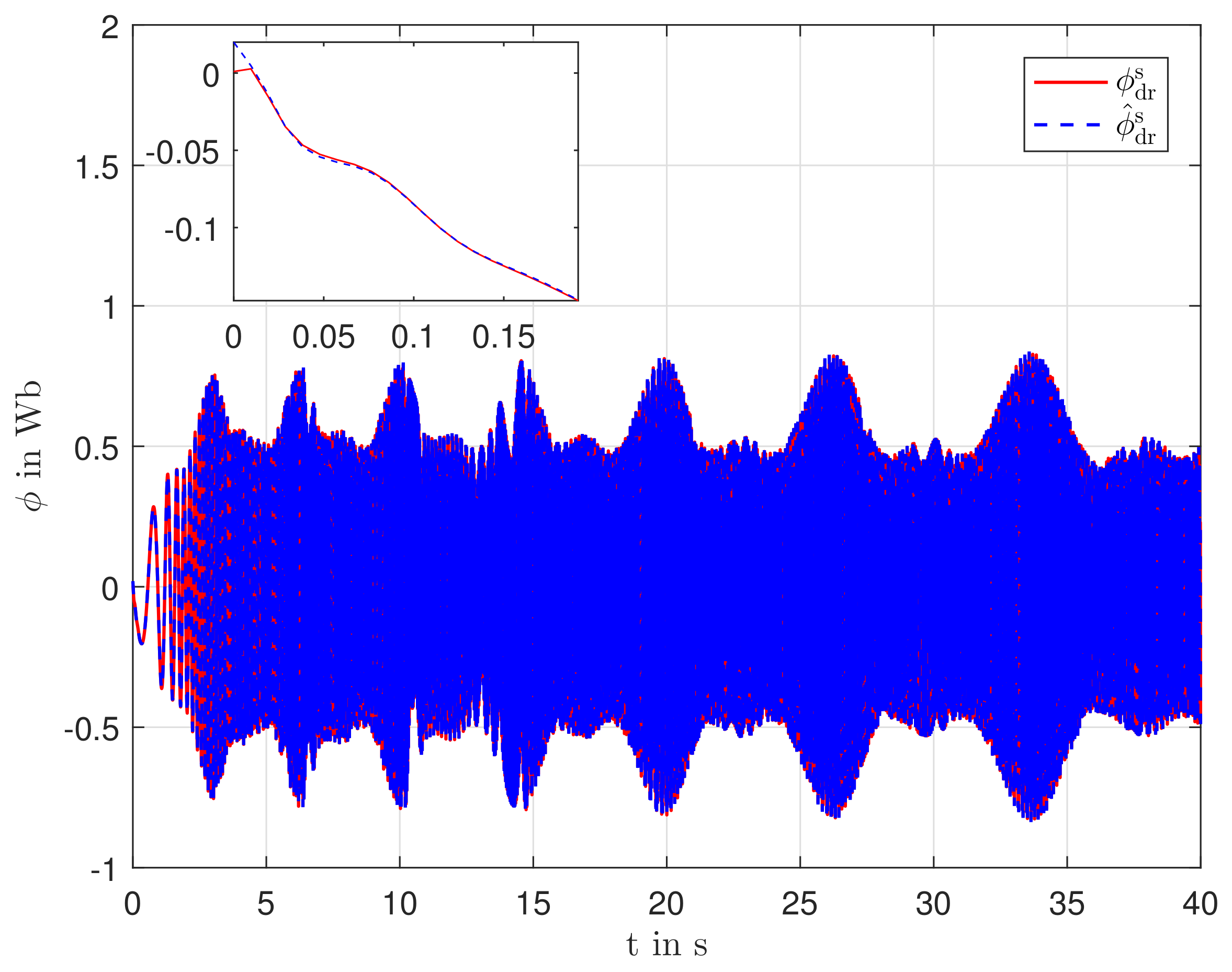
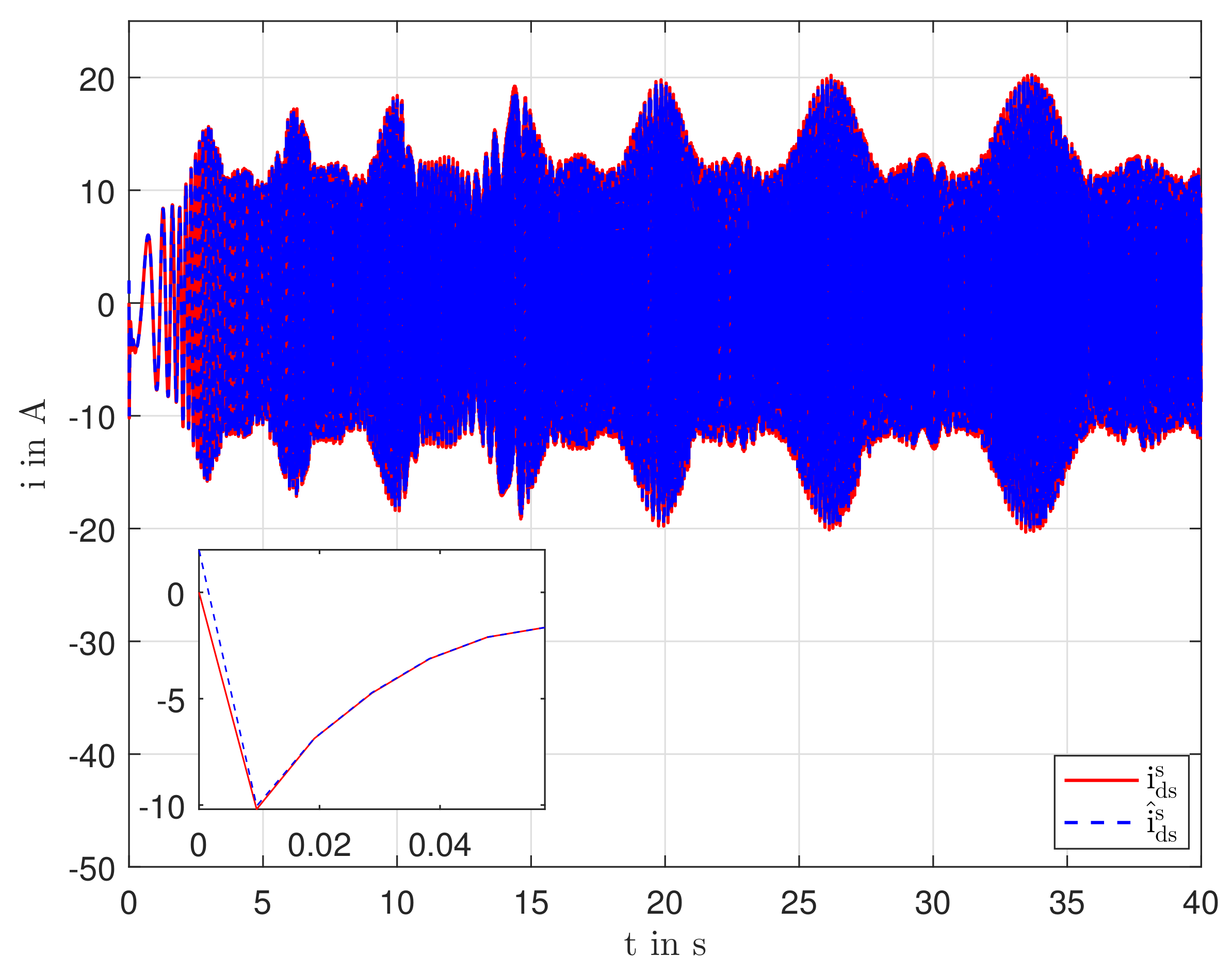
The process and measurement noises covariance matrices in (30) are selected as and , respectively. It is pertinent to mention here that the matrices Q and R are selected after a few trials. It can be seen from Figure 13 and Figure 14 that the DKF gives a very good estimate of the unknown SRF fluxes. The DKF uses speed and axes SRF currents of the IM as the measurements to reconstruct the SRF fluxes. The measured and estimated axes currents in SRF are shown in Figure 15 and Figure 16, whereas the measured and estimated IM speed is depicted in Figure 6.
Due to the varying load, the efficiency of the IM is not constant during the traction phase. The dynamic efficiency of the IM () during the traction phase is characterized as (cf. [47]):
5. Conclusions
In this paper, we consider the control architecture of an AWES and propose a controller design for one of its main modules: The ground station module (GSM). We develop a cascade control strategy for the GSM during the traction phase. The design of the cascade control system for the GSM comprises the winch speed controller in the outer loop and the torque controller of the induction machine (IM) in the inner control-loop. The integral sliding mode control (SMC) technique is used to design the winch speed controller, whereas, the IM torque control is based on rotor flux oriented control (RFOC) and is implemented with decentralized PI controllers for induced torque and for rotor flux. To enable the implementation of RFOC, a discrete Kalman filter is used to estimate the unknown states of the IM.
The performance of the proposed controllers is evaluated through simulations carried out in Matlab/Simulink. The simulator includes not only the GSM models and controllers here developed, but also known models and controllers of the KM, enabling the analysis of the overall AWES. The simulation results show that the AWES achieves the desired performance, even in the presence of external bounded disturbances, possibly representing wind gusts.
A major conclusion is that an advanced control strategy for the GSM is key for the successful operation of the overall AWES. The results presented in the paper can serve as motivation for the AWES community to provide further attention to the control of the GSM, which has been much less discussed in the literature than the control of the KM.
One of the possible future extensions of this work is the design of a robust field-oriented control for the IM, such that its performance, efficiency, and aging can be optimized during unsteady state operation. Such extension would contribute in several dimensions to the real-time implementation of the GSM control system.
Author Contributions
Conceptualization, A.A.U., F.A.C.C.F. and M.C.R.M.F.; methodology, A.A.U., F.A.C.C.F., M.C.R.M.F. and S.V.; software, A.A.U., M.C.R.M.F. and S.V.; validation, A.A.U., M.C.R.M.F. and S.V.; formal analysis, A.A.U. and M.C.R.M.F.; investigation, A.A.U., M.C.R.M.F. and S.V.; resources, A.A.U., M.C.R.M.F. and S.V.; data curation, A.A.U. and M.C.R.M.F.; writing—original draft preparation, A.A.U.; writing—review and editing, F.A.C.C.F. and M.C.R.M.F.; visualization, A.A.U. and F.A.C.C.F.; supervision, F.A.C.C.F.; project administration, F.A.C.C.F.; funding acquisition, F.A.C.C.F. All authors have read and agreed to the published version of the manuscript.
Funding
We acknowledge the support of COMPETE2020/FEDER/PT2020/POCI/MCTES/FCT funds, mainly through grant PTDC/EEI-AUT/31447/2017-UPWIND, but also grants PTDC/MAT-APL/28247/2017-ToChair, POCI-01-0145-FEDER-031821|FCT-FAST, and UID/EEA/00147/2019-SYSTEC.
Institutional Review Board Statement
Not applicable.
Informed Consent Statement
Not applicable.
Conflicts of Interest
The authors declare no conflict of interest.
Nomenclature
| , | electrical and mechanical speeds of rotor of the induction |
| machine (IM), respectively | |
| electrical angle required for field oriented control of the IM | |
| , | d and q axes rotor fluxes, respectively |
| optimal rotor flux | |
| , | d and q axes stator currents, respectively |
| , | stator and rotor resistances, respectively |
| , | stator and rotor leakage inductances, respectively |
| magnetizing inductance | |
| number of pole pairs | |
| f | frequency of stator |
| J | inertia of the IM rotor |
| b | damping coefficient of the IM rotor |
| tether tension | |
| , | desired and measured speeds of the winch |
| torque generated by winch speed controller | |
| desired and actual induced torques of the IM, respectively | |
| input torque to the winch system | |
| winch inertia | |
| damping coefficient of winch | |
| winch radius | |
| , | Number of teeth of winch and IM gears, respectively |
References
- Archer, C.L.; Caldeira, K. Global Assessment of High-Altitude Wind Power. Energies 2009, 2, 307–319. [Google Scholar] [CrossRef] [Green Version]
- Loyd, M.L. Crosswind kite power (for large-scale wind power production). J. Energy 1980, 4, 106–111. [Google Scholar] [CrossRef]
- Licitra, G.; Koenemann, J.; Bürger, A.; Williams, P.; Ruiterkamp, R.; Diehl, M. Performance assessment of a rigid wing Airborne Wind Energy pumping system. Energy 2019, 173, 569–585. [Google Scholar] [CrossRef]
- Cherubini, A.; Papini, A.; Vertechy, R.; Fontana, M. Airborne Wind Energy Systems: A review of the technologies. Renew. Sustain. Energy Rev. 2015, 51, 1461–1476. [Google Scholar] [CrossRef] [Green Version]
- Weiss, P. Airborne Wind Energy Prepares for Take Off. Engineering 2020, 6, 107–109. [Google Scholar] [CrossRef]
- Todeschini, D.; Fagiano, L.; Micheli, C.; Cattano, A. Control of a rigid wing pumping Airborne Wind Energy system in all operational phases. Control Eng. Pract. 2021, 111, 104794. [Google Scholar] [CrossRef]
- Vermillion, C.; Cobb, M.; Fagiano, L.; Leuthold, R.; Diehl, M.; Smith, R.S.; Wood, T.A.; Rapp, S.; Schmehl, R.; Olinger, D.; et al. Electricity in the air: Insights from two decades of advanced control research and experimental flight testing of airborne wind energy systems. Annu. Rev. Control 2021, in press. [Google Scholar] [CrossRef]
- Salma, V.; Friedl, F.; Schmehl, R. Improving reliability and safety of airborne wind energy systems. Wind Energy 2020, 23, 340–356. [Google Scholar] [CrossRef] [Green Version]
- Rapp, S.; Schmehl, R.; Oland, E.; Haas, T. Cascaded Pumping Cycle Control for Rigid Wing Airborne Wind Energy Systems. J. Guid. Control Dyn. 2019, 42, 2456–2473. [Google Scholar] [CrossRef]
- Jehle, C.; Schmehl, R. Applied Tracking Control for Kite Power Systems. J. Guid. Control Dyn. 2014, 37, 1211–1222. [Google Scholar] [CrossRef] [Green Version]
- Rapp, S.; Schmehl, R.; Oland, E.; Smidt, S.; Haas, T.; Meyers, J. A Modular Control Architecture for Airborne Wind Energy Systems. In Proceedings of the AIAA Scitech 2019 Forum, San Diego, CA, USA, 7–11 January 2019. [Google Scholar] [CrossRef] [Green Version]
- Wood, T.A.; Hesse, H.; Smith, R.S. Predictive Control of Autonomous Kites in Tow Test Experiments. IEEE Control Syst. Lett. 2017, 1, 110–115. [Google Scholar] [CrossRef]
- Ruiterkamp, R.; Sieberling, S. Description and Preliminary Test Results of a Six Degrees of Freedom Rigid Wing Pumping System. In Airborne Wind Energy; Ahrens, U., Diehl, M., Schmehl, R., Eds.; Springer: Berlin/Heidelberg, Germany, 2013; pp. 443–458. [Google Scholar] [CrossRef]
- Wood, T.A.; Hesse, H.; Zgraggen, A.U.; Smith, R.S. Model-based flight path planning and tracking for tethered wings. In Proceedings of the 2015 54th IEEE Conference on Decision and Control (CDC), Osaka, Japan, 15–18 December 2015; pp. 6712–6717. [Google Scholar] [CrossRef]
- Fechner, U.; Schmehl, R. Flight path control of kite power systems in a turbulent wind environment. In Proceedings of the 2016 American Control Conference (ACC), Boston, MA, USA, 6–8 July 2016; pp. 4083–4088. [Google Scholar] [CrossRef]
- Fagiano, L.; Schnez, S. On the take-off of airborne wind energy systems based on rigid wings. Renew. Energy 2017, 107, 473–488. [Google Scholar] [CrossRef] [Green Version]
- Bontekoe, E. Up! How to Launch and Retrieve a Tethered Aircraft. Master’s Thesis, Delft University of Technology, Delft, The Netherlands, 2010. [Google Scholar]
- Fagiano, L.; Nguyen-Van, E.; Rager, F.; Schnez, S.; Ohler, C. Autonomous Takeoff and Flight of a Tethered Aircraft for Airborne Wind Energy. IEEE Trans. Control Syst. Technol. 2018, 26, 151–166. [Google Scholar] [CrossRef] [Green Version]
- Rapp, S.; Schmehl, R. Vertical Takeoff and Landing of Flexible Wing Kite Power Systems. J. Guid. Control Dyn. 2018, 41, 2386–2400. [Google Scholar] [CrossRef]
- Fagiano, L.; Huynh, K.; Bamieh, B.; Khammash, M. On Sensor Fusion for Airborne Wind Energy Systems. IEEE Trans. Control Syst. Technol. 2014, 22, 930–943. [Google Scholar] [CrossRef] [Green Version]
- Girrbach, F.; Hol, J.D.; Bellusci, G.; Diehl, M. Optimization-Based Sensor Fusion of GNSS and IMU Using a Moving Horizon Approach. Sensors 2017, 17, 1159. [Google Scholar] [CrossRef] [PubMed]
- Malz, E.C.; Walter, V.; Göransson, L.; Gros, S. The value of airborne wind energy to the electricity system. Wind Energy 2021. [Google Scholar] [CrossRef]
- Fernandes, M.C.R.M.; Paiva, L.T.; Fontes, F.A.C.C. Optimal Path and Path-Following Control in Airborne Wind Energy Systems. In Advances in Evolutionary and Deterministic Methods for Design, Optimization and Control in Engineering and Sciences; Gaspar-Cunha, A., Periaux, J., Giannakoglou, K.C., Gauger, N.R., Quagliarella, D., Greiner, D., Eds.; Computational Methods in Applied Sciences; Springer International Publishing: Cham, Switzerland, 2021; pp. 409–421. [Google Scholar] [CrossRef]
- Paiva, L.T.; Fontes, F.A.C.C. Optimal electric power generation with underwater kite systems. Computing 2018, 100, 1137–1153. [Google Scholar] [CrossRef]
- Paiva, L.T.; Fontes, F.A.C.C. Optimal Control Algorithms with Adaptive Time-Mesh Refinement for Kite Power Systems. Energies 2018, 11, 475. [Google Scholar] [CrossRef] [Green Version]
- Canale, M.; Fagiano, L.; Milanese, M. High Altitude Wind Energy Generation Using Controlled Power Kites. IEEE Trans. Control Syst. Technol. 2010, 18, 279–293. [Google Scholar] [CrossRef]
- Zanon, M.; Gros, S.; Andersson, J.; Diehl, M. Airborne Wind Energy Based on Dual Airfoils. IEEE Trans. Control Syst. Technol. 2013, 21, 1215–1222. [Google Scholar] [CrossRef] [Green Version]
- Karg, B.; Lucia, S. Learning-based approximation of robust nonlinear predictive control with state estimation applied to a towing kite. In Proceedings of the 2019 18th European Control Conference (ECC), Naples, Italy, 25–28 June 2019; pp. 16–22. [Google Scholar] [CrossRef]
- Bafandeh, A.; Vermillion, C. Altitude Optimization of Airborne Wind Energy Systems via Switched Extremum Seeking—Design, Analysis, and Economic Assessment. IEEE Trans. Control Syst. Technol. 2017, 25, 2022–2033. [Google Scholar] [CrossRef]
- Zgraggen, A.U.; Fagiano, L.; Morari, M. Real-Time Optimization and Adaptation of the Crosswind Flight of Tethered Wings for Airborne Wind Energy. IEEE Trans. Control Syst. Technol. 2015, 23, 434–448. [Google Scholar] [CrossRef] [Green Version]
- Magdy Gamal Eldeeb, H. Modelling, Control and Post-Fault Operation of Dual Three-phase Drives for Airborne Wind Energy. Ph.D. Dissertation, Technische Universität München, München, Germany, 2019. [Google Scholar]
- Eldeeb, H.; Abdel-Khalik, A.S.; Hackl, C.M. Highly efficient fault-tolerant elelctrical drives for airborne wind energy systems. In Book of Abstracts of the International Airborne Wind Energy Conference (AWEC 2017); Diehl, M., Leuthold, R., Schmehl, R., Eds.; University of Freiburg|Delft University of Technology: Freiburg, Germany, 2017; pp. 75–77. [Google Scholar]
- Ebrahimi Salari, M.; Coleman, J.; Toal, D. Power Control of Direct Interconnection Technique for Airborne Wind Energy Systems. Energies 2018, 11, 3134. [Google Scholar] [CrossRef] [Green Version]
- Silva, G.B.; Paiva, L.T.; Fontes, F.A. A Path-following Guidance Method for Airborne Wind Energy Systems with Large Domain of Attraction. In Proceedings of the 2019 American Control Conference (ACC), Philadelphia, PA, USA, 10–12 July 2019; pp. 2771–2776. [Google Scholar] [CrossRef]
- Fernandes, M.C.R.M.; Vinha, S.; Paiva, L.T.; Fontes, F.A.C.C. L0 and L1 Guidance and Path–following Control for Airborne Wind Energy Systems. Energies 2021. submitted. [Google Scholar]
- Utkin, V. Variable structure systems with sliding modes. IEEE Trans. Autom. Control 1977, 22, 212–222. [Google Scholar] [CrossRef]
- Bose, B.K. AC Machines for Drivers. In Modern Power Electronics and AC Drives; Prentice-Hall Inc.: Hoboken, NJ, USA, 2002. [Google Scholar]
- Kim, S.H. Modeling of alternating current motors and reference frame theory. In Electric Motor Control; Kim, S.H., Ed.; Elsevier: Amsterdam, The Netherlands, 2017; Chapter 4; pp. 153–202. [Google Scholar] [CrossRef]
- Kim, S.H. Vector control of alternating current motors. In Electric Motor Control; Kim, S.H., Ed.; Elsevier: Amsterdam, The Netherlands, 2017; Chapter 5; pp. 203–246. [Google Scholar] [CrossRef]
- Teixeira, M.C.M.; Zak, S.H. Stabilizing controller design for uncertain nonlinear systems using fuzzy models. IEEE Trans. Fuzzy Syst. 1999, 7, 133–142. [Google Scholar] [CrossRef]
- Bose, B.K. Control and Estimation of Induction Motor Drive. In Modern Power Electronics and AC Drives; Prentice-Hall Inc.: Hoboken, NJ, USA, 2002; Chapter 8; pp. 29–97. [Google Scholar]
- Hanif, A. Electric Machine Control Design for Hybrid Electric Vehicles. Ph.D. Thesis, Capital Universiyt of Science and Technology, Islamabad, Pakistan, 2018. [Google Scholar]
- Utkin, V.; Guldner, J.; Shi, J. Introduction. In Sliding Mode Control in Electro-Mechanical Systems, 2nd ed.; CRC Press: Boca Raton, FL, USA, 2009. [Google Scholar]
- Edwards, C.; Spurgeon, S. Sliding Mode Control: Theory And Applications; CRC Press: Londo, UK, 1998. [Google Scholar] [CrossRef]
- Uppal, A.A.; Butt, S.S.; Khan, Q.; Aschemann, H. Robust tracking of the heating value in an underground coal gasification process using dynamic integral sliding mode control and a gain-scheduled modified Utkin observer. J. Process Control 2019, 73, 113–122. [Google Scholar] [CrossRef]
- Simon, D. The discrete-time Kalman filter. In Optimal State Estimation; John Wiley & Sons Ltd.: Hoboken, NJ, USA, 2006; Section 5; pp. 121–148. [Google Scholar] [CrossRef]
- Hanif, A.; Ahmed, Q.; Bhatti, A.I.; Rizzoni, G. A Unified Control Framework for Traction Machine Drive Using Linear Parameters Varying-Based Field-Oriented Control. J. Dyn. Syst. Meas. Control 2020, 142, 101006. [Google Scholar] [CrossRef]
Figure 1.
Two-loop control strategy for GSM.

Figure 2.
Rotor flux-oriented control of IM. (a) Alignment of rotor flux. (b) Rotor flux angle calculation.
Figure 2.
Rotor flux-oriented control of IM. (a) Alignment of rotor flux. (b) Rotor flux angle calculation.

Figure 3.
RFOC architecture for IM.

Figure 4.
Trajectory of the KM during traction phase.

Figure 5.
Desired and actual winch speeds.

Figure 6.
Measured and estimated IM speeds.

Figure 7.
Desired and actual winch torques.

Figure 8.
Desired and actual rotor flux.

Figure 9.
Tether force from KM.

Figure 10.
Electrical angle used for RFOC.

Figure 11.
Two-phase control voltages of IM.

Figure 12.
Three-phase control voltages of the IM.

Figure 13.
Actual and estimated axis flux of the IM.

Figure 14.
Actual and estimated axis flux of the IM.

Figure 15.
Measured and estimated axis current of the IM.

Figure 16.
Measured and estimated axis current of the IM.

Figure 17.
Dynamic efficiency of the IM during traction phase.


Table 1.
Nominal parameters of the winch and IM models.
| Parameter | Value | Parameter | Value | Parameter | Value | Parameter | Value |
|---|---|---|---|---|---|---|---|
| 2 | 0.295 | 0.379 | 0.0608 | ||||
| 0.0608 | 0.059 | J | 0.62 | b | 0.1 | ||
| 0.01 | 0.124 | 0.25 | 12 |
Publisher’s Note: MDPI stays neutral with regard to jurisdictional claims in published maps and institutional affiliations. |
© 2021 by the authors. Licensee MDPI, Basel, Switzerland. This article is an open access article distributed under the terms and conditions of the Creative Commons Attribution (CC BY) license (https://creativecommons.org/licenses/by/4.0/).
Share and Cite
MDPI and ACS Style
Uppal, A.A.; Fernandes, M.C.R.M.; Vinha, S.; Fontes, F.A.C.C. Cascade Control of the Ground Station Module of an Airborne Wind Energy System. Energies 2021, 14, 8337. https://0-doi-org.brum.beds.ac.uk/10.3390/en14248337
AMA Style
Uppal AA, Fernandes MCRM, Vinha S, Fontes FACC. Cascade Control of the Ground Station Module of an Airborne Wind Energy System. Energies. 2021; 14(24):8337. https://0-doi-org.brum.beds.ac.uk/10.3390/en14248337
Chicago/Turabian StyleUppal, Ali Arshad, Manuel C. R. M. Fernandes, Sérgio Vinha, and Fernando A. C. C. Fontes. 2021. "Cascade Control of the Ground Station Module of an Airborne Wind Energy System" Energies 14, no. 24: 8337. https://0-doi-org.brum.beds.ac.uk/10.3390/en14248337
Note that from the first issue of 2016, this journal uses article numbers instead of page numbers. See further details here.