Article

Sensitivity Analysis of 4R3C Model Parameters with Respect to Structure and Geometric Characteristics of Buildings

by
Ali Bagheri
1,
Konstantinos N. Genikomsakis
2,
Véronique Feldheim
3 and
Christos S. Ioakimidis
4,*
1
European Research Area Chair ‘Net-Zero Energy Efficiency on City Districts, NZED’ Unit, Research Institute for Energy, University of Mons, Rue de l’Epargne 56, 7000 Mons, Belgium
2
Inteligg P.C., Karaiskaki 28, 10554 Athens, Greece
3
Thermal Engineering and Combustion Unit, Rue de l’Epargne 56, University of Mons, 7000 Mons, Belgium
4
Center for Research and Technology Hellas/Hellenic Institute of Transport, CERTH/HIT), 6th Km Charilaou—Thermi Rd., Thermi, Thessaloniki, Macedonia, 57001 Hellas, Greece
*
Author to whom correspondence should be addressed.
Submission received: 18 December 2020 / Revised: 18 January 2021 / Accepted: 23 January 2021 / Published: 28 January 2021
(This article belongs to the Special Issue Building Thermal Envelope - New Trends and Applications)

Abstract

:
Data-driven models, either simplified or detailed, have been extensively used in the literature for energy assessment in buildings and districts. However, the uncertainty of the estimated parameters, especially of thermal masses in resistance–capacitance (RC) models, still remains a significant challenge, given the wide variety of buildings functionalities, typologies, structures and geometries. Therefore, the sensitivity analysis of the estimated parameters in RC models with respect to different geometric characteristics is necessary to examine the accuracy of identified models. In this work, heavy- and light-structured buildings are simulated in Transient System Simulation Tool (TRNSYS) to analyze the effects of four main geometric characteristics on the total heat demand, maximum heat power and the estimated parameters of an RC model (4R3C), namely net-floor area, windows-to-floor ratio, aspect ratio, and orientation angle. Executing more than 700 simulations in TRNSYS and comparing the outcomes with their corresponding 4R3C model shows that the thermal resistances of 4-facade building structures are estimated with good accuracy regardless of their geometric features, while the insulation level has the highest impact on the estimated parameters. Importantly, the results obtained also indicate that the 4R3C model can estimate the indoor temperature with a mean square error of less than 0.5 °C for all cases.

1. Introduction

The fact that improving the energy performance of buildings is a key factor in achieving the ambitious goal of climate-neutrality by 2050, as set out in the European Green Deal, has become more pronounced recently, given that the built environment in the European Union (EU) accounts for 40% of energy consumption and 36% of greenhouse gas emissions [1]. Interestingly, most of the energy consumed in buildings, ranging between 35% and 70%, is used for heating and cooling purposes [2]. In this context, legislation initiatives are implemented for the adoption of energy efficiency measures in the building sector by the EU member states [3], while strategies to accelerate the renovation rate of the existing building stock are launched [4]. The energy efficiency of buildings depends on the efficiency of the equipment, thermal integrity of buildings, and energy consumption behavior [5]. As a result, various engineering and research challenges for the implementation of the so-called nearly zero energy buildings as part of smart cities and districts [6,7] have received increasing attention over the years.
A reliable approximation of the energy consumption at a district level requires detailed information about the geometry and structure of buildings along with the stochastic behavior of occupants. Due to the lack of information at this level for a large number of buildings, 3D models and simulations require more meticulous input information as well as more accurate assumptions to generate reliable results [8]. On the other hand, it is shown that simple models, which consider the aggregation of wall and roof components into a limited number of orientations, can reduce the simulation costs significantly [9]. However, using merely a limited number of reference buildings for energy assessment at a district level, e.g., TABULA tables [10], can significantly under/overestimate total energy demands [9].
In this context, developing simulation techniques that can address these two main shortcomings (i.e., detailed input information and use of representative buildings) for developing district energy models is still an open research challenge [11]. Resistance–capacitance (RC) models provide an alternative approach to disaggregate complex problems into sub-problems, such as a district model into smaller parts, i.e., buildings. RC models have been employed in various energy assessment problems in buildings [12], either as simple models with few parameters or complicated structures with tens of resistances and capacitances [13]. Specifically, the application of a simplified RC network for estimating the thermal load of a typical office building is studied by Ogunsola and Song [14]. Harb et al. [15] examines first, second, and third order RC models for forecasting the thermal response of three buildings of different size and type. Thomas et al. [16] employed a simplified RC model for predicting the thermal performance of an office building as part of an energy management system in a microgrid based on mixed integer linear programming (MILP), in order to meet the thermal comfort needs of the occupants. In the same framework, Mugnini et al. [17] combine an RC thermal network with model predictive control (MPC) to minimize the total cost for meeting the thermal demand requirements in a building. The trade-off between reduction of model complexity in RC networks and accuracy of energy prediction in residential building simulation is discussed by De Rosa et al. [18].
As already pointed out, energy assessment at a district level requires more attention due to various buildings geometries and structures in a district, implying that a proper assessment of energy consumption in a building or district should take into account ingeniously the geometric characteristics of the envelopes and structures. Although a large body of the literature describes various data-driven models for buildings and districts [19,20,21], it is still unclear how accurately data-driven models, especially RC models, represent the thermal properties of a building when geometric characteristics change from one building to another. To address this open research problem and fill-in the relevant gap in the literature, the present work examines the variations of the total heat demand and maximum heat power in buildings due to different building structures and geometries. Furthermore, a sensitivity analysis of the estimated parameters of an RC model with respect to different geometric characteristics is conducted for expanding the application of RC models with a clearer perception about the variation of the parameters in larger models used for small neighborhoods or districts.
In this work, the estimated parameters in an RC model are compared with the thermal properties of the building structure. The application of such a study can pave the way for more complex structures and systems of different size. It is emphasized that the study presented in this paper is particularly important at the early stage of the design process, where rather limited datasets are available to generate data-driven models. Furthermore, this approach serves as the basis for analyzing larger formations of buildings, as in the case of smart neighborhoods and smart districts. Therefore, expanding such an analysis for various climate conditions while considering other type of buildings with different functionalities can be the first step to generate thermal network models of buildings in smart cities, however, this is beyond the scope of the present paper.
For the purposes of this work, a Transient System Simulation Tool (TRNSYS)-based dataset for heavy- and light-structured 4-façade buildings is developed. The values of 4 geometric characteristics, namely surface area (SA), aspect ratio (AR), windows-to-floor ratio (WF) and orientation angle (OA), change in each iteration of the TRNSYS simulations in order to cover a large variety of conditions. Using system identification techniques, the corresponding RC models, with 4 resistances and 3 capacitances (4R3C), for each simulated building in TRNSYS are generated. The variations in the total heat demand and maximum heat power of the TRNSYS models are studied to find out the geometric characteristic that has the largest effect on the energy demand in buildings. Furthermore, the estimated parameters in the 4R3C model are compared with their calculated values in TRNSYS and their deviation is studied to identify how, and which parameters are mostly affected due to the changes in the geometry of a building.
The rest of the paper is structured as follows: Section 2 describes the methods for modelling heavy- and light-structured buildings in TRNSYS considering their properties and geometric characteristics, as well as presents in detail the development of the RC model along with the system identification approach employed. Section 3 presents the results obtained from the TRNSYS simulations and RC models, provides an analytic comparison between both approaches and discusses the sensitivity analysis of the model parameters. Last, Section 4 underlines the main findings of this work and concludes the paper.

2. Materials and Methods

2.1. Heavy- and Light-Structured Building Simulation in TRNSYS

The sensitivity of estimated parameters in an RC model for predicting the heat demand will be analyzed with respect to the structure of a building, its geometric characteristics and insulation level. Heavy- and light-structured 4-facade buildings are thus simulated in TRNSYS for the purposes of this work, using the surface area, aspect ratio, windows-to-floor surface ratio, and orientation angle as geometric characteristics due to their large effect on the received solar gains. Moreover, the different insulation levels are studied to understand how retrofitting in buildings can alter the parameters in a developed RC model.

2.1.1. Structure Properties of Roof, Floor, Walls, and Windows

The simulated buildings in TRNSYS are detached buildings and the construction materials are extracted from the TABULA WebTool [22] for heavy- and light-structured buildings. The simulated buildings have a flat roof which is made of 15 cm of mineral wool and 2 cm of wood, with the properties shown in Table 1.
The U-value of different parts of the structure can be calculated from the thermal properties of the multi-layer series-resistance. For instance, the convection and radiation heat transfer on both surfaces of a wall is taken into account by adding the internal and external heat transfer coefficients to the thermal resistance of the multi-layer wall in order to calculate the overall U-value, as given in Equation (1), where Ui and Ue are the heat transmittance coefficients on internal and external surfaces respectively, t is the thickness of each layer, K is the thermal conductivity of each layer, and n is the total number of layers in a multi-layer structure.
U = ( 1 U i + l = 1 n t l K l + 1 U e ) 1
It is assumed that the heat transfer coefficients on internal and external surfaces of the roof (Ui and Ue) are 10 W/m2K and 23 W/m2K (for outdoor wind speed of 3.3 m/s) respectively [23]. Thus, the total U-value (thermal transmittance) of the roof is 0.274 W/m2K. The floor structure is also assumed to be similar in both heavy- and light-structured buildings, consisting of four layers with the properties presented in Table 2 and a total U-value of 0.177 W/m2K.
The main differences between heavy- and light-structured buildings stem from the construction materials of the walls. A heavy-structured wall is assumed to be constructed of 20 cm concrete blocks and 16 cm polystyrene for insulation, with total U-value of 0.222 W/m2K, solar absorption coefficient of 0.6 and thermal capacitance of 51.11 Wh/m2K. The thermal capacitance of the building structure corresponds to the effective thermal capacitance of a building: the thermal capacitance of walls, roof, and floor are approximated as the thermal capacitance of the structure material considered from the internal surface up to the first insulation layer only if the internal layers are massive.
This approach therefore states that the thermal capacitance of the materials after the first insulation layer does not play a significant role in the thermal capacitance of the building.
The light-structured walls are assumed to be constructed of composite and glass wool, with U-value of 0.385 W/m2K, solar absorption coefficient of 0.6, and thermal capacitance of 3.83 Wh/m2K. More detailed structure properties of heavy- and light-structured walls are presented in Table 3 and Table 4 respectively. In addition, the windows are assumed to be double glazed with a U-value of 1.1 W/m2K, the solar transmission coefficient is 0.609, and 30% of windows area is allocated for the frame which has a U-value of 1.8 W/m2K.
To analyze the effects of insulation level on the estimated parameters of an RC model, it is also assumed that the insulation material of the building envelope is polyurethane with the physical characteristics shown in Table 5. The thickness of this insulation layer changes from 0 cm (uninsulated building) to 20 cm, evenly on the entire opaque parts of the envelope, which facilitates to express the U-value of the wall and roof as a function of the insulation thickness. With these considerations, various components of heavy- and light-structured buildings are developed in TRNSYS and defining the geometric characteristics of each building is the next step to prepare the TRNSYS database for the sensitivity analysis.

2.1.2. Geometric Characteristics of Simulated Buildings

In this paper, four main indicators are identified to describe the geometric characteristic of each simulated building in TRNSYS. Each sample building can be addressed with a label such as α-β-γ-δ, where:
  • α: corresponds to the building’s floor surface area [m2], denoted as SA
  • β: corresponds to the building’s aspect ratio [unitless], denoted as AR
  • γ: corresponds to the building’s windows-to-floor surface ratio [%], denoted as WF
  • δ: corresponds to the building’s orientation angle [°], denoted OA.
The simulated buildings are single-floor 4-facade buildings that have a height of 3 m, the roof is flat, and they are all detached. Additionally, the windows are placed on the three out of four external walls. Considering the first simulated building has the largest windows area on its south wall, then east and west walls are two sidewalls where other windows are placed on. There is no window on the north wall, since the small part of solar radiation entering through northern windows renders them impractical from an architecture point of view. Figure 1 graphically represents a 100 m2 building with an aspect ratio equal to 2, windows-to-floor surface ratio of 15% and orientation angle of 0° (south orientation of the front wall).
The buildings are simulated in TRNSYS by changing the previously mentioned four characteristics (α-β-γ-δ). Specifically, it is assumed that the surface area (α parameter or SA) takes the values 50, 75, 100, 150, and 200 m2 for covering a wide range of buildings in a district. The second factor considered in this work, i.e., the aspect ratio (β parameter or AR), varies from 0.25 to 4 in the simulations. Figure 2 and Table 6 represent the aspect ratio effects on the area of walls in different buildings. The third factor is the windows-to-floor surface ratio (γ parameter or WF) which ranges from 5% to 30% in this work, having a large effect on solar gains. The calculated windows surface in each case for a 100 m2 building is given in Table 7. The last geometric factor considered in this study is the orientation angle (δ parameter or OA) which shows the angular deviation from 0° (south orientation) to 180° (north orientation). The combinations of these geometric and structural characteristics result in a total of 700 building simulations in TRNSYS. Next, the total heat demand and maximum heat power can be calculated according to the various scenarios for the indoor conditions, where controlled indoor temperature or controlled heat input can be considered [24,25].

2.1.3. Indoor Conditions and Heat Gains

The energy demand of a building depends significantly on the indoor and outdoor conditions. In this work, it is assumed that all buildings have similar set point temperature as well as similar geographical situation. Therefore, the energy consumption varies from a building to another according to their differences in structure and geometric characteristics.
It is also assumed that the simulated buildings in TRNSYS perform between two set point temperatures. The indoor temperature is set at 22 °C for working days (Monday to Friday) and working hours (8 am to 6 pm), while for the rest of the time, the minimum allowed indoor temperature is set at 15 °C, representing the temperature conditions in a hypothetical office building, in accordance to the ASHRAE standards for comfort conditions during winter [23]. It is further assumed that there is no heat recovery system, and the ventilation occurs directly between the indoor and ambient air. When the indoor temperature is set at 22 °C, the ventilation rate is 3 ach (air change per hour) and for the rest of the time it is assumed to be 0.25 ach. Moreover, the infiltration rate is assumed to be fixed at 0.24 per hour. Under these conditions, the heat transfer rate via the ventilation and infiltration can be determined from Equations (2) and (3), where ρ is the air density, cp is the specific heat of the air, V is the volume of the building, while Tin and Tout are indoor and outdoor temperatures, respectively.
Q ˙ v e n t = ρ c p V ( T i n T o u t ) × a c h 3600
Q ˙ i n f = ρ c p × 0.24 × V ( T i n T o u t ) / 3600
The Uccle meteonorm library in TRNSYS provides weather data for the simulations. In model type 56 in TRNSYS, the determined solar radiation on each surface is treated separately. The ambient temperature (Tout) is extracted directly from TRNSYS and the ground temperature Tg is fixed at 10 °C. In this work, the total solar radiation is given by Equation (4) and it is equal to the sum of the solar radiation on each surface according to their orientation angles and inclinations. More specifically, the part of the solar radiation that heats the opaque part of a building ( Q ˙ r a d 1 ) includes the solar radiation on the roof and the opaque walls as shown in Equation (5), and the part of the solar radiation that passes through windows and transparent elements enters the building ( Q ˙ r a d 2 ) and can be calculated by Equation (6), where A is the surface area, Q ˙ is the solar radiation on each surface, SC is the solar absorption/transmission coefficient, and φ is the windows to wall ratio on each surface, while the subscripts w, r, and g refer to the wall, roof and glazing respectively. Last, it is assumed that there exists no limit on the heating system and it supplies heat such as the building reaches the set point temperature during the working hours.
Q ˙ t o t a l = i = 1 4 A w i Q ˙ w i + A r Q ˙ r
Q ˙ r a d 1 = i = 1 4 S C w i A w i ( 1 φ w i ) Q ˙ w i + S C r A r Q ˙ r
Q ˙ r a d 2 = i = 1 4 S C g i A w i φ w i Q ˙ w i

2.2. Development of RC Model

RC models are developed from the lumped capacitance assumption which considers a uniform temperature distribution in the thermal mass. By this assumption, a building can be represented with a finite number of nodes which are connected to thermal capacitances (C). The heat transfer between two nodes occurs through a thermal resistance (R). Recognizing the small range of temperature variations in a building, it is possible to assume thermal resistances and capacitances to be independent of temperature changes. Therefore, a set of linear differential equations can represent various heat transfer rates in an RC model [23].
The parameters of an RC model can be determined in two approaches: (i) by the calculation from the thermal properties of the material of the structure, which is known as white-box model approach, and (ii) by the estimation from measured/simulated dataset that includes the inputs and outputs of the system, which is typically referred to as grey-box model approach. In this work, 4R3C parameters are estimated from datasets generated in TRNSYS, therefore the generated RC models are categorized as grey-box models.
In this paper, an RC model with 4 thermal resistances and 3 thermal capacitances is developed to represent the heat transfer rate between the indoor node (Tin), ambient and the ground. Fraisse et al. [26] have shown that a model with a limited number of resistances and capacitances is sufficiently accurate to represent different elements of a building. In this work, a 2R1C branch (R1, R3, and C2) is used for the building envelope and another 2R1C branch (R2, R4, and C3) for the floor structure, as shown in Figure 3. The nodes T1 and T3 are the envelope and floor temperatures respectively. Accordingly, Q ˙ v e n t , Q ˙ i n f , and Q ˙ h e a t are inserted directly into node Tin, Q ˙ r a d 1 is introduced in node T2 and Q ˙ r a d 2 is an input to node T3.
Applying the Kirchhoff’s law to the nodes in Figure 3 and using the Euler’s discretization method, the state space equations for this 4R3C model are given in Equations (7) and (8). In this formulation, the nodes Tin, T2, and T3 are the states of the system, and Tout, Tg, Q ˙ r a d 1 , Q ˙ r a d 2 , Q ˙ v e n t , Q ˙ i n f , and Q ˙ h e a t are inputs, while ∆t is the time step of the data set, and k is the discrete-time indicator.
( T i n T 2 T 3 ) ( k + 1 ) = ( 1 t R 1 C 1 t R 2 C 1 t R 1 C 1 t R 2 C 1 t R 1 C 2 1 t R 1 C 2 t R 3 C 2 0 t R 2 C 3 0 1 t R 2 C 3 t R 4 C 3 ) ( T i n T 2 T 3 ) ( k ) + ( 0 0 0 0 t C 1 t C 1 t C 1 t R 3 C 2 0 t C 2 0 0 0 0 0 t R 4 C 3 0 t C 3 0 0 0 0 ) ( T o u t T g Q ˙ r a d 1 Q ˙ r a d 2 Q ˙ v e n t Q ˙ i n f Q ˙ h e a t ) ( k )
T i n ( k ) = ( 1 0 0 ) ( T i n T 2 T 3 ) ( k ) + ( 0 0 0 0 0 0 0 ) ( T o u t T g Q ˙ r a d 1 Q ˙ r a d 2 Q ˙ v e n t Q ˙ i n f Q ˙ h e a t ) ( k )
The assigned parameters in the RC model are estimated by minimizing the mean square error (MSE) function, as shown in Equation (9), between the TRNSYS outputs for the indoor temperature and the outputs of the RC model. For this purpose, the system identification toolbox in MATLAB is utilized, which performs error minimization through Gauss-Newton, adaptive Gauss-Newton, steepest descent least square and Levenberg–Marquardt algorithms [27]. In this work, an MSE value of less than 0.5 °C is considered sufficiently accurate, corresponding to a FitPercent value greater than 80%, where FitPercent is the cost function in Equation (10). In Equation (9), N is the number of observations, which is equal to the length of the dataset, e is the calculated error between TRNSYS and RC models outputs, θ is the parameters vector consisting of R1, R2, R3, R4, C1, C2, and C3, and t is the time index.
V ( θ ) = 1 N t = 1 N e T ( θ , t ) e ( θ , t )
F i t P e r c e n t = 100 × ( 1 ( T i n T R N S Y S T R C ) 2 ( T i n T R N S Y S T i n T R N S Y S ¯ ) 2 )

3. Results and Discussion

First, the thermal performance behavior of buildings is studied with respect to the structure and geometric characteristics by simulating the first 1000 h of the typical meteorological year (TMY). Such a study provides a useful insight into the main geometric features and their impacts on the total heat demand and maximum heat power during this period. Next, a comparison is performed between the estimated parameters in the 4R3C model and their corresponding values from TRNSYS. The comparison analysis is essential in order to identify the consistent parameters, i.e., the ones that can be estimated with high accuracy, when the building’s geometry changes from one type to another. Last, the effects of insulation level on the estimated parameters of a heavy-structured building are examined to understand how the parameters in a model vary due to retrofitting in buildings.

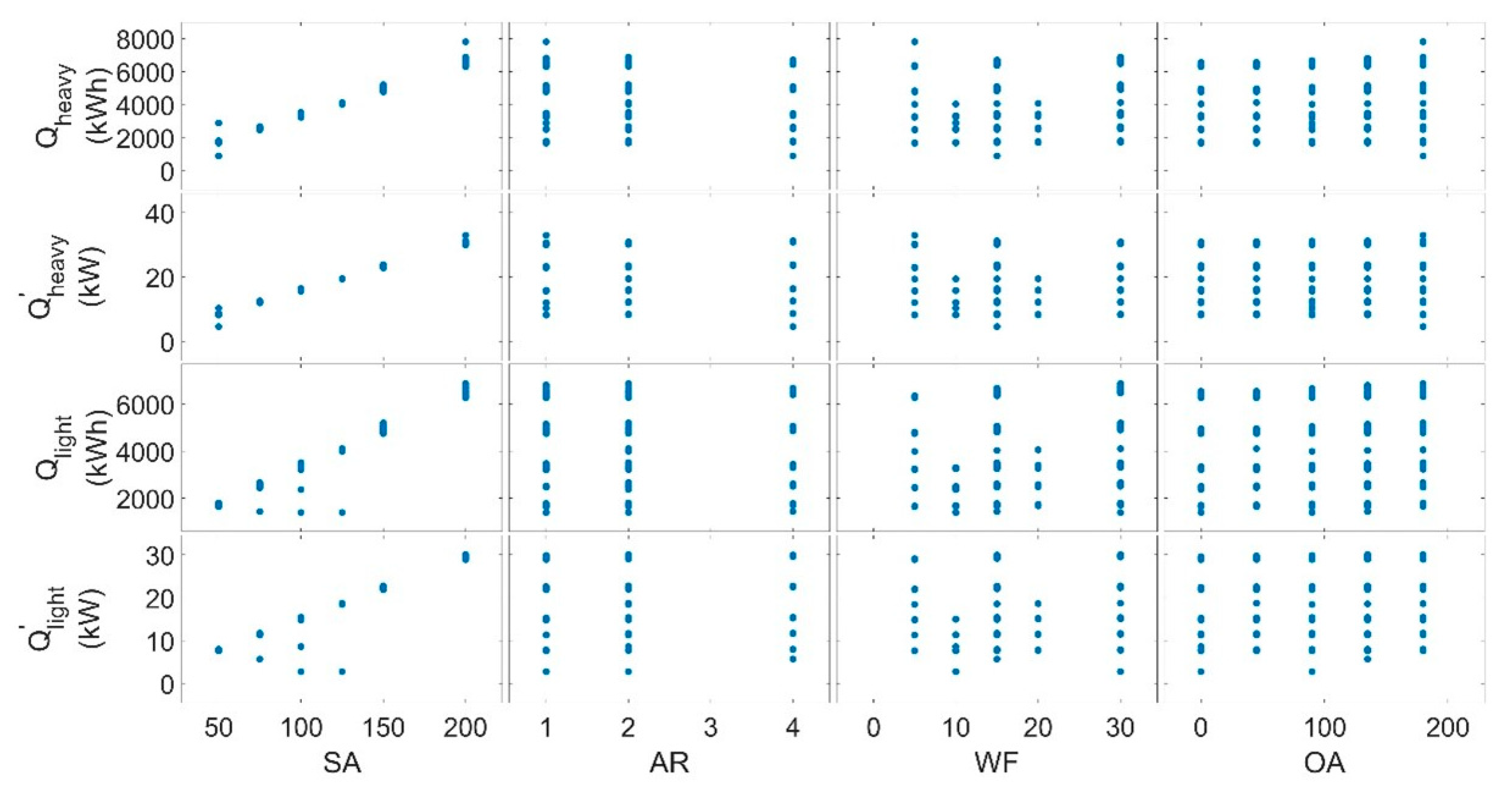
3.1. Sensitivity Analysis of Heat Consumption in Heavy- and Light-Structured Buildings with Respect to Their Geometric Characteristics

For each simulated building in TRNSYS, the ambient temperature and solar radiations are inserted from the weather database in TRNSYS for Uccle in Belgium. With respect to TMY data for Belgium, the average temperature is 9.73 °C, while the maximum and minimum temperatures are 29.7 °C and −7.9 °C respectively. In addition, for the first 1000 h the average temperature is 2.2 °C and the maximum temperature does not exceed 11.2 °C. The heat power and heat losses through ventilation and infiltration are calculated. As shown in Figure 4, for the controlled indoor temperature with the set points at 22 °C and 15 °C of a 100 m2 south-faced building with the AR value of 2 and WF value of 15%, TRNSYS calculates the maximum heating power around 15 kW during wintertime. In order to show the building thermal performance during summer, Figure 4 includes data for the whole year. It can be observed that during the summer, the heat demand is drastically reduced and for some hours the indoor temperature exceeds 22 °C due to the higher solar irradiations and ambient temperatures.
A similar graph can be obtained for each simulated building in TRNSYS for different geometric characteristics. Figure 5 represents the maximum heating power and total heat demand variations for heavy- and light-structured buildings with respect to the considered geometric characteristics. Accumulating the results of total heat demand and maximum power for heavy- and light-structured building for the first 1000 h of TMY in Figure 5, a linear correlation can be observed between the total heat demand and peak power with the surface area. On the other hand, the other geometric characteristics, i.e., AR, WF and OA, do not have impacts as significant as the net floor surface area. A more careful examination on the heat demand calculations with respect to the surface area variations, apart from the small deviations in the peak power demands, shows that the standard deviation of the total heat demand is less than 600 kWh for both types of structures (Figure 6), which is less than 10% of deviation from the mean values for the total heat demands.
The total heat demand for the heavy- and light-structured buildings for the first 1000 h of TMY is almost equal for various surface areas. Error bars represent small deviations from the average value of the total heat demand and maximum heating power for buildings with similar surface areas and various geometric features. This is mainly because similar compositions are considered for roofs and floors in both types of structure, which causes the UA-values (overall heat transfer coefficient) of buildings slightly vary in different building structures for different windows areas. For example, UA-value of the envelope of a 200 m2 heavy-structured building with windows area of 20 m2 would be 102.3 W/°C, which is only 18 W/°C less than the UA-value of a light-structured building with similar geometric features.

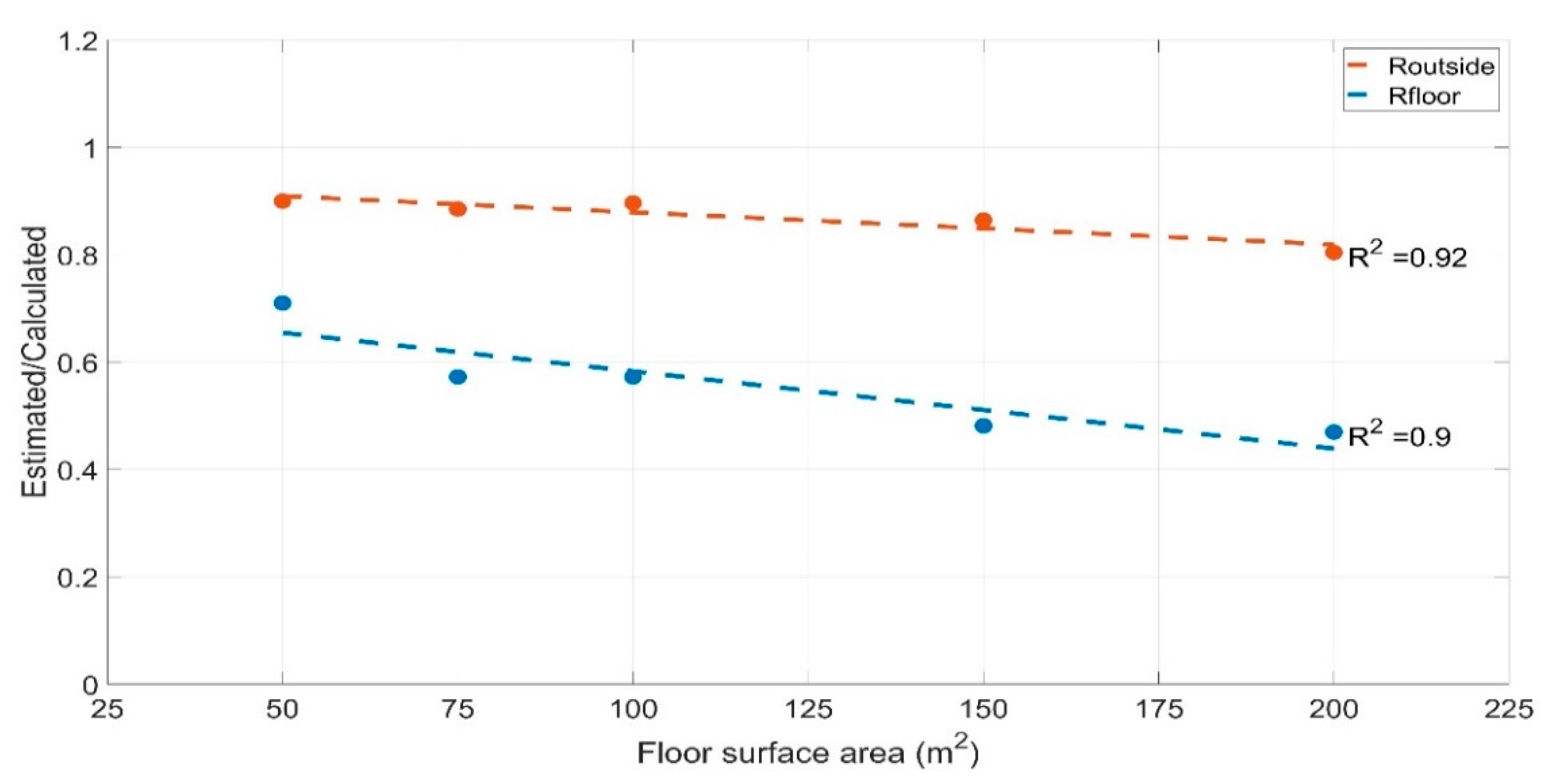
3.2. Sensitivity Analysis of Estimated Parameters in RC Model with Respect to Geometric Characteristics of Simulated Buildings in TRNSYS

In addition to the sensitivity analysis of total heat demand and peak power, it is also interesting to study the sensitivity of the estimated parameters in an RC model with respect to the specified building geometric characteristics. Using the 4R3C model for heavy- and light-structured buildings shows that for every simulated building in TRNSYS the output signal (Tin) is estimated with high accuracy. In fact, FitPercent values (Equation (10)) of more than 80% are obtained for the first 1000 h of TMY for various building’s surface areas as shown in Figure 7 and Table 8, which implies MSE values of less than 0.5 °C2. The good accuracy between the calculated indoor temperatures in TRNSYS and the RC model output signals confirms that the 4R3C model can be effectively used for various building geometries and structures.
In order to further assess how the RC model performs under real-world conditions, it is necessary to make a comparison between the estimated parameters in the RC model and their corresponding values from TRNSYS, which have been calculated according to material properties. For this purpose, the determined UA-values of the envelope (walls and roof) and the floor in TRNSYS are compared with the total thermal resistance of the envelope (Rtot = R1 + R3) and the total thermal resistance of the floor (Rfloor = R2 + R4) in the RC model. In addition, the thermal capacitances (C1, C2, and C3) in the RC model are also compared with their corresponding values in TRNSYS models for different buildings. The total thermal resistance of the envelope is equivalent to the inverse of the building UA-value. Figure 8 and Figure 9 represent the ratio between the estimated thermal resistance in the RC model and the calculated values from TRNSYS. Accordingly, using the 4R3C model confirms the accuracy of the estimated values for the total thermal resistance of the envelope for heavy- and light-structured buildings. The total thermal resistance of the envelope is estimated with an error of around 10% for heavy- and light-structured buildings for varying SA values. On the other hand, floor thermal resistances have not been estimated as accurately as the envelope thermal resistance. For both types of structure, the floor thermal resistance is underestimated from 30% up to 50%.
In addition to the thermal resistances, a close examination of Figure 10 and Figure 11 indicates that the thermal capacitances C1 and C3 are estimated in the same range of TRNSYS calculations. In the worst-case scenario, the thermal capacitance of the floor (C3) is estimated twice as large compared to that calculated by TRNSYS. On the other hand, the estimated envelope capacitances (C2) are not as accurate as the floor and internal thermal capacitances (C1 and C3). Specifically, the envelope thermal capacitances have been estimated 8 to 15 times larger than the expected values for the light-structured buildings. In the case of heavy-structured buildings, the estimated thermal capacitance of the envelope varies from 0.5 times to twice the calculated thermal capacitances by TRNSYS for various surface areas.
The difference between the estimated values of the thermal capacitance in a 4R3C model and the determined values from material properties can be attributed to a number of factors, such as:
  • Different nature of the model structures: In TRNSYS, a building is modeled with detailed information about multi-layer walls, roof, floor, windows, internal and external conditions, whereas in 4R3C model all material properties are accumulated in few parameters.
  • Different representation of model input: All input information, such as solar radiation on various walls and their distribution, are accumulated in one or two inputs that are directly inserted to a node in 4R3C model. Therefore, the state of model excitation in 4R3C model is different than TRNSYS model, where every building element is treated individually.
  • Complex nature of thermal capacitance determination in buildings: Thermal capacitances model the dynamic behavior of the building, therefore accurate estimation of thermal capacitances requires more informative dataset and experiments to excite the building under various conditions to be able to activate the thermal mass of the building in order to be captured in a data-driven model, here 4R3C model. On the contrary, average values and temperature differences and heat flows are sufficient information to estimate thermal resistances.
Low R2 values for C2 and C3 in Figure 10 confirms that the estimated values of these parameters do not show a linear behavior with respect to the specific geometric feature. It depicts further difficulties to estimate the accurate values of thermal capacitances in RC models. In fact, low value of R2 for thermal capacitances indicates that inherently greater amount of uncertainty exists in this phenomenon.
Similar graphs to Figure 8, Figure 9, Figure 10 and Figure 11 can be obtained for parameter variations of other geometric characteristics. Table 9 and Table 10 summarize the results of such an analysis for heavy- and light-structured buildings, where the minimum and maximum deviation between estimated and calculated parameters of each geometrical characteristic and their R2 error for linear regression are represented. The results show that the RC model estimates the total thermal resistance of the envelope (Renvelope = R1 + R3) with relatively good accuracy. In this case, for every simulated building, the estimated value changes from 80% up to 120% of the total thermal resistance of the envelope. The thermal resistance of the floor is also estimated with consistent deviations, which vary from 38% to 71% of the calculated value, thus it is estimated with a lower accuracy compared to the thermal resistance of the envelope. Furthermore, the internal and floor capacitances (C1 and C3) vary between 1.47 to 2.02 times their expected values. In fact, the estimated values are consistent and there are no outliers. On the other hand, the thermal capacitances of the envelope are not estimated with high accuracy since the estimated values range from 0.5 to 2.3 times and 8 to 22 times the TRNSYS values for heavy- and light-structured buildings respectively.
The outcome of this study confirms that the thermal resistance of the envelope is estimated with relatively good accuracy, changing between ±25% compared to their corresponding TRNSYS values. Furthermore, the thermal resistance of the floor is also estimated consistently but it is not estimated as accurately as the thermal resistance of the envelope. In fact, the floor thermal resistance is estimated with an accuracy of about ±50%. As shown in Figure 12, except for the thermal capacitance of the envelope C2, RC models estimate the thermal resistances and thermal capacitances (C1 and C3) with a small or reasonable deviation from the values that are calculated in TRNSYS with respect to the thermal properties of the structure.

3.3. Effects of Insulation Level on Estimated Parameters of RC Model

In order to analyze the insulation thickness effect on the accuracy of the estimated parameters of the RC model, it was assumed that the insulation thickness varies from 0 to 20 cm in the envelope and floor of a 100-2-x-0 heavy-structured building. Figure 13 shows that for different WF values the thermal resistance of the envelope is close to its TRNSYS value. The estimated UA-value varies with 20% deviation from the calculated UA-value based on material properties. In addition, the estimated UA-value of the floor also varies within a deviation of about 20%. However, for buildings with a WF value of 30%, deviations up to 50% are observed for the UA-value of the floor.
The higher WF ratios increase the impact of solar radiation distribution in a building. For instance, 30% WF ratio means a larger part of solar radiation hits the inner side of walls and floor than 5% WF ratio. Therefore, more detailed model for distribution of solar radiation would be required when the WF ratio increases. In the 4R3C model, it is assumed that the whole solar radiation through windows hits the floor and not the inner surface of walls.
Therefore, the estimated thermal capacitances of the internal mass and floor do not change significantly. However, it is noted that the thermal capacitance of the envelope for various insulation levels is estimated around half of its value compared to the calculated values from material properties in TRNSYS, as shown in Figure 14. These results highlight the difficulties to identify the thermal capacitance of the envelope with a rather good accuracy especially when more solar radiation enters a building.

4. Conclusions

This paper examines the sensitivity analysis of the total heat demand and maximum heat power, along with that of the parameters in a 4R3C model for detached buildings, with respect to relevant geometric characteristics, namely surface area, aspect ratio, windows-to-floor ratio and orientation angle. The results of this work show that although the aspect ratio, windows-to-floor ratio and orientation angle have large contributions to solar irradiation gains, the contribution of these parameters on the overall heat demand and peak power is less than 10%. Furthermore, the results confirm that the 4R3C models can estimate the indoor temperature with good accuracy compared to TRNSYS simulations regardless of the geometric characteristics of the building. It is also observed that the RC models estimate the UA-value of the envelope and the floor with good accuracy. In fact, for all simulated buildings with different geometric characteristics and structures, the UA-value of the envelope and floor are estimated with ±25% and ±50% of error respectively. On the other hand, particularly high deviations were observed on the thermal capacitance of the envelope, with values varying from 0.5 to 30 times their calculated values in TRNSYS. As a concluding remark, it is noted that the sensitivity analysis of the parameters in an RC model with respect to the geometric characteristics highlighted the strengths and weaknesses of this modelling approach, the consistency of parameters and the model accuracy to determine output signals under various conditions. Overall, it was shown that 4R3C model, can estimate thermal resistances of the structure in a close range to the values that can be obtained by material properties regardless of four different geometric characteristics.

Author Contributions

Conceptualization, A.B., V.F. and C.S.I.; methodology, A.B. and V.F.; validation, A.B. and K.N.G.; formal analysis, A.B.; investigation, A.B. and K.N.G.; data curation, A.B.; writing—original draft preparation, A.B. and K.N.G.; writing—review and editing, A.B., K.N.G. and V.F.; visualization, A.B.; supervision, V.F. and C.S.I. All authors have read and agreed to the published version of the manuscript.

Funding

This research was partially funded by the European Union’s Seventh Framework Program under grant agreement no. 621408 (RE-SIZED: Research Excellence for Solutions and Implementation of Net-Zero Energy City Districts) and Horizon 2020 Program under grant agreement no 824342 (RENAISSANCE: Renewable integration and sustainability in energy communities).

Conflicts of Interest

The authors declare no conflict of interest.

References

  1. European Commission. In Focus: Energy Efficiency in Buildings. Brussels. 17 February 2020. Available online: https://ec.europa.eu/info/sites/info/files/energy_climate_change_environment/events/documents/in_focus_energy_efficiency_in_buildings_en.pdf (accessed on 23 November 2020).
  2. Pérez-Lombard, L.; Ortiz, J.; Pout, C. A review on buildings energy consumption information. Energy Build. 2008, 40, 394–398. [Google Scholar] [CrossRef]
  3. European Parliament. Directive (EU) 2018/844 of the European Parliament and of the Council of 30 May 2018 amending Directive 2010/31/EU on the energy performance of buildings and Directive 2012/27/EU on energy efficiency. Off. J. Eur. Union 2018, 156, 75–91. [Google Scholar]
  4. European Commission. European Commission. Communication from The Commission to the European Parliament, The Council, The European Economic and Social Committee and The Committee of The Regions A Renovation Wave for Europe—Greening Our Buildings, Creating Jobs, Improving Lives. COM/2020/662 Final. Available online: https://eur-lex.europa.eu/legal-content/EN/TXT/?uri=CELEX%3A52020DC0662 (accessed on 23 November 2020).
  5. European Commission. Energy, Transport and GHG emissions: Trends to 2050, EU Reference Scenario 2016; Publications Office of the European Union: Luxembourg, 2013. [Google Scholar] [CrossRef]
  6. Iturriaga, E.; Aldasoro, U.; Terés-Zubiaga, J.; Campos-Celador, A. Optimal renovation of buildings towards the nearly Zero Energy Building standard. Energy 2018, 160, 1101–1114. [Google Scholar] [CrossRef]
  7. Good, N.; Martínez Ceseña, E.A.; Mancarella, P. Ten questions concerning smart districts. Build. Environ. 2017, 118, 362–376. [Google Scholar] [CrossRef]
  8. De Jaeger, I.; Reynders, G.; Saelens, D. Impact of spatial accuracy on district energy simulations. Energy Procedia 2017, 132, 561–566. [Google Scholar] [CrossRef]
  9. De Jaeger, I.; Reynders, G.; Ma, Y.; Saelens, D. Impact of building geometry description within district energy simulations. Energy 2018, 158, 1060–1069. [Google Scholar] [CrossRef]
  10. Loga, T.; Stein, B.; Diefenbach, N. TABULA building typologies in 20 European countries—Making energy-related features of building stocks comparable. Energy Build. 2016, 132, 4–12. [Google Scholar] [CrossRef]
  11. Schweiger, G.; Heimrath, R.; Falay, B.; O’Donovan, K.; Nageler, P.; Pertschy, R.; Engel, G.; Streicher, W.; Leusbrock, I. District energy systems: Modelling paradigms and general-purpose tools. Energy 2018, 164, 1326–1340. [Google Scholar] [CrossRef]
  12. Bagheri, A.; Feldheim, V.; Ioakimidis, C.S. On the Evolution and Application of the Thermal Network Method for Energy Assessments in Buildings. Energies 2018, 11, 890. [Google Scholar] [CrossRef] [Green Version]
  13. Bagheri, A.; Feldheim, V.; Thomas, D.; Ioakimidis, C.S. The adjacent walls effects in simplified thermal model of buildings. Energy Procedia 2017, 122, 619–624. [Google Scholar] [CrossRef]
  14. Ogunsola, O.T.; Song, L. Application of a simplified thermal network model for real-time thermal load estimation. Energy Build. 2015, 96, 309–318. [Google Scholar] [CrossRef]
  15. Harb, H.; Boyanov, N.; Hernandez, L.; Streblow, R.; Müller, D. Development and validation of grey-box models for forecasting the thermal response of occupied buildings. Energy Build. 2016, 117, 199–207. [Google Scholar] [CrossRef]
  16. Thomas, D.; Bagheri, A.; Feldheim, V.; Deblecker, O.; Ioakimidis, C.S. Energy and thermal comfort management in a smart building facilitating a microgrid optimization. In Proceedings of the IECON 2017—43rd Annual Conference of the IEEE Industrial Electronics Society, Beijing, China, 29 October–1 November 2017; pp. 3621–3626. [Google Scholar] [CrossRef]
  17. Mugnini, A.; Coccia, G.; Polonara, F.; Arteconi, A. Performance Assessment of Data-Driven and Physical-Based Models to Predict Building Energy Demand in Model Predictive Controls. Energies 2020, 13, 3125. [Google Scholar] [CrossRef]
  18. De Rosa, M.; Brennenstuhl, M.; Andrade Cabrera, C.; Eicker, U.; Finn, D.P. An Iterative Methodology for Model Complexity Reduction in Building Simulation. Energies 2019, 12, 2448. [Google Scholar] [CrossRef] [Green Version]
  19. Ahmad, T.; Chen, H.; Guo, Y.; Wang, J. A comprehensive overview on the data driven and large scale based approaches for forecasting of building energy demand: A review. Energy Build. 2018, 165, 301–320. [Google Scholar] [CrossRef]
  20. Wei, Y.; Zhang, X.; Shi, Y.; Xia, L.; Pan, S.; Wu, J.; Han, M.; Zhao, X. A review of data-driven approaches for prediction and classification of building energy consumption. Renew. Sustain. Energy Rev. 2018, 82, 1027–1047. [Google Scholar] [CrossRef]
  21. Idowu, S.; Saguna, S.; Åhlund, C.; Schelén, O. Applied machine learning: Forecasting heat load in district heating system. Energy Build. 2016, 133, 478–488. [Google Scholar] [CrossRef]
  22. TABULA WebTool. Available online: http://webtool.building-typology.eu/#bm (accessed on 7 December 2020).
  23. Kreider, J.F.; Curtiss, P.S.; Rabl, A. Heating and Cooling of Buildings: Design for Efficiency, 2nd ed.; McGraw-Hill: New York, NY, USA, 2002. [Google Scholar]
  24. Touly, Y. Study of the Impact of Changes in a building’s Geometry and Envelope on its 4R3C Model’s Components. Master Thesis, University of Mons, Mons, Belgium, 2017. [Google Scholar]
  25. Solchaga Erneta, M. Development of Thermal Network to Simulate Light Structured Buildings and Comparison with Heavy Structured Buildings. Master Thesis, University of Mons, Polytechnic University of Catalonia, Mons, Belgium, 2018. [Google Scholar]
  26. Fraisse, G.; Viardot, C.; Lafabrie, O.; Achard, G. Development of a simplified and accurate building model based on electrical analogy. Energy Build. 2002, 34, 1017–1031. [Google Scholar] [CrossRef]
  27. Ljung, L. System Identification ToolboxTM Getting Started Guide; The MathWorks, Inc.: Natick, MA, USA, 2015. [Google Scholar]
Figure 1. Visual representation of a 100-2-15-0 building: (a) 3D view; (b) floor plan (dimensions in m).
Energies 14 00657 g001
Figure 2. Visual representation of a 100-x-15-0 building with AR value equal to: (a) 0.5 or 2; (b) 1; (c) 0.25 or 4.
Energies 14 00657 g002
Figure 3. 4R3C model representing the building envelope and floor structures with two 2R1C branches.
Energies 14 00657 g003
Figure 4. Indoor and outdoor temperature, heat production, heat losses through ventilation, and solar radiation gains for a 100 m2, south-faced, heavy-structured building with WF equal to 15% simulated in TRNSYS.
Energies 14 00657 g004
Figure 5. Total heat demand and maximum power for heavy- and light-structured buildings for the first 1000 h of a TMY with respect to various geometric features (results from TRNSYS).
Energies 14 00657 g005
Figure 6. Distribution of total heat demand and maximum peak power around the average values for heavy- and light-structured buildings with respect to their surface area variations (results for 1000 h of simulation).
Energies 14 00657 g006
Figure 7. Comparison between the estimated indoor temperature of 4R3C model and TRNSYS simulation results for 100-2-15-0 building (first 1000 h of TMY).
Energies 14 00657 g007
Figure 8. Estimated/calculated ratio of resistances for different floor surface areas in x-2-15-0 light-structured buildings.
Energies 14 00657 g008
Figure 9. Estimated/calculated ratio of resistances for different floor surface areas in x-2-15-0 heavy-structured buildings.
Energies 14 00657 g009
Figure 10. Estimated/calculated ratio of capacitances for different FS values in x-2-15-0 light-structured buildings.
Energies 14 00657 g010
Figure 11. Estimated/calculated ratio of capacitances for different FS values in x-2-15-0 heavy-structured buildings.
Energies 14 00657 g011
Figure 12. Variation of total thermal resistance and capacitances compared with their values from TRNSYS: (a) light-structured building; (b) heavy-structured building.
Energies 14 00657 g012
Figure 13. Estimated/calculated ratio of thermal resistances for various WF values and insulation layer thicknesses for heavy-structured buildings: (a) building envelope; (b) floor.
Energies 14 00657 g013
Figure 14. Estimated/calculated ratio of thermal capacitances for various WF values and insulation layer thicknesses: (a) internal mass C1; (b) envelope C2; (c) floor C3.
Energies 14 00657 g014
Table 1. Material properties of roof structure consisting of 2 layers.
LayerPhysical Property [Unit]Value
Mineral woolThickness [m]0.15
Conductivity [W/m K]0.045
WoodThickness [m]0.02
Conductivity [W/mK]0.12
Capacity [J/kgK]2500
Density [kg/m3]400
Table 2. Thermal properties of floor structure consisting of 4 layers.
LayerPhysical Property [Unit]Value
TilesThickness [m]0.01
Conductivity [W/mK]1.705
Capacity [J/kgK]700
Density [kg/m3]2300
Cement mortarThickness [m]0.08
Conductivity [W/mK]1.4
Capacity [J/kgK]1000
Density [kg/m3]2000
ConcreteThickness [m]0.2
Conductivity [W/mK]2.1
Capacity [J/kgK]1000
Density [kg/m3]2400
PolyurethaneThickness [m]0.16
Conductivity [W/mK]0.03
Capacity [J/kgK]837
Density [kg/m3]35
Table 3. Thermal properties of a heavy-structured wall.
LayerPhysical Property [Unit]Value
PlasterThickness [m]0.01
Conductivity [W/mK]0.351
Capacity [J/kgK]1000
Density [kg/m3]1500
Concrete blocsThickness [m]0.2
Conductivity [W/mK]1.053
Capacity [J/kgK]650
Density [kg/m3]1300
Polystyrene expandedThickness [m]0.16
Conductivity [W/mK]0.039
Capacity [J/kgK]1380
Density [kg/m3]25
Exterior coat (clay)Thickness [m]0.01
Conductivity [W/mK]1.153
Capacity [J/kgK]1000
Density [kg/m3]1700
Table 4. Thermal properties of a light-structured wall.
LayerPhysical Property [Unit]Value
PlasterboardThickness [m]0.01
Conductivity [W/mK]0.331
Capacity [J/kgK]801
Density [kg/m3]790
CompositeThickness [m]0.14
Conductivity [W/mK]0.671
Capacity [J/kgK]876
Density [kg/m3]60.8
Glass woolThickness [m]0.09
Conductivity [W/mK]0.041
Capacity [J/kgK]840
Density [kg/m3]12
Table 5. Physical characteristics of insulation material.
Material PropertyUnitValue
Conductivity W/mK0.03
Capacity J/kgK837
Density kg/m335
Table 6. Compactness of buildings with different SA values and AR equal to 2.
SA (m²)Side Walls Surface (m2)Front/Back Walls Surface (m2)Volume (m3)Compactness
5015.0030.001500.79
7518.3736.742250.86
10021.2142.423000.92
15025.9851.964500.99
20030.0060.006001.03
Table 7. Surface of windows in each wall for 100-2-x-0 buildings.
WFWindows Surface on the Front Wall (m2)Windows Surface on the Side Wall (m2)
5%2.501.25
10%5.002.50
15%7.503.75
20%10.005.00
30%15.007.50
Table 8. FitPercent calculations for heavy- and light-structured buildings with various SA values (x-2-15-0). (Evaluated for the first 1000 h of TMY).
SA (m²)FitPercent for Light-Structured BuildingFitPercent for Heavy-Structured Building
5083.7685.53
7584.3986.01
10083.1586.23
15082.0086.41
20083.1786.82
Table 9. Linear regression results of estimated/calculated parameters for heavy-structured buildings.
x-2-15-0
SA
100-2-x-0
WF
100-x-15-0
AR
100-2-15-x
OA
minmaxR2minmaxR2minmaxR2minmaxR2
Renvelope0.800.900.920.800.970.990.870.930.990.870.900.75
Rfloor0.470.710.900.380.600.960.550.570.950.520.620.62
C10.960.990.840.950.990.910.960.970.690.960.970.05
C20.452.040.420.384.410.840.554.141.000.672.280.12
C31.902.020.971.952.030.111.912.031.001.941.950.57
Table 10. Linear regression of estimated/calculated parameters for light-structured buildings.
x-2-15-0
SA
100-2-x-0
WF
100-x-15-0
AR
100-2-15-x
OA
minmaxR2minmaxR2minmaxR2minmaxR2
Renvelope1.021.120.610.951.200.971.041.091.001.051.050.79
Rfloor0.460.680.650.430.620.740.450.530.990.490.620.98
C10.951.300.981.131.180.021.131.241.001.121.160.97
C28.4014.540.917.4422.710.537.7111.060.979.2122.060.99
C31.261.600.661.411.580.381.471.530.981.391.500.98
Publisher’s Note: MDPI stays neutral with regard to jurisdictional claims in published maps and institutional affiliations.

